runoff.pdf

1
RUNOFF CALCULATIONS
1.
To estimate the magnitude of a flood peak the following alternative
methods are available:
2.
Unit-hydrograph technique
3.
Empirical method
Semi-Empirical method (such rational method).
1.
There many empirical or Semi-Empirical formulae used to estimate the
runoff discharge from catchment area. These formulae can be classify into
three categories;
Formulae consider the area only into calculation, like Dickens, Ryves,
Ingles and others. The formulae take forms as Q=CAn
2.
; n exponent is
almost ˂1.
3.
Formulae consider Area and some other factors such as Craig , Lillie
and Rhinds (Taking velocity , and may be intensity, depth or max,
depth of rainfall).
Formulae consider the recurrence interval ,like Fullers , Hortons ,
Pettis and other.
The use of a particular method depends upon (i) the desired objective, (ii)
the available data, and (iii) the importance of the project.
Above all , two methods depend on semi-empirical bases are preferable
for storm design ,and have a wide use by the designer. The Rational
method and the SCS-CN method . Further the Rational formula is only
applicable to small-size (< 50 km2
) catchments and the unit-hydrograph
method is normally restricted to moderate-size catchments with areas less
than 5000 km2
RATIONAL METHOD
Consider a rainfall of uniform intensity and duration occurring over a
basin in a time taken for a drop of water from the farthest part of the
catchment to reach the outlet that called tc = time of concentration, it is
obvious that if the rainfall continues beyond tc, the runoff will be constant
and at the peak value. The peak value o f the runoff is given by;

2
𝑄𝑄𝑄𝑄 = 𝐶𝐶 𝑖𝑖 𝐴𝐴 ; 𝑓𝑓𝑓𝑓𝑓𝑓 𝑡𝑡 > 𝑡𝑡𝑡𝑡 − − − − − − − − − (1)
Where,
C = coefficient of runoff = (runoff/rainfall), A = area of the catchment
and i = intensity of rainfall.
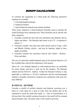
To quantify peak runoff discharge 𝑄𝑄𝑄𝑄, is examined in Figure 1.
The simulation of above equation is quoted from the following;
Fig.(1) Relationship of rainfall intensity to runoff for an impervious
drainage basin according to the Rational Method.
The total volume of runoff equals the area under the graph of runoff versus
time. Thus, volume is computed in (m3
) if 𝑡𝑡𝑡𝑡 in second 𝑄𝑄𝑄𝑄 in (m3
But remember that because the drainage basin is assumed hypothetically
completely impervious, total runoff equals total rainfall. Total rainfall is
computed simply as the depth of rainfall (m) times the area (m
/s) as;
𝑉𝑉𝑉𝑉𝑉𝑉𝑉𝑉𝑉𝑉𝑉𝑉 =
1
2
(2)(𝑡𝑡𝑡𝑡)(𝑄𝑄𝑄𝑄)
= 𝑡𝑡𝑡𝑡 𝑄𝑄𝑄𝑄
2
) over
which the rainfall occurred. Depth of rainfall is the rainfall intensity
(cm/hr) converted to (m/s) times the duration used in seconds. Thus,
Depth =
𝑖𝑖
100(3600)
(tc)
=
𝑖𝑖
3.6 × 105
𝑡𝑡𝑡𝑡
and rainfall volume is
𝑉𝑉𝑉𝑉𝑉𝑉𝑉𝑉𝑉𝑉𝑉𝑉 = 𝐷𝐷𝐷𝐷𝐷𝐷𝐷𝐷ℎ × 𝐴𝐴𝐴𝐴𝐴𝐴𝐴𝐴(km2
)

3
𝑉𝑉𝑉𝑉𝑉𝑉𝑉𝑉𝑉𝑉𝑉𝑉 =
𝑖𝑖
3.6 × 105
× 𝑡𝑡𝑡𝑡 × 𝐴𝐴 × 106
Finally, equating the volumes gives;
𝑡𝑡𝑡𝑡 𝑄𝑄𝑄𝑄 =
𝑖𝑖
3.6 × 105
× 𝑡𝑡𝑡𝑡 × 𝐴𝐴 × 106
or;
𝑄𝑄𝑄𝑄 = 2.78 𝑖𝑖 𝐴𝐴 , (𝑨𝑨 𝑖𝑖𝑖𝑖 𝑘𝑘𝑘𝑘2
𝑎𝑎𝑎𝑎𝑎𝑎 𝒊𝒊 𝑖𝑖𝑖𝑖 (𝑐𝑐𝑐𝑐/ℎ𝑟𝑟)
This is the basic equation of the rational method for drainage basin that
assumed completely impervious
𝑄𝑄𝑄𝑄 = 2.78 𝐶𝐶 (𝑖𝑖𝑡𝑡𝑡𝑡.𝑝𝑝 )𝐴𝐴 − − − − − − − − − − − − − − − −(2)
. Using the commonly used units, Eq. (1)
is re-written for field application as;
Where
𝑄𝑄𝑄𝑄 = peak discharge (m3
/s)
𝑖𝑖𝑡𝑡𝑡𝑡.𝑝𝑝 = the mean intensity of precipitation (cm/ hr) for a duration equal to
tc and an exceedence probability P.
C = Coefficient of runoff
𝐴𝐴 = drainage area in km2
The use of this method to compute 𝑄𝑄𝑄𝑄 requires three parameters: 𝑡𝑡𝑡𝑡, 𝑖𝑖𝑡𝑡𝑡𝑡.𝑝𝑝 ,
and C .
Time of Concentration ( tc)
There are a number of empirical equations available for the estimation of
the time of concentration. One of these are described below:
Kirpich Equation (1940) This is the popularly used formula relating the
time of concentration of the length of travel and slope of the catchment
𝑡𝑡𝑡𝑡 in minutes.
as;
𝑡𝑡𝑡𝑡 =
0.01947𝐿𝐿0.77
𝑆𝑆0.385
− − − − − − − − − − − − − − − −(3)
Where;
L = maximum length of travel of water (m),
S = slope of the catchment = ΔH/L in which
ΔH =difference in elevation between the most remote point on the
catchment and the outlet.

4
Rainfall Intensity (𝑖𝑖𝑡𝑡𝑡𝑡.𝑝𝑝 )
The rainfall intensity corresponding to a duration tc and the desired
probability of exceedence P, ( i.e. return period T=1/P ) is found from the
rainfall-frequency-duration relationship for the given catchment area;
𝑖𝑖𝑡𝑡𝑡𝑡.𝑝𝑝 =
𝐾𝐾𝑇𝑇𝑥𝑥
(𝑡𝑡𝑡𝑡 + 𝑎𝑎)𝑛𝑛
in which the coefficients K. a, x and n are specific to a given area.
Runoff Coefficient (C)
The coefficient C represents the integrated effect of the catchment losses
and hence depends upon the nature of the surface, surface slope and
rainfall intensity. The effect of rainfall intensity is not considered in the
available tables of values of C. Some typical values of C are indicated in
Table (1) and Table (2). Equation (2) assumes a homogeneous catchment
surface. If however, the catchment is non-homogeneous but can be divided
into distinct sub areas each having a different runoff coefficient, then the
runoff from each sub area is calculated separately and merged in proper
time sequence. Sometimes, a non-homogeneous catchment may have
component sub areas distributed in such a complex manner that distinct
sub zones cannot be separated. In such cases a weighted equivalent runoff
coefficient 𝐶𝐶𝐶𝐶 as below is used.
𝐶𝐶𝐶𝐶 =
∑ 𝐶𝐶𝑖𝑖𝐴𝐴𝑖𝑖
𝑁𝑁
1
𝐴𝐴
− − − − − − − − − − − − − − − − − (4)
where 𝐴𝐴𝑖𝑖= the areal extent of the sub area i having a runoff coefficient Ci
and N = number of sub areas in the catchment.
The rational formula is found to be suitable for peak-flow prediction in
small catchments up to 50 km2
in area. It finds considerable application in
urban drainage designs and in the design of small culverts and bridges.
It should be noted that the word rational is rather a misnomer as the
method involves the determination of parameters tc and C in a
subjective manner.

5
Table (1) Value of the Coefficient C in Eq. (2)
Table (2) Values of C in Rational Formula for Watersheds with
Agricultural an d Forest Land Covers

6
Example (1)
An urban catchment has an area o f 85 ha. The slope of the catchment
is 0.006 and the maximum length o f travel o f water is 950 m. The
maximum depth of rainfall with a 25-year return period is as below:
If a culvert for drainage at the outlet o f this area is to be designed for a
return period of 25 years, estimate the required peak-flow rate, by
assuming the runoff coefficient as 0.3.
Solution:
The time of concentration is obtained by the Kirpich formula as;
𝑡𝑡𝑡𝑡 =
0.01947𝐿𝐿0.77
𝑆𝑆0.385
=
0.01947(950)0.77
(0.006)0.385
= 27.4 𝑚𝑚𝑚𝑚𝑚𝑚𝑚𝑚𝑚𝑚𝑚𝑚𝑚𝑚
By interpolation,
Maximum depth of rainfall for 27.4 min duration:
=
(5 0 −4 0 )
30−20
=
(𝑥𝑥 −4 0 )
27.4−20
𝑥𝑥 =
(5 0 −4 0 )
30−20
× 7.4 + 40 = 47.4 𝑚𝑚𝑚𝑚
Average intensity = 𝑖𝑖𝑡𝑡𝑡𝑡.𝑝𝑝 =
𝑑𝑑𝑑𝑑𝑑𝑑𝑑𝑑 ℎ
𝑑𝑑𝑑𝑑𝑑𝑑𝑑𝑑𝑑𝑑𝑑𝑑𝑑𝑑𝑑𝑑
=
47.4/10
27.4/60
= 10.38 𝑐𝑐𝑐𝑐/ℎ𝑟𝑟
Recalling Eq. (2) :
𝑄𝑄𝑄𝑄 = 2.78 (0.3)(10.38)(0.85) = 7.35 𝑚𝑚3
/𝑠𝑠
Example (2)
If in the urban area o f Example (1), the land use o f the area and the
corresponding runoff coefficients are as given below, calculate the
equivalent runoff coefficient.
Solution
The equivalent runoff coefficient 𝐶𝐶𝐶𝐶 =
∑ 𝐶𝐶𝑖𝑖𝐴𝐴𝑖𝑖
𝑁𝑁
1
𝐴𝐴
𝐶𝐶𝐶𝐶 =
0.7 × 8 + 0.1 × 17 + 0.3 × 50 + 0.8 × 10
8 + 17 + 50 + 10
=
30.3
85
= 0.36
Duration (min) 5 10 20 30 40 60
Max. Depth of rainfall (mm) 17 26 40 50 57 62

7
Example (3)
An engineer is required to design a drainage system for an airport of area
2.5 km2
𝑖𝑖 =
𝑇𝑇
(𝑡𝑡+10)0.38
; where i=rainfall intensity in cm/hr, and t=duration in
minutes. T=return period in year.
for 35 year return period .if the equation of rainfall intensity is;
If the concentration time for the area is estimated as 50 minutes ,for what
discharge the system must design?
Solution
𝑖𝑖 =
𝑇𝑇
(𝑡𝑡 + 10)0.38
=
35
(50 + 10)0.38
𝑄𝑄𝑄𝑄 = 2.78 (1)(7.385)(2.5) = 51.32 𝑚𝑚3
/𝑠𝑠
A watershed of 500 ha has the land use/cover and corresponding runoff
coefficient as given below:
HW1:
The maximum length o f travel o f water in the watershed is about 3000 m
and the elevation difference between the highest and outlet points o f the
watershed is 25 m. The maximum intensity duration frequency relationship
o f the watershed is given by;
𝑖𝑖 =
6.311 𝑇𝑇0.1523
(𝐷𝐷 + 0.5)0.945
Where;
i = intensity in cm/h, T = Return period in years and D = duration of the
rainfall in hours.

8
Estimate the (i) 25 year peak runoff from the watershed and (ii) the 25
year peak runoff if the forest cover has decreased to 50 ha and the
cultivated land has encroached upon the pasture and forset lands to have
a total coverage of 450 ha.
Solution of HW
Case 1: Equivalent runoff coefficient:
Ce = [(0.10 × 250) + (0.11 × 50) + (0.30 × 200)] /500=0.181
time of concentration 𝑡𝑡𝑡𝑡 =
0.01947(3000)0.77
(
25
3000
)0.385
= 58.51 min=0.975 hr
Calculation of 𝑖𝑖𝑡𝑡𝑡𝑡.𝑝𝑝 :
Here D = tc = 0.975 hr. T= 25 years. Hence
𝑖𝑖 =
6.311 (25)0.1523
(0.975 + 0.5)0.945
Peak Flow by Eq. (2), Qp = 2.78Ce i A
=2.78× 0.181 × 7.123 × (500/100) ,
= 17.92 m3
/s
Case 2: Here Equivalent C = Ce = [(0.10×50)+ (0.30×450)]/500=0.28
i = 7.123 cm/hr and A = 500 ha = 5 km
Qp = 2.78Ce i A = 2.78× 0.28 × 7.123 × (500/100) = 27.72 m
2
3
/s

9
SCS-CN method, developed by Soil Conservation Services (SCS) of USA
in 1969, is a simple, predictable, and stable conceptual method for
estimation of direct runoff depth based on storm rainfall depth. It relies on
only one parameter, CN. The details of the method are described in this
section.
SCS-CN Method to estimate Runoff
Basic Theory
The SCS-CN method is based on the water balance equation of the rainfall
in a known interval of time Δt, referring to Fig.(2) and from the continuity
principle it can be expressed as;
𝑃𝑃 = 𝐼𝐼𝐼𝐼 + 𝐹𝐹𝐹𝐹 + 𝑃𝑃𝑃𝑃 − − − − − − − − − − − − − − − −(5)
where
P = total precipitation,
Ia= initial abstraction,
Fa = Cumulative infiltration excluding Ia and,
Pe = direct surface runoff (all in units of volume occurring in time Δt).
Two other concepts as below are also used with Eq. (5).
(i) The first concept is that the ratio of actual amount of direct runoff ,Pe
to maximum potential runoff (= P- Ia) is equal to the ratio of actual
infiltration (Fa ) to the potential maximum retention (or infiltration), S.
This proportionality concept can be schematically shown as in Fig.
𝑃𝑃𝑃𝑃
𝑃𝑃−𝐼𝐼𝐼𝐼
=
𝐹𝐹𝐹𝐹
𝑆𝑆
− − − − − − − − − (6)
(ii) The second concept is that the amount of
initial abstraction (Ia) is some fraction
of the potential maximum retention (.S).
Thus ;
𝐼𝐼𝐼𝐼 = 𝜆𝜆 𝑆𝑆 − − − − − − − − − − − − − (7)

10
Combining Eqs. (6) and (7), and using (5)
𝑃𝑃𝑃𝑃 =
( 𝑃𝑃 – 𝐼𝐼𝐼𝐼)2
𝑃𝑃 – 𝐼𝐼𝐼𝐼 + 𝑆𝑆
=
( 𝑃𝑃 – 𝜆𝜆 𝑆𝑆)2
𝑃𝑃 + (1 − 𝜆𝜆 )𝑆𝑆
; for 𝑃𝑃 > 𝜆𝜆𝜆𝜆 − − − − − −(8)
𝑃𝑃𝑃𝑃 = 0 𝑓𝑓𝑓𝑓𝑓𝑓 𝑃𝑃 ≤ 𝜆𝜆𝜆𝜆
𝐼𝐼𝐼𝐼 𝑃𝑃 < 𝐼𝐼𝐼𝐼 𝑡𝑡ℎ𝑒𝑒𝑒𝑒 𝑃𝑃𝑃𝑃 = 0 𝑤𝑤ℎ𝑖𝑖𝑖𝑖𝑖𝑖 𝑖𝑖𝑖𝑖 𝑃𝑃 > 𝐼𝐼𝐼𝐼 𝑡𝑡ℎ𝑒𝑒𝑒𝑒 𝑃𝑃𝑃𝑃 𝑐𝑐𝑐𝑐𝑐𝑐 𝑏𝑏𝑏𝑏 𝑐𝑐𝑐𝑐𝑐𝑐𝑐𝑐𝑐𝑐𝑐𝑐𝑐𝑐𝑐𝑐𝑐𝑐𝑐𝑐 .
Value of λ
On the basis of extensive measurements in small size catchments SCS
(1985) adopted λ = 0.2 as a standard value, then Eq. (8) becomes;
𝑃𝑃𝑃𝑃 =
( 𝑃𝑃 – 0.2 𝑆𝑆)2
𝑃𝑃 + 0.8𝑆𝑆
; for 𝑃𝑃 > 0.2𝑆𝑆
For operation purposes a time interval Δt = 1 day is adopted. Thus P= daily
rainfall and Pe= daily runoff from the catchment.
Curve Number (CN)
The parameter S representing the potential maximum retention depends
upon :
1. The soil-vegetation-land use complex of the catchment.
2. the antecedent soil moisture condition in the catchment just prior to the
commencement of the rainfall event.
For convenience in practical application the Soil Conservation Services
(SCS) has expressed S (mm) in terms of a dimensionless parameter CN
(the Curve number) as;
𝑆𝑆 =
25400
𝐶𝐶𝐶𝐶
− 254 = 254 �
100
𝐶𝐶𝐶𝐶
− 1� − − − − − − − − − − − − (9)
The constant 254 is used to express S in mmThe curve number CN is now
related to S as;
𝐶𝐶𝐶𝐶 =
25400
𝑆𝑆 + 254
and has a range of 0 < CN< 100.
CN = 100 represents zero potential retention (i.e. impervious catchment)
CN = 0 represents an infinitely abstracting catchment with S =∞.
Curve number CN depends upon:
a) Soil type , b) Antecedent moisture condition , c) Land use/cover

11
a)Soils:
In the determination of CN, the hydrological soil classification is adopted.
Here, soils are classified into four classes A, B, C and D based upon the
infiltration and other characteristics. The important soil characteristics that
influence hydrological classification of soils are effective depth of soil,
average clay content, infiltration characteristics and permeability.
• Group-A: ( Low Runoff Potential ): Soils having high infiltration rates
even when thoroughly wetted. These soils have high rate of water
transmission. [Example: Deep sand, Deep loess and Aggregated silt].
• Group-B: (Moderately Low runoff Potential): Soils having moderate
infiltration rates when thoroughly wetted. These soils have moderate rate
of water transmission. [Example: Shallow loess, Sandy loam, Red loamy
soil, Red sandy loam and Red sandy soil ].
• Group-C: ( Moderately High Runoff Potential): Soils having low
infiltration rates when thoroughly wetted. These soils have moderate rate
of water transmission. [Example: Clayey loam, Shallow sandy loam, Soils
usually high in clay, Mixed red and black soils].
• Group-D: (High Runoff Potential): Soils having very low infiltration rates
when thoroughly wetted and consisting chiefly of clay soils with a high
swelling potential, soils with a permanent high-water table, soils with a
clay layer near the surface.[Example: Heavy plastic clays, certain saline
soils and deep black soils].
b)Antecedent Moisture Condition
(AMC) refers to the moisture content present in the soil at the beginning of
the rainfall-runoff event under consideration. It is well known that initial
abstraction and infiltration are governed by AMC. For practical application
three levels of AMC are recognized by SCS as follows:
AMC-I: Soils are dry but not to wilting point. Satisfactory cultivation has
taken place.
AMC-II: Average conditions
AMC-III: Sufficient rainfall has occurred within the immediate past 5 days.
Saturated soil conditions prevail.

12
T able (3) Antecedent Moisture Conditions (AMC) for Determining the
Value of CN.
c) Land Use/cover
The variation of CN under AMC-II, called CNII, for various land use
conditions commonly found in practice are shown in Table (4) (a, b and c).
Table (4-a) Runoff Curve Numbers ( CNII ) for Hydrologic Soil Cover
Complexes ( Under AMC-II Conditions)
Note: Sugarcane has a separate supplementary Table of CNI values (Table
4-b) The conversion of CNII to other two AMC conditions can be made
through the use of following correlation equations.
For AMC-I: 𝐶𝐶𝐶𝐶𝐼𝐼 =
𝐶𝐶𝐶𝐶𝐼𝐼𝐼𝐼
12.281 − 0.01281𝐶𝐶𝐶𝐶𝐼𝐼𝐼𝐼
− − − − − (11)

13
Table (4-b) CNII Values for Sugarcane
Table (4-c) CNII Values for Suburban and Urban Land Uses
For AMC-III: 𝐶𝐶𝐶𝐶𝐼𝐼𝐼𝐼𝐼𝐼 =
𝐶𝐶𝐶𝐶𝐼𝐼𝐼𝐼
0.427+ 0.00573𝐶𝐶𝐶𝐶𝐼𝐼𝐼𝐼
− − − − − (12)
The equations (11) and (12) are applicable in the CNII, range of 55 to 95
which covers most of the practical range.
λ=0.1 valid for Black soils under AMC of Type II and III.
Notes about λ
λ=0.3 valid for Black soils under AMC of Type I and for all other
soils(excluding Black soil) having AMC of types I, II and III.
Example (4)
In a 350 ha watershed the CN value was assessed as 70 for AMC-III.
a) Estimate the value o f direct runoff volume for the following 4 days of rainfall.
The AMC on July 1st was of category III. Use standard SCS-CN equations.
b) What would be the runoff volume if the CNIII value were 80?

14
a) Given CNIII = 70 S = (25400/70) - 254 = 108.6mm
𝑃𝑃𝑃𝑃 =
( 𝑃𝑃 – 0.2 𝑆𝑆)2
𝑃𝑃𝑃𝑃 =
[𝑃𝑃 − (0.2 )108.6]2
𝑃𝑃 + 0.8(108.6)
=
[𝑃𝑃 – 21.78]2
𝑃𝑃 + 87.09
; 𝑓𝑓𝑓𝑓𝑓𝑓 𝑃𝑃 > 21.78 mm
Solution
Total runoff volume over the catchment Vr = 350 × 104
= 22,365 m
× 6.39/1000
b) Given CNIII = 80 S = (25400/80) - 254 = 63.5 mm
𝑃𝑃𝑃𝑃 =
( 𝑃𝑃 – 0.2 𝑆𝑆)2
𝑃𝑃𝑃𝑃 =
[𝑃𝑃 − (0.2 )63.5]2
𝑃𝑃 + 0.8(63.5)
=
[𝑃𝑃 – 12.70]2
𝑃𝑃 + 50.80
; 𝑓𝑓𝑓𝑓𝑓𝑓 𝑃𝑃 > 12.70 mm
3
= 65,310m
× 18.66/1000
Example (5)
3
A small watershed is 250 ha in size has group C soil. The land cover can be
classified as 30% open forest and 70% poor quality pasture. Assuming
AMC at average condition and the soil to be black soil, estimate the direct
runoff volume due to a rainfall o f 75 mm in one day.

15
AMC = II . Hence CN = CNII . Soil = Black soil. Referring to Table
Solution
(4-a) for C-group soil;
Average CN = 7820/100 = 78.2 S = (25400/78.2) - 254 = 70.81mm
The relevant runoff equation for Black soil and AMC-II is(λ=0.1) ;
𝑃𝑃𝑃𝑃 =
( 𝑃𝑃 – 0.1 𝑆𝑆)2
𝑃𝑃𝑃𝑃 =
[𝑃𝑃 − (0.1 )70.81]2
𝑃𝑃 + 0.9(70.81)
= 33.25 ; 𝑓𝑓𝑓𝑓𝑓𝑓 𝑃𝑃 > 7.08 mm
= 83,125 m
× 33.25/(1000)
3
Example (5)
The land use and soil characteristics of a 5000 ha watershed are as
follows:
Soil: Not a black soil.
Hydrologic soil classification: 60% is Group B and 40% is Group C
Land Use:
Hard surface areas = 10%
Waste Land = 5%
Orchard (without understory cover) = 30%
Cultivated (Terraced), poor condition = 55%
Antecedent rain: The total rainfall in past five days was 30 mm. The season
is dormant season.
(a) Compute the runoff volume from a 125 mm rainfall in a day on the
watershed
(b) What would have been the runoff if the rainfall in the previous 5 days
was 10 mm?
(c) If the entire area is urbanized with 60% residential area (65% average
impervious area), 10% of paved streets and 30% commercial and
business area (85% impervious),
estimate the runoff volume under AMC-II condition for one day rainfall
of 125 mm.

16
Solution
a) Calculation of weighted CN; From Table (3) AMC = Type III. Using
Table (4-a) weighted CNII is calculated as below ;
Weighted 𝐶𝐶𝐶𝐶 =
(4089+ 3056)
100
= 71.45
100
By Eq. (12) ; 𝐶𝐶𝐶𝐶𝐼𝐼𝐼𝐼𝐼𝐼 =
71.45
0.427+ 0.00573(71.45)
= 85.42
Since the soil is not a black soil, λ=0.3 is used to compute the surface
runoff.
𝑃𝑃𝑃𝑃 =
( 𝑃𝑃 – 0.3 𝑆𝑆)2
𝑆𝑆 = 25400/𝐶𝐶𝐶𝐶 − 254 = (25400/85.42) − 254 = 43.35 mm
𝑃𝑃𝑃𝑃 =
( 125 – (0.3) 43.35)2
125 + 0.7(43.35)
= 80.74 𝑚𝑚𝑚𝑚
= 4,037,000 m
× 80.74/(1000)
3
= 4.037 Mm
b) Here AMC = Type I , and use Eq.( 11) to get CNI;
𝐶𝐶𝐶𝐶𝐼𝐼 =
71.45
2.281 − 0.01281(71.45)
= 52.32
𝑆𝑆 = 25400/52.32 − 254 = 231.47
𝑃𝑃𝑃𝑃 =
( 125 – (0.3) 231.47)2
125 + 0.7(231.475)
= 10.75 𝑚𝑚𝑚𝑚
3
Total runoff volume over the catchment Vr = 5000 ×104
= 537500 m
× 10.75/(1000)
3

17
For Hydrological soil Group (HSG) type B
for Pasture of Good cover(Under AMC-II
Conditions), calculate the runoff volume by
SCS-CN method.
HW2
Solution of HW
From Table (4-a): CNII =61
𝑆𝑆 =
25400
𝐶𝐶𝐶𝐶
− 254 = �
25400
61
� − 254 = 162.4𝑚𝑚𝑚𝑚
𝑃𝑃𝑃𝑃 =
( 𝑃𝑃 – 𝜆𝜆𝜆𝜆)2
𝑃𝑃 + 𝜆𝜆 𝑆𝑆
; for 𝑃𝑃 > 𝜆𝜆𝜆𝜆
Use λ -standard (λ =0.2):
𝑃𝑃𝑃𝑃 =
( 110 – (0.2)162.4)2
110 + 0.8(162.4)
=
( 110 – 32.48)2
110 + 129.92
= 25.05 𝑚𝑚𝑚𝑚
Total runoff volume over the catchment Vr = 6000 ×5000 × 25.05/(1000)
= 751,500 m3

runoff.pdf

Recommended

Recommended

More Related Content

What's hot

What's hot (20)

Similar to runoff.pdf

Similar to runoff.pdf (20)

Recently uploaded

Recently uploaded (20)

runoff.pdf