A document on design of experiments (DOE) is summarized as follows:
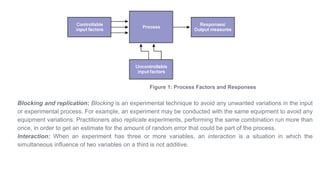
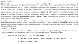
DOE is a systematic method to determine the relationship between factors affecting a process and its output. Experiments involve the systematic collection of data with a focus on the design itself rather than results. Factors that can be modified are called controllable inputs or x-factors, while uncontrollable inputs cannot be changed. Hypothesis testing uses statistical methods to determine significant factors. Blocking and replication are used to reduce unwanted variations and estimate random error. Interactions occur when the simultaneous influence of two variables on a third is not additive. Well-designed experiments can optimize processes and solve problems.