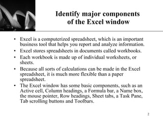
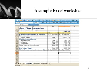
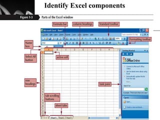
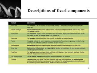
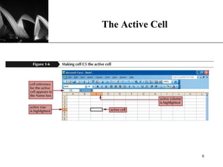
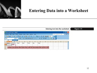
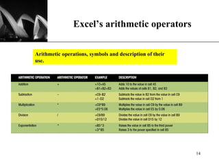
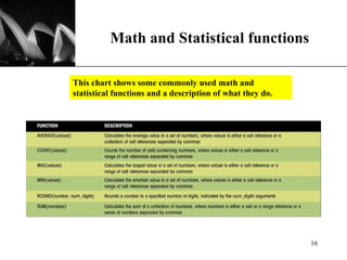
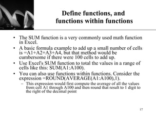
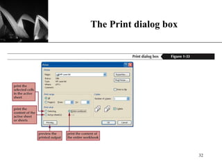
Microsoft Excel   By: Ankita jain   Varnit agarwal
Identify major components  of the Excel window Excel is a computerized spreadsheet, which is an important business tool that helps you report and analyze information.  Excel stores spreadsheets in documents called workbooks.  Each workbook is made up of individual worksheets, or sheets.  Because all sorts of calculations can be made in the Excel spreadsheet, it is much more flexible than a paper spreadsheet.  The Excel window has some basic components, such as an Active cell, Column headings, a Formula bar, a Name box, the mouse pointer, Row headings, Sheet tabs, a Task Pane, Tab scrolling buttons and Toolbars.
A sample Excel worksheet
Identify Excel components New Perspectives  on Microsoft Office Excel 2003, Second Edition- Tutorial 1
Descriptions of Excel components
Navigate within worksheets To navigate within a workbook, you use the arrow keys, PageUp, PageDown, or the Ctrl key in combination with the arrow keys to make larger movements.  The most direct means of navigation is with your mouse.  Scroll bars are provided and work as they do in all Windows applications.
Navigate between worksheets To move to other Worksheets, you can:  Click their tab with the mouse Use the Ctrl key with the Page Up and Page Down keys to move sequentially up or down through the worksheets If you are familiar with Microsoft Access, you will find the tab scrolling buttons for moving between worksheets to be similar to record browsing on an Access form or datasheet.
Navigation keystrokes
The Active Cell
Developing a Worksheet Determine the worksheet’s purpose. Enter the data and formulas. Test the worksheet and make any necessary edits / corrections. Document the worksheet and improve appearance. Save and print the complete worksheet.
Entering Data into a Worksheet To enter data, first make the cell in which you want to enter the data active by clicking it. Enter the data (text, formulas, dates, etc.) into the active cell. Use the Alt+Enter key combination to enter text on multiple lines within the same cell. Use TAB key, arrow keys, or ENTER key to navigate among the cells.
Entering Data into a Worksheet
Entering Formulas A formula is a mathematical expression that calculates a value. In Excel, formulas always begin with an equal sign (=). A formula can consist of one or more arithmetic operators. The order of precedence is a set of predefined rules that Excel follows to calculate a formula.
Excel’s arithmetic operators Arithmetic operations, symbols and description of their use.
Work with the Insert Function button Excel supplies more than 350 functions organized into 10 categories: Database, Date and Time, Engineering, Financial, Information, Logical, Lookup, Math, Text and Data, and Statistical functions You can use the Insert Function button on the Formula bar to select from a list of functions.  A series of dialog boxes will assist you in filling in the arguments of the function and this process also enforces the use of proper syntax.
Math and Statistical functions This chart shows some commonly used math and statistical functions and a description of what they do.
Define functions, and  functions within functions The SUM function is a very commonly used math function in Excel.  A basic formula example to add up a small number of cells is =A1+A2+A3+A4, but that method would be cumbersome if there were 100 cells to add up.  Use Excel's SUM function to total the values in a range of cells like this: SUM(A1:A100). You can also use functions within functions. Consider the expression =ROUND(AVERAGE(A1:A100),1). This expression would first compute the average of all the values from cell A1 through A100 and then round that result to 1 digit to the right of the decimal point
Examine the Insert Function  dialog box This dialog box appears when you click the Insert Function button. It can assist you in defining your function.
Resize worksheet rows and columns There are a number of methods for altering row height and column width using the mouse or menus:  Click the dividing line on the column or row, and drag the dividing line to change the width of the column or height of the row  Double-click the border of a column heading, and the column will increase in width to match the length of the longest entry in the column Widths are expressed either in terms of the number of characters or the number of screen pixels.
Resize a column
Create column and pie  charts in Excel Charts, or graphs, provide visual representations of the workbook data.  A chart may be embedded in an existing worksheet, or can be created on a separate chart sheet, with its own tab in the workbook. You can use Excel’s Chart Wizard to quickly and easily create charts. The Chart Wizard is a series of dialog boxes that prompt you for information about the chart you want to generate
Create a chart using the Chart Wizard To create a chart with the Chart Wizard: Select the data you want to chart, which will be your data source Click the Chart Wizard button on the standard toolbar  In the first step of the chart wizard, select the chart type and sub-type In the second step of the Chart Wizard, make any additions or modifications to the chart's data source  In the third step, make any modifications to the chart's appearance In the fourth and final step, specify the location for the chart, then click the OK button
Chart Wizard dialog box 1 Choose a chart type and view examples of that type in dialog box 1. Choose which type of chart you want in this pane. Select a sub-type of that chart in this pane. Click and hold this button down to see a preview of your chart.
Choosing a data series You can alter the data source during step 2 of the Chart Wizard and also choose whether to organize the data source by rows or by columns.  The data source is organized into a collection of data series.  A data series consists of data values, which are plotted on the chart's vertical, or Y-axis  The data series’ category values, or X values, are on the horizontal axis, called the X-axis A chart can have several data series all plotted against a common set of category values.
Chart Wizard dialog box 2 During the second step of the Chart Wizard, you specify the data to be displayed in the chart, which is also known as the chart's data source. Specify the cell range and whether the data series is in rows or columns.
Identify cell ranges A group of worksheet cells is known as a cell range, or range. Working with ranges in a worksheet makes working with the data easier. Ranges can be adjacent or nonadjacent. An adjacent range is a single, rectangular block of cells  Select an adjacent range by clicking on a cell and dragging to an opposite corner of a rectangle of cells  A nonadjacent range is comprised of two or more adjacent ranges that are not contiguous to each other To select a nonadjacent range, begin by selecting an adjacent range, then press and hold down the Ctrl key as you select other adjacent ranges
Moving selected cell ranges
Print a workbook To Print a worksheet, you can use: A menu The Print button on the standard toolbar The Ctrl-P keystroke to initiate a printout of the worksheet Excel uses the same basic methods for printing as other Windows and Microsoft Office applications.
The Print dialog box
THANK YOU

Excel2002

  • 1.
    Microsoft Excel By: Ankita jain Varnit agarwal
  • 2.
    Identify major components of the Excel window Excel is a computerized spreadsheet, which is an important business tool that helps you report and analyze information. Excel stores spreadsheets in documents called workbooks. Each workbook is made up of individual worksheets, or sheets. Because all sorts of calculations can be made in the Excel spreadsheet, it is much more flexible than a paper spreadsheet. The Excel window has some basic components, such as an Active cell, Column headings, a Formula bar, a Name box, the mouse pointer, Row headings, Sheet tabs, a Task Pane, Tab scrolling buttons and Toolbars.
  • 3.
    A sample Excelworksheet
  • 4.
    Identify Excel componentsNew Perspectives on Microsoft Office Excel 2003, Second Edition- Tutorial 1
  • 5.
  • 6.
    Navigate within worksheetsTo navigate within a workbook, you use the arrow keys, PageUp, PageDown, or the Ctrl key in combination with the arrow keys to make larger movements. The most direct means of navigation is with your mouse. Scroll bars are provided and work as they do in all Windows applications.
  • 7.
    Navigate between worksheetsTo move to other Worksheets, you can: Click their tab with the mouse Use the Ctrl key with the Page Up and Page Down keys to move sequentially up or down through the worksheets If you are familiar with Microsoft Access, you will find the tab scrolling buttons for moving between worksheets to be similar to record browsing on an Access form or datasheet.
  • 8.
  • 9.
  • 10.
    Developing a WorksheetDetermine the worksheet’s purpose. Enter the data and formulas. Test the worksheet and make any necessary edits / corrections. Document the worksheet and improve appearance. Save and print the complete worksheet.
  • 11.
    Entering Data intoa Worksheet To enter data, first make the cell in which you want to enter the data active by clicking it. Enter the data (text, formulas, dates, etc.) into the active cell. Use the Alt+Enter key combination to enter text on multiple lines within the same cell. Use TAB key, arrow keys, or ENTER key to navigate among the cells.
  • 12.
    Entering Data intoa Worksheet
  • 13.
    Entering Formulas Aformula is a mathematical expression that calculates a value. In Excel, formulas always begin with an equal sign (=). A formula can consist of one or more arithmetic operators. The order of precedence is a set of predefined rules that Excel follows to calculate a formula.
  • 14.
    Excel’s arithmetic operatorsArithmetic operations, symbols and description of their use.
  • 15.
    Work with theInsert Function button Excel supplies more than 350 functions organized into 10 categories: Database, Date and Time, Engineering, Financial, Information, Logical, Lookup, Math, Text and Data, and Statistical functions You can use the Insert Function button on the Formula bar to select from a list of functions. A series of dialog boxes will assist you in filling in the arguments of the function and this process also enforces the use of proper syntax.
  • 16.
    Math and Statisticalfunctions This chart shows some commonly used math and statistical functions and a description of what they do.
  • 17.
    Define functions, and functions within functions The SUM function is a very commonly used math function in Excel. A basic formula example to add up a small number of cells is =A1+A2+A3+A4, but that method would be cumbersome if there were 100 cells to add up. Use Excel's SUM function to total the values in a range of cells like this: SUM(A1:A100). You can also use functions within functions. Consider the expression =ROUND(AVERAGE(A1:A100),1). This expression would first compute the average of all the values from cell A1 through A100 and then round that result to 1 digit to the right of the decimal point
  • 18.
    Examine the InsertFunction dialog box This dialog box appears when you click the Insert Function button. It can assist you in defining your function.
  • 19.
    Resize worksheet rowsand columns There are a number of methods for altering row height and column width using the mouse or menus: Click the dividing line on the column or row, and drag the dividing line to change the width of the column or height of the row Double-click the border of a column heading, and the column will increase in width to match the length of the longest entry in the column Widths are expressed either in terms of the number of characters or the number of screen pixels.
  • 20.
  • 21.
    Create column andpie charts in Excel Charts, or graphs, provide visual representations of the workbook data. A chart may be embedded in an existing worksheet, or can be created on a separate chart sheet, with its own tab in the workbook. You can use Excel’s Chart Wizard to quickly and easily create charts. The Chart Wizard is a series of dialog boxes that prompt you for information about the chart you want to generate
  • 22.
    Create a chartusing the Chart Wizard To create a chart with the Chart Wizard: Select the data you want to chart, which will be your data source Click the Chart Wizard button on the standard toolbar In the first step of the chart wizard, select the chart type and sub-type In the second step of the Chart Wizard, make any additions or modifications to the chart's data source In the third step, make any modifications to the chart's appearance In the fourth and final step, specify the location for the chart, then click the OK button
  • 23.
    Chart Wizard dialogbox 1 Choose a chart type and view examples of that type in dialog box 1. Choose which type of chart you want in this pane. Select a sub-type of that chart in this pane. Click and hold this button down to see a preview of your chart.
  • 24.
    Choosing a dataseries You can alter the data source during step 2 of the Chart Wizard and also choose whether to organize the data source by rows or by columns. The data source is organized into a collection of data series. A data series consists of data values, which are plotted on the chart's vertical, or Y-axis The data series’ category values, or X values, are on the horizontal axis, called the X-axis A chart can have several data series all plotted against a common set of category values.
  • 25.
    Chart Wizard dialogbox 2 During the second step of the Chart Wizard, you specify the data to be displayed in the chart, which is also known as the chart's data source. Specify the cell range and whether the data series is in rows or columns.
  • 26.
    Chart Wizard dialogbox 2 During the second step of the Chart Wizard, you specify the data to be displayed in the chart, which is also known as the chart's data source. Specify the cell range and whether the data series is in rows or columns.
  • 27.
    Chart Wizard dialogbox 2 During the second step of the Chart Wizard, you specify the data to be displayed in the chart, which is also known as the chart's data source. Specify the cell range and whether the data series is in rows or columns.
  • 28.
    Chart Wizard dialogbox 2 During the second step of the Chart Wizard, you specify the data to be displayed in the chart, which is also known as the chart's data source. Specify the cell range and whether the data series is in rows or columns.
  • 29.
    Identify cell rangesA group of worksheet cells is known as a cell range, or range. Working with ranges in a worksheet makes working with the data easier. Ranges can be adjacent or nonadjacent. An adjacent range is a single, rectangular block of cells Select an adjacent range by clicking on a cell and dragging to an opposite corner of a rectangle of cells A nonadjacent range is comprised of two or more adjacent ranges that are not contiguous to each other To select a nonadjacent range, begin by selecting an adjacent range, then press and hold down the Ctrl key as you select other adjacent ranges
  • 30.
  • 31.
    Print a workbookTo Print a worksheet, you can use: A menu The Print button on the standard toolbar The Ctrl-P keystroke to initiate a printout of the worksheet Excel uses the same basic methods for printing as other Windows and Microsoft Office applications.
  • 32.
  • 33.