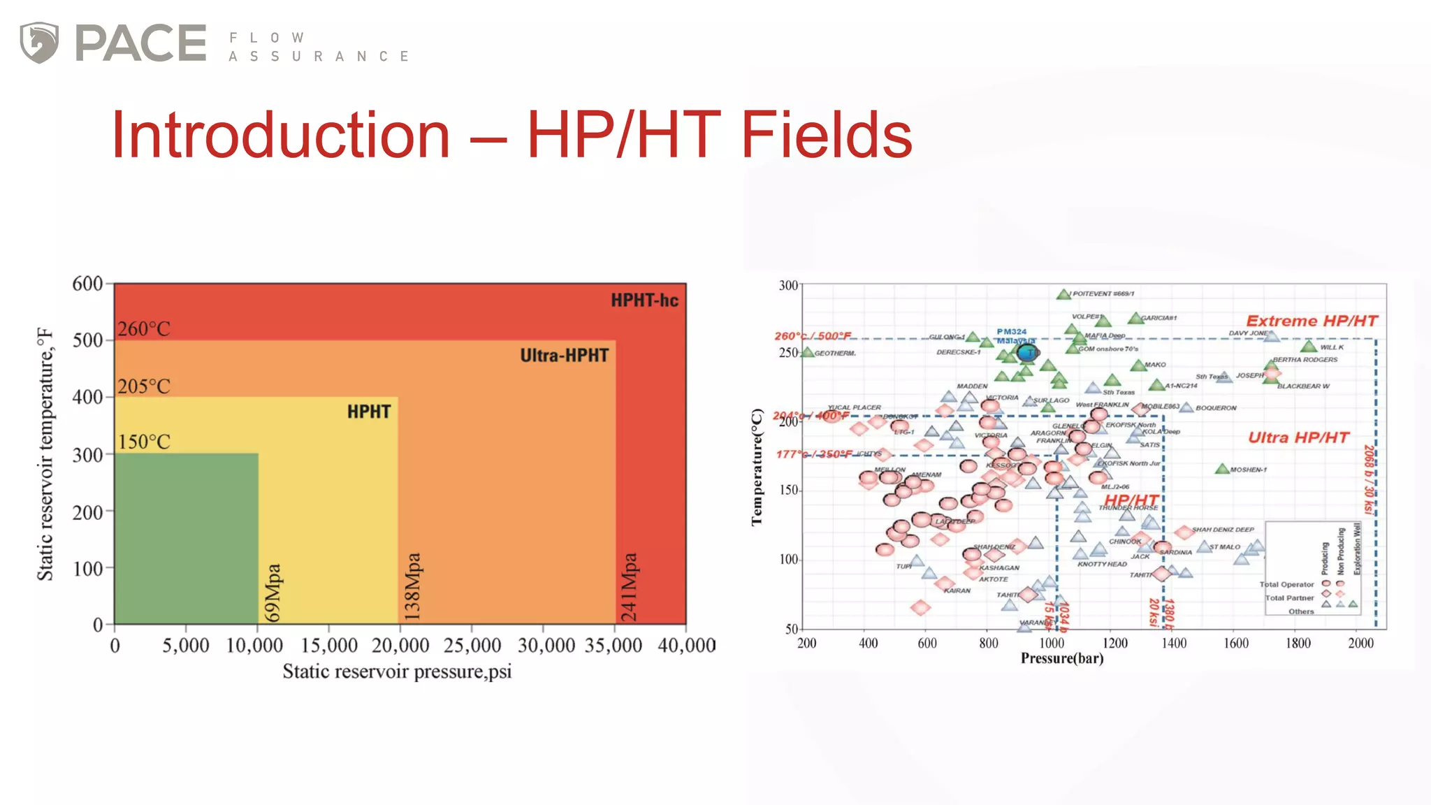
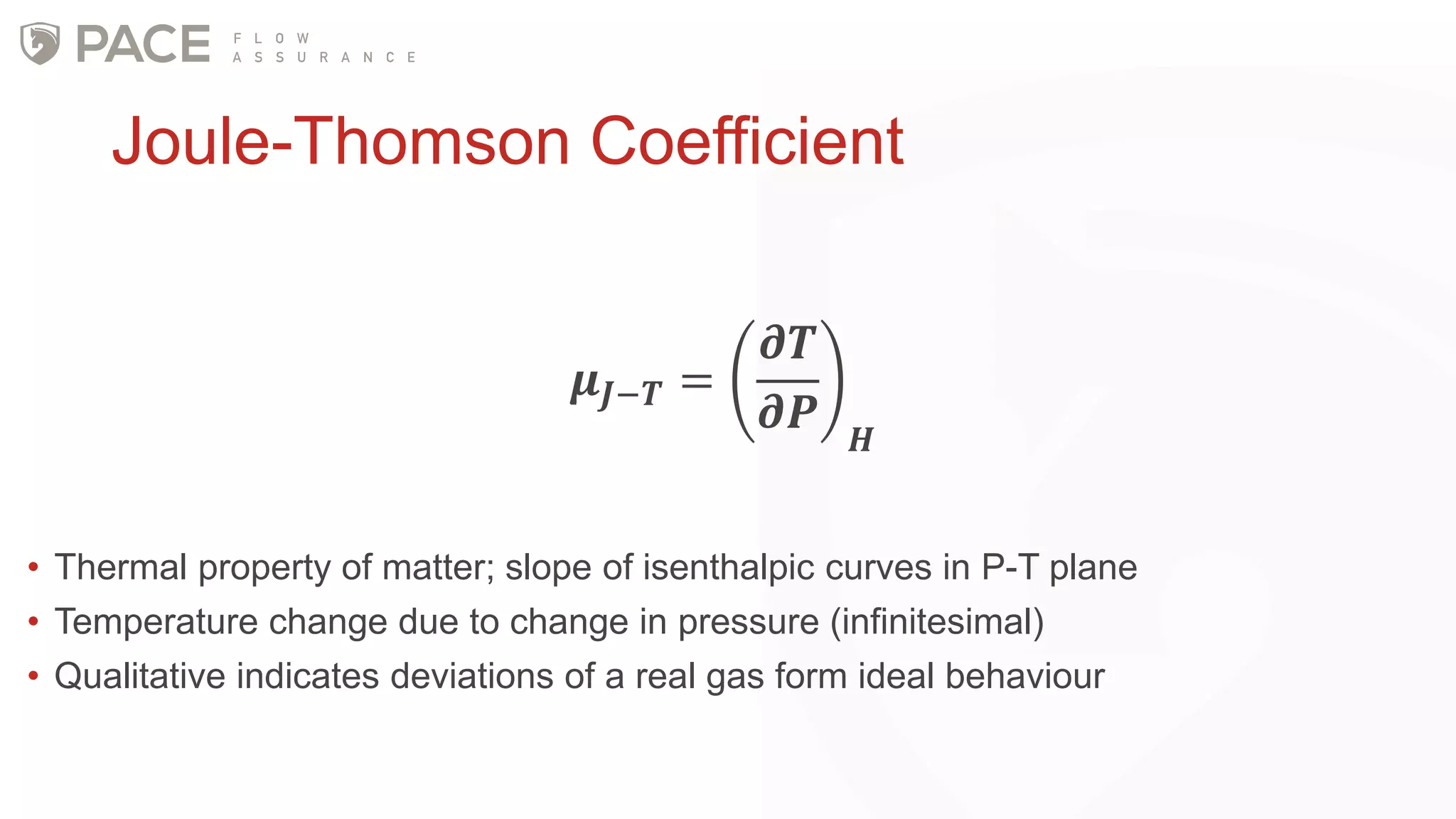
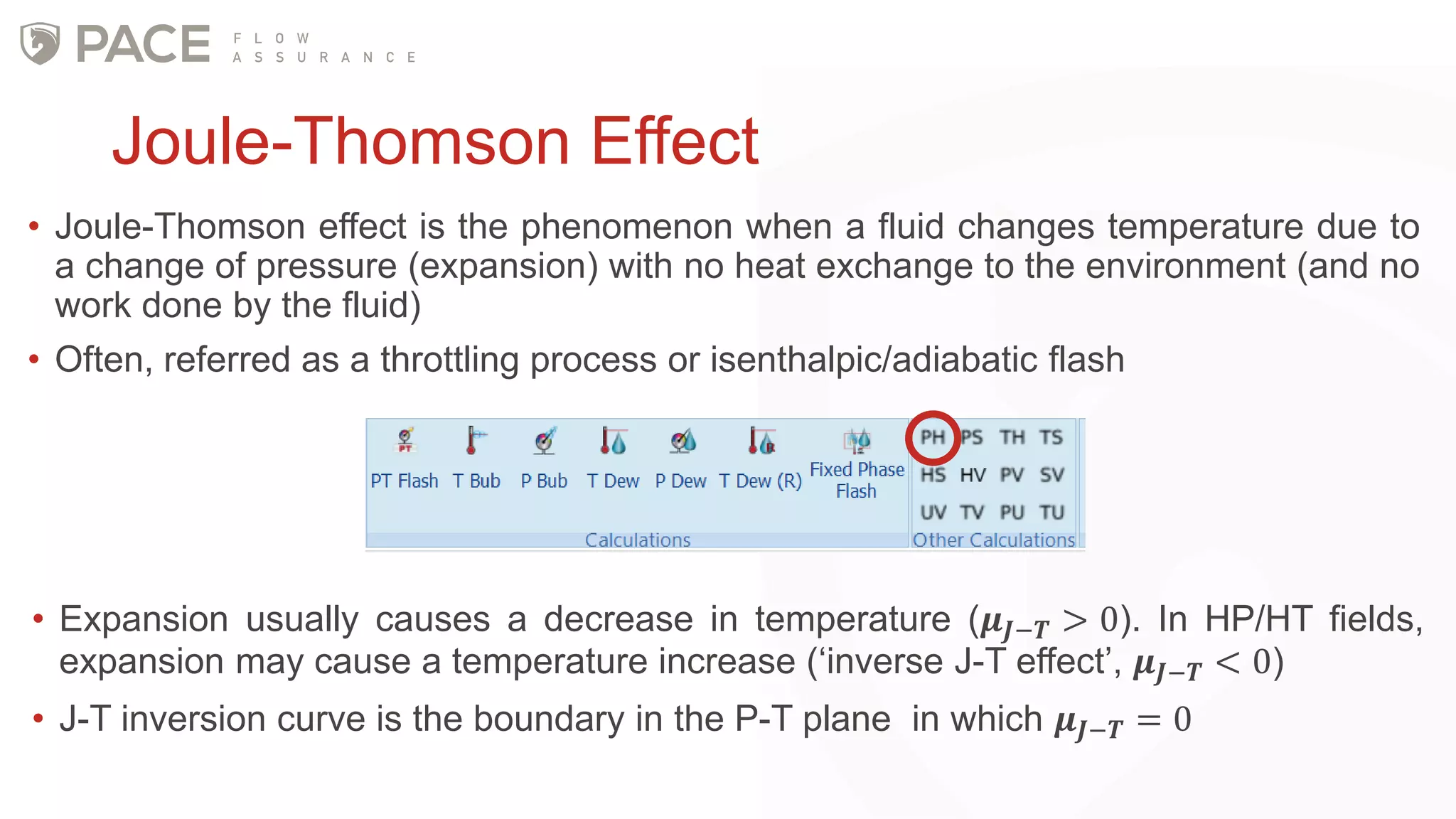
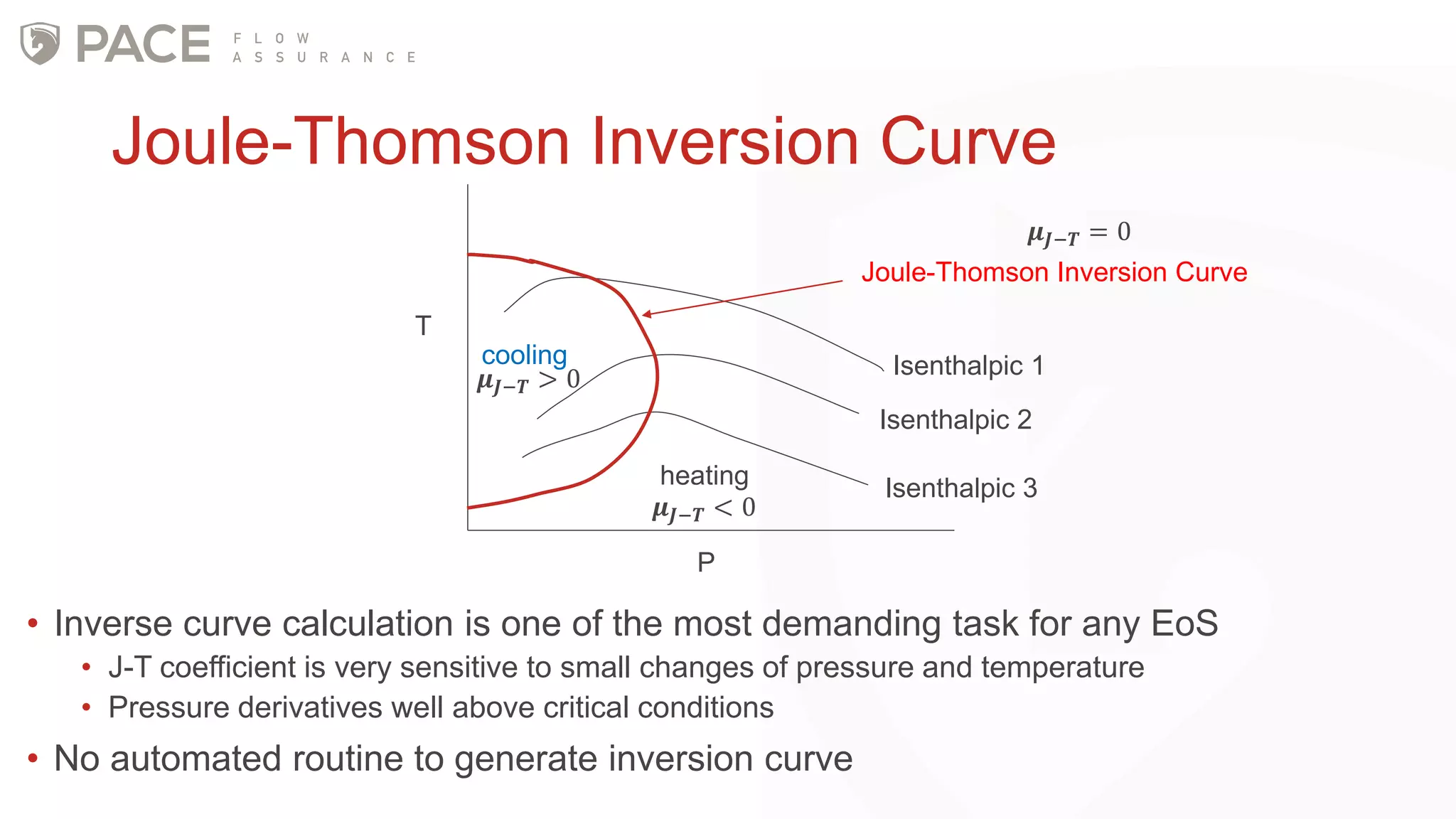
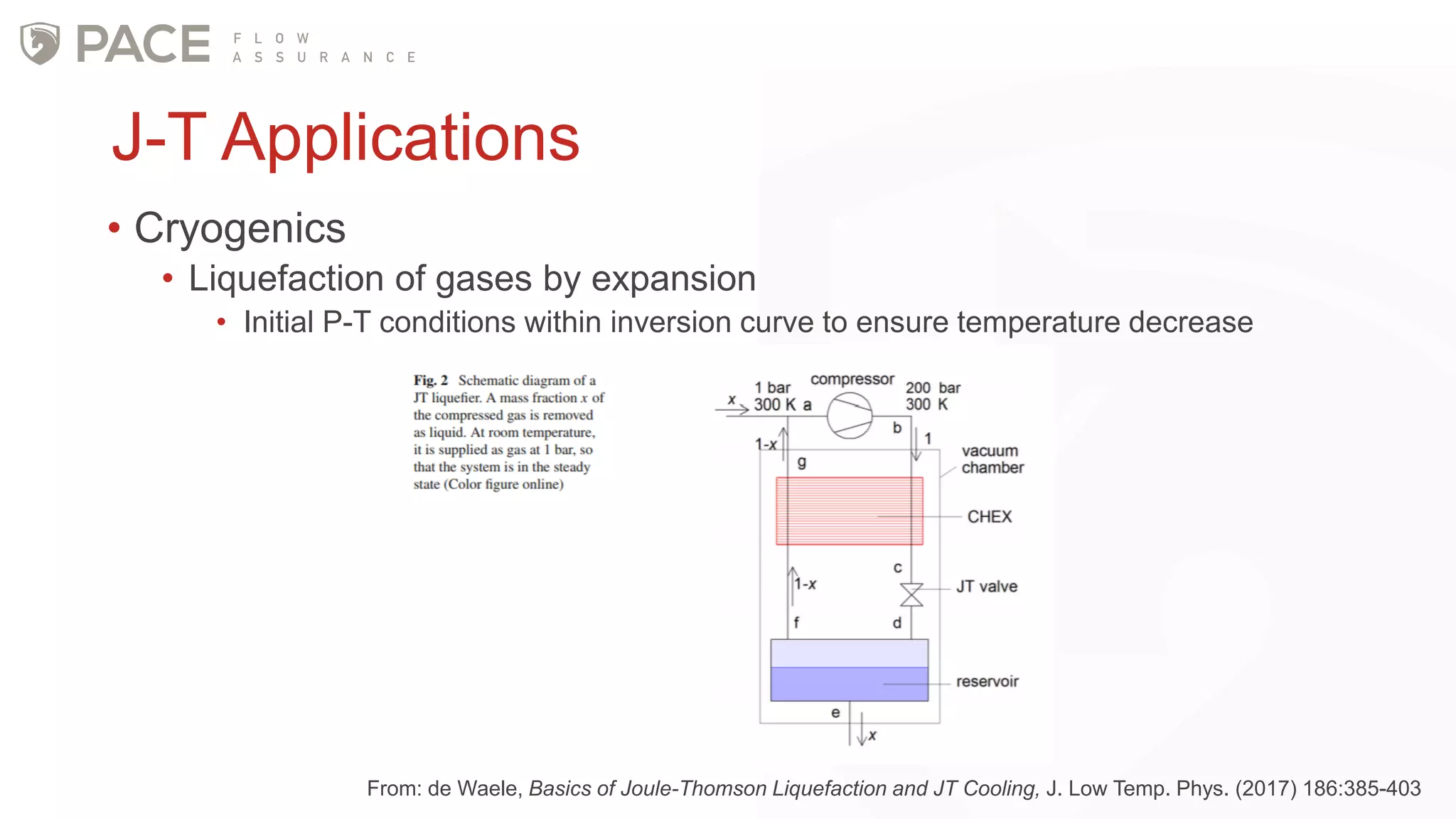
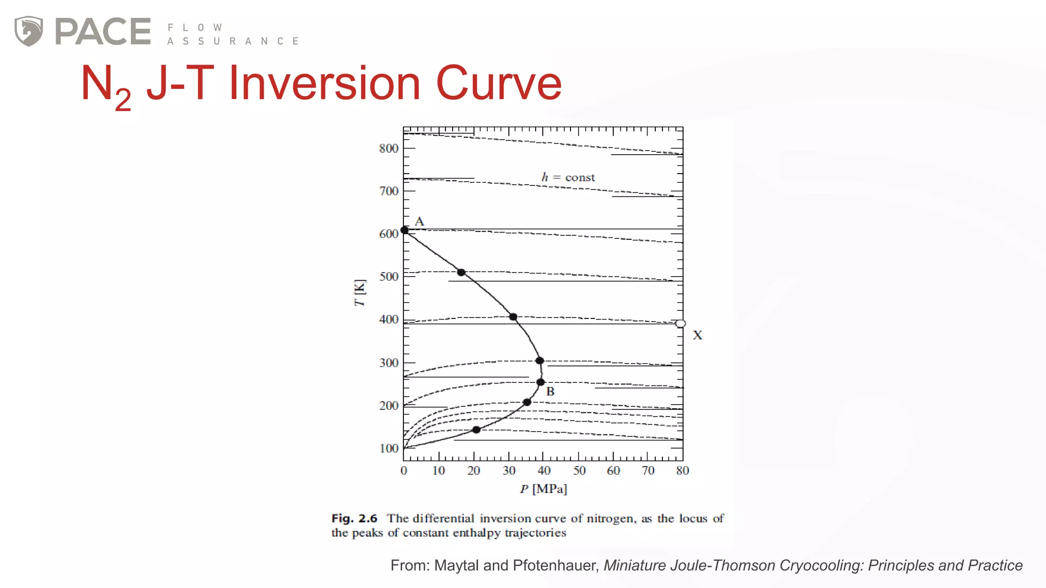
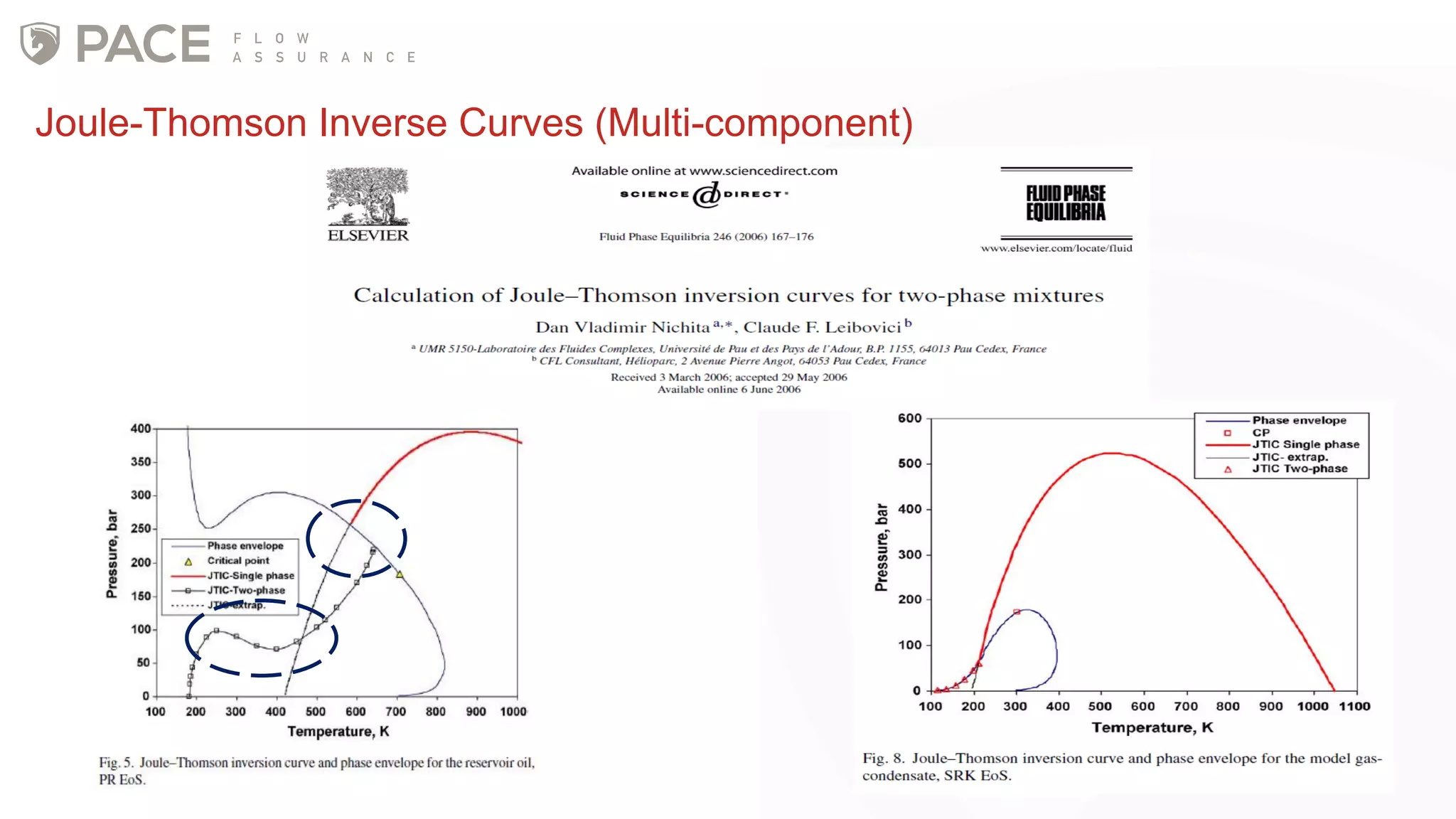
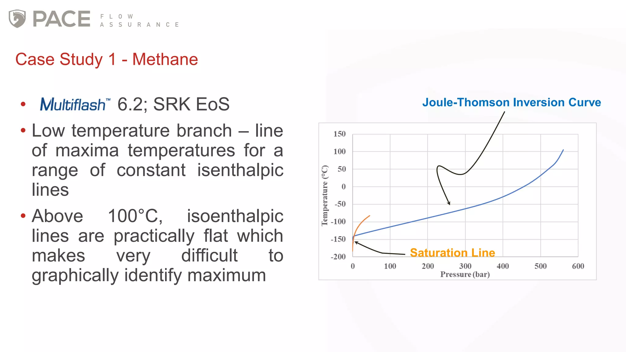
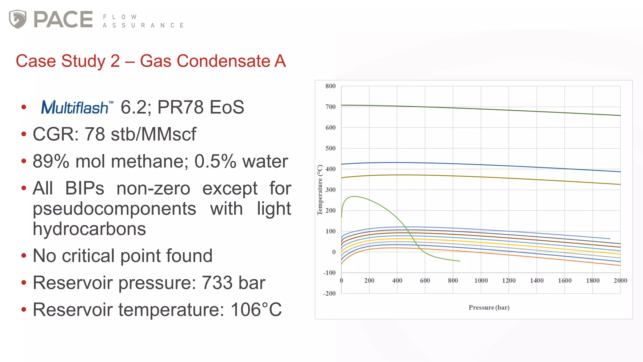
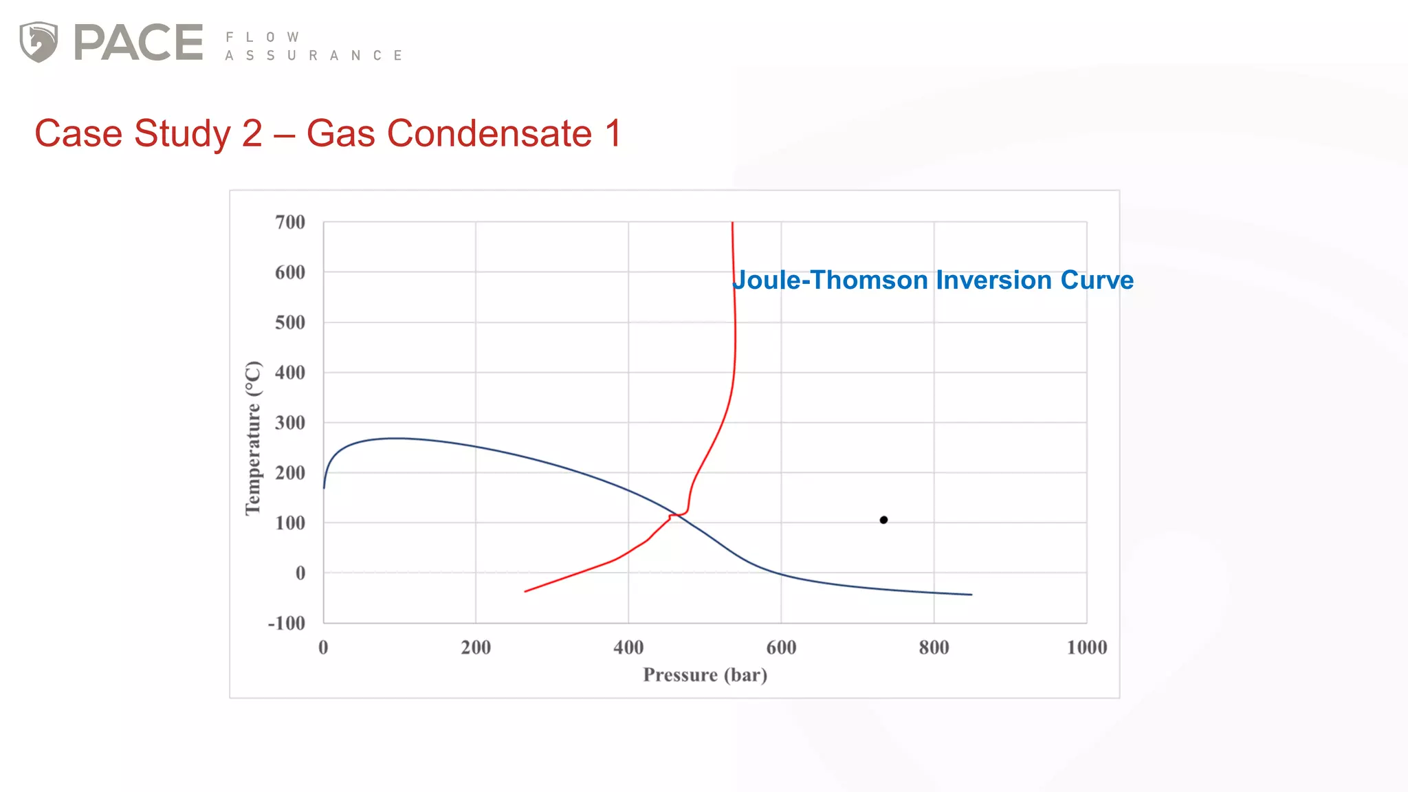
Thermodynamic behaviour of HPHT
reservoir fluids: Design considerations
during Joule-Thomson expansion
KBC Simulation Products User Conference
Europe, Africa and Middle East
18 June 2018
London, UK
Eduardo Luna-Ortiz
Pace Flow Assurance
eduardo@paceflowassurance.co.ukwww.paceflowassurance.co.uk
• Independent consultancy formed in 2017 based in Waterloo (London,
UK)
• Complete suite of flow assurance services including
• Fluid modelling
• IPM
• Production optimisation
• Ops and startup support
• High quality communication
• we work in a human way, to free engineers to do engineering
Outline
• Introduction and Motivation
• Joule-Thomson effect
• Applications
• Implications in upstream engineering
• Case studies
• Conclusions
Introduction – HP/HT Fields
Challenges HP/HT
• Drilling and Completion design
• Rigs are larger due to requirements such as hook load, mud pumps, drill pipe and surface
mud capacity
• Mud selection to be compatible to extreme P-T conditions
• Technology limitations and equipment selection
• Subsea equipment rated to high pressures
• Material selection
• Exotic alloys to withstand high temperatures
• Coating to be qualified to extreme conditions
• Safety issues
• HIPPS
• BOPs
Key Thermodynamic Properties under
HP/HT
• Density and viscosity key at in-situ reservoir conditions
• Water saturation / Gas solubility
• Compressibility
• Joule-Thomson coefficient
Joule-Thomson Coefficient
𝝁 𝑱−𝑻 =
𝝏𝑻
𝝏𝑷 𝑯
• Thermal property of matter; slope of isenthalpic curves in P-T plane
• Temperature change due to change in pressure (infinitesimal)
• Qualitative indicates deviations of a real gas form ideal behaviour
• James Joule
• Physicist / Mathematician / Brewer
• Conservation of energy (foundations
of First Law of Thermodynamics)
• William Thomson (Lord Kelvin)
• Physicist / Mathematician
• Yes, the one of the absolute
temperature scale (Kelvin scale)
Motivation
Joule-Thomson Effect
• Joule-Thomson effect is the phenomenon when a fluid changes temperature due to
a change of pressure (expansion) with no heat exchange to the environment (and no
work done by the fluid)
• Often, referred as a throttling process or isenthalpic/adiabatic flash
• Expansion usually causes a decrease in temperature (𝝁 𝑱−𝑻 > 0). In HP/HT fields,
expansion may cause a temperature increase (‘inverse J-T effect’, 𝝁 𝑱−𝑻 < 0)
• J-T inversion curve is the boundary in the P-T plane in which 𝝁 𝑱−𝑻 = 0
Joule-Thomson Inversion Curve
cooling
heating
T
P
Joule-Thomson Inversion Curve
Isenthalpic 3
Isenthalpic 2
Isenthalpic 1
• Inverse curve calculation is one of the most demanding task for any EoS
• J-T coefficient is very sensitive to small changes of pressure and temperature
• Pressure derivatives well above critical conditions
• No automated routine to generate inversion curve
𝝁 𝑱−𝑻 > 0
𝝁 𝑱−𝑻 < 0
𝝁 𝑱−𝑻 = 0
J-T Applications
• Cryogenics
• Liquefaction of gases by expansion
• Initial P-T conditions within inversion curve to ensure temperature decrease
From: de Waele, Basics of Joule-Thomson Liquefaction and JT Cooling, J. Low Temp. Phys. (2017) 186:385-403
J-T Effect in Oil & Gas
• dP across reservoir formation
• High drawdown can produce significant JT effect (heating)
• Completion material design
• Well testing
• J-T coefficient used to inferred bottom-hole conditions
• dP across production choke, PRV or orifice
• Hydrate formation
• Material design
• dP across multiphase meters
• Density correction (or other temperature dependent physical properties)
• CO2 sequestration
• HP CO2 expands into a relatively LP reservoir
N2 J-T Inversion Curve
From: Maytal and Pfotenhauer, Miniature Joule-Thomson Cryocooling: Principles and Practice
Joule-Thomson Inverse Curves (Multi-component)
• Inversion curves for pure components is well studied and published elsewhere for a
range of EoS and molecular simulation.
• Cubic EoS give good results for the low temperature branch but poor for the
maximum pressure and high temperature branch (SRK seems to performed better)
• 𝝁 𝑱−𝑻 =
𝝏𝑻
𝝏𝑷 𝑯
holds for a single-phase fluid. For mixture with phase splitting, the
definition must include contributions of both isenthalpic flash and phase split 𝝁 𝑱−𝑻∗ =𝝏𝑻
𝝏𝑷 𝑯𝒕
• Discontinuities appear as the inverse curve crosses the phase envelope. Multiple
temperature branches in the two-phase region.
• Nichita and Leibovici proposed several methods to determine the two-phase
inversion curves. In this work, we construct a ‘pseudo’ inverse curve based on
graphical method (line of maxima T for a range of isenthalpics).
• Can we detect discontinuities in the inverse curve?
• Define a pseudo J-T coefficient based on a volumetric average of the individual J-T
coefficient calculated by Multiflash
Challenges
Case Study 1 - Methane
Joule-Thomson Inversion Curve
Saturation Line
• 6.2; SRK EoS
• Low temperature branch – line
of maxima temperatures for a
range of constant isenthalpic
lines
• Above 100°C, isoenthalpic
lines are practically flat which
makes very difficult to
graphically identify maximum
Case Study 2 – Gas Condensate A
• 6.2; PR78 EoS
• CGR: 78 stb/MMscf
• 89% mol methane; 0.5% water
• All BIPs non-zero except for
pseudocomponents with light
hydrocarbons
• No critical point found
• Reservoir pressure: 733 bar
• Reservoir temperature: 106°C
Case Study 2 – Gas Condensate 1
Joule-Thomson Inversion Curve
Case Study 2 – Gas Condensate 1
• Discontinuity “found” in region
near to phase envelope
• Phase stability test ensures that
enthalpy calculation considers
phase splitting effect
• Green broken lines represent an
“interpolated” section from the
single-phase and two-phase
inversion curves to the saturation
line
Case Study 2 – Gas Condensate 1 • J-T coefficients at 122°C
• Multiflash mixture J-T coefficient
(mass) does not reflect discontinuity
across the phase change
• Volumetric J-T coefficient, 𝜇 𝐽−𝑇
𝑚
=
𝜌 𝐿 𝜇 𝐽−𝑇
𝐿
+𝜌 𝐺 𝜇 𝐽−𝑇
𝐺
𝜌 𝑚
, does capture
discontinuity across the phase
change
• 𝜇 𝐽−𝑇 =
𝑉
𝐶 𝑃
𝑇𝛼 − 1 , where 𝛼 is the
thermal expansion coefficient and a
discontinuity across the phase
change is expected
J-T coefficient
(Two-phase): MF (Mass)
J-T coefficient
(Single phase)
J-T coefficient
(Two-phase): Volumetric
Phase change
Case Study 3 – Gas Condensate B
• 6.0; CPA EoS
• CGR: 27 stb/MMscf
• 91% mol methane; 0.8% water
• All BIPs non-zero
• No critical point found
• Reservoir pressure: 879 bar
• Reservoir temperature: 133°C
• CITHP: 732 bar
• J-T heating due to reservoir drawdown was not considered in
Concept. Might have an impact in subsea design temperatures or
estimation of flowing wellhead temperatures.
• Negative J-T coefficient means that fluid will exhibit J-T heating while
positive coefficient means that the fluid will cooldown during
isenthalpic expansion. Heating across the bottom-hole is expected
during production up to the reservoir declines to a pressure of circa
550 bar.
• Increase is not very large for the expected reservoir drainage
(maximum 4°C increase). However, subsea design temperatures had
to be increased (re-qualification of some items was required)
• Expansion from 550 bar will lead to cooling rather than heating. It is
important to note that at 550 bar the reservoir is still in single phase.
• J-T inversion effect is not necessarily coincident with phase splitting.
Case Study 3 – Gas Condensate B
• JT effect across choke during well restart was also
investigated to verify that temperature D/S choke
does not transgress minimum design temperatures.
• To avoid excessive JT cooling, a high-pressure D/S
choke had to be imposed (80 bar). From CITHP
(732 bar) and ambient condition (13°C), the
resulting temperature after isenthalpic flash is -18°C
(minimum design temperature set to -29°C).
• JT cooling increases with decreasing CITHP (with
the same back-pressure D/S choke).
• Highest CITHP is not necessarily the governing
scenario for minimum design temperatures and/or
methanol requirements for hydrate mitigation
Case Study 3 – Gas Condensate B
CITHP
(bara)
Minimum Pressure D/S choke
(bara)
Minimum Temperature D/S choke
(°C)
725 65 -23.7
517 84 -23.7
466 85 -24.0
442 87 -23.6
Case Study 3 – Gas Condensate B
• Lower CITHP scenario dictates required restart pressure during
field life
• First start-up is not governing scenario
• Identify potential bottlenecks during field life
• Production technologists and reservoir
engineers require J-T coefficient for
calibration of Distributed Temperature
Sensing (DTS)
• Range of J-T coefficients were provided
• Note that two-phase J-T coefficients are
provided as per Multiflash
• It was reported some discrepancies when
the fluid was in two-phase region. At the
time, it was thought that it was possibly due
to the presence of water/salts
Case Study 3 – Gas Condensate B
Conclusions
• HP/HT fields shows particular challenges
• Material selection
• Safety issues
• Phase behaviour
• Significant value in performing a thermodynamic study of the fluid
• Validates PVT experiments
• Offers insights into potential problems within the expected operational envelope
• J-T inversion curves can provide governing operating/design conditions
• J-T effect is important
• J-T heating can have an impact in design temperatures
• Highest pressure of the system does not necessarily gives the coldest scenario during J-T
cooling

Europe User Conference: thermodynamic behaviour of HPHT reservoir fluids and design considerations

  • 1.
    Thermodynamic behaviour ofHPHT reservoir fluids: Design considerations during Joule-Thomson expansion KBC Simulation Products User Conference Europe, Africa and Middle East 18 June 2018 London, UK Eduardo Luna-Ortiz Pace Flow Assurance eduardo@paceflowassurance.co.ukwww.paceflowassurance.co.uk
  • 2.
    • Independent consultancyformed in 2017 based in Waterloo (London, UK) • Complete suite of flow assurance services including • Fluid modelling • IPM • Production optimisation • Ops and startup support • High quality communication • we work in a human way, to free engineers to do engineering
  • 3.
    Outline • Introduction andMotivation • Joule-Thomson effect • Applications • Implications in upstream engineering • Case studies • Conclusions
  • 4.
  • 5.
    Challenges HP/HT • Drillingand Completion design • Rigs are larger due to requirements such as hook load, mud pumps, drill pipe and surface mud capacity • Mud selection to be compatible to extreme P-T conditions • Technology limitations and equipment selection • Subsea equipment rated to high pressures • Material selection • Exotic alloys to withstand high temperatures • Coating to be qualified to extreme conditions • Safety issues • HIPPS • BOPs
  • 6.
    Key Thermodynamic Propertiesunder HP/HT • Density and viscosity key at in-situ reservoir conditions • Water saturation / Gas solubility • Compressibility • Joule-Thomson coefficient
  • 7.
    Joule-Thomson Coefficient 𝝁 𝑱−𝑻= 𝝏𝑻 𝝏𝑷 𝑯 • Thermal property of matter; slope of isenthalpic curves in P-T plane • Temperature change due to change in pressure (infinitesimal) • Qualitative indicates deviations of a real gas form ideal behaviour
  • 8.
    • James Joule •Physicist / Mathematician / Brewer • Conservation of energy (foundations of First Law of Thermodynamics) • William Thomson (Lord Kelvin) • Physicist / Mathematician • Yes, the one of the absolute temperature scale (Kelvin scale) Motivation
  • 9.
    Joule-Thomson Effect • Joule-Thomsoneffect is the phenomenon when a fluid changes temperature due to a change of pressure (expansion) with no heat exchange to the environment (and no work done by the fluid) • Often, referred as a throttling process or isenthalpic/adiabatic flash • Expansion usually causes a decrease in temperature (𝝁 𝑱−𝑻 > 0). In HP/HT fields, expansion may cause a temperature increase (‘inverse J-T effect’, 𝝁 𝑱−𝑻 < 0) • J-T inversion curve is the boundary in the P-T plane in which 𝝁 𝑱−𝑻 = 0
  • 10.
    Joule-Thomson Inversion Curve cooling heating T P Joule-ThomsonInversion Curve Isenthalpic 3 Isenthalpic 2 Isenthalpic 1 • Inverse curve calculation is one of the most demanding task for any EoS • J-T coefficient is very sensitive to small changes of pressure and temperature • Pressure derivatives well above critical conditions • No automated routine to generate inversion curve 𝝁 𝑱−𝑻 > 0 𝝁 𝑱−𝑻 < 0 𝝁 𝑱−𝑻 = 0
  • 11.
    J-T Applications • Cryogenics •Liquefaction of gases by expansion • Initial P-T conditions within inversion curve to ensure temperature decrease From: de Waele, Basics of Joule-Thomson Liquefaction and JT Cooling, J. Low Temp. Phys. (2017) 186:385-403
  • 12.
    J-T Effect inOil & Gas • dP across reservoir formation • High drawdown can produce significant JT effect (heating) • Completion material design • Well testing • J-T coefficient used to inferred bottom-hole conditions • dP across production choke, PRV or orifice • Hydrate formation • Material design • dP across multiphase meters • Density correction (or other temperature dependent physical properties) • CO2 sequestration • HP CO2 expands into a relatively LP reservoir
  • 13.
    N2 J-T InversionCurve From: Maytal and Pfotenhauer, Miniature Joule-Thomson Cryocooling: Principles and Practice
  • 14.
  • 15.
    • Inversion curvesfor pure components is well studied and published elsewhere for a range of EoS and molecular simulation. • Cubic EoS give good results for the low temperature branch but poor for the maximum pressure and high temperature branch (SRK seems to performed better) • 𝝁 𝑱−𝑻 = 𝝏𝑻 𝝏𝑷 𝑯 holds for a single-phase fluid. For mixture with phase splitting, the definition must include contributions of both isenthalpic flash and phase split 𝝁 𝑱−𝑻∗ =𝝏𝑻 𝝏𝑷 𝑯𝒕 • Discontinuities appear as the inverse curve crosses the phase envelope. Multiple temperature branches in the two-phase region. • Nichita and Leibovici proposed several methods to determine the two-phase inversion curves. In this work, we construct a ‘pseudo’ inverse curve based on graphical method (line of maxima T for a range of isenthalpics). • Can we detect discontinuities in the inverse curve? • Define a pseudo J-T coefficient based on a volumetric average of the individual J-T coefficient calculated by Multiflash Challenges
  • 16.
    Case Study 1- Methane Joule-Thomson Inversion Curve Saturation Line • 6.2; SRK EoS • Low temperature branch – line of maxima temperatures for a range of constant isenthalpic lines • Above 100°C, isoenthalpic lines are practically flat which makes very difficult to graphically identify maximum
  • 17.
    Case Study 2– Gas Condensate A • 6.2; PR78 EoS • CGR: 78 stb/MMscf • 89% mol methane; 0.5% water • All BIPs non-zero except for pseudocomponents with light hydrocarbons • No critical point found • Reservoir pressure: 733 bar • Reservoir temperature: 106°C
  • 18.
    Case Study 2– Gas Condensate 1 Joule-Thomson Inversion Curve
  • 19.
    Case Study 2– Gas Condensate 1 • Discontinuity “found” in region near to phase envelope • Phase stability test ensures that enthalpy calculation considers phase splitting effect • Green broken lines represent an “interpolated” section from the single-phase and two-phase inversion curves to the saturation line
  • 20.
    Case Study 2– Gas Condensate 1 • J-T coefficients at 122°C • Multiflash mixture J-T coefficient (mass) does not reflect discontinuity across the phase change • Volumetric J-T coefficient, 𝜇 𝐽−𝑇 𝑚 = 𝜌 𝐿 𝜇 𝐽−𝑇 𝐿 +𝜌 𝐺 𝜇 𝐽−𝑇 𝐺 𝜌 𝑚 , does capture discontinuity across the phase change • 𝜇 𝐽−𝑇 = 𝑉 𝐶 𝑃 𝑇𝛼 − 1 , where 𝛼 is the thermal expansion coefficient and a discontinuity across the phase change is expected J-T coefficient (Two-phase): MF (Mass) J-T coefficient (Single phase) J-T coefficient (Two-phase): Volumetric Phase change
  • 21.
    Case Study 3– Gas Condensate B • 6.0; CPA EoS • CGR: 27 stb/MMscf • 91% mol methane; 0.8% water • All BIPs non-zero • No critical point found • Reservoir pressure: 879 bar • Reservoir temperature: 133°C • CITHP: 732 bar
  • 22.
    • J-T heatingdue to reservoir drawdown was not considered in Concept. Might have an impact in subsea design temperatures or estimation of flowing wellhead temperatures. • Negative J-T coefficient means that fluid will exhibit J-T heating while positive coefficient means that the fluid will cooldown during isenthalpic expansion. Heating across the bottom-hole is expected during production up to the reservoir declines to a pressure of circa 550 bar. • Increase is not very large for the expected reservoir drainage (maximum 4°C increase). However, subsea design temperatures had to be increased (re-qualification of some items was required) • Expansion from 550 bar will lead to cooling rather than heating. It is important to note that at 550 bar the reservoir is still in single phase. • J-T inversion effect is not necessarily coincident with phase splitting. Case Study 3 – Gas Condensate B
  • 23.
    • JT effectacross choke during well restart was also investigated to verify that temperature D/S choke does not transgress minimum design temperatures. • To avoid excessive JT cooling, a high-pressure D/S choke had to be imposed (80 bar). From CITHP (732 bar) and ambient condition (13°C), the resulting temperature after isenthalpic flash is -18°C (minimum design temperature set to -29°C). • JT cooling increases with decreasing CITHP (with the same back-pressure D/S choke). • Highest CITHP is not necessarily the governing scenario for minimum design temperatures and/or methanol requirements for hydrate mitigation Case Study 3 – Gas Condensate B
  • 24.
    CITHP (bara) Minimum Pressure D/Schoke (bara) Minimum Temperature D/S choke (°C) 725 65 -23.7 517 84 -23.7 466 85 -24.0 442 87 -23.6 Case Study 3 – Gas Condensate B • Lower CITHP scenario dictates required restart pressure during field life • First start-up is not governing scenario • Identify potential bottlenecks during field life
  • 25.
    • Production technologistsand reservoir engineers require J-T coefficient for calibration of Distributed Temperature Sensing (DTS) • Range of J-T coefficients were provided • Note that two-phase J-T coefficients are provided as per Multiflash • It was reported some discrepancies when the fluid was in two-phase region. At the time, it was thought that it was possibly due to the presence of water/salts Case Study 3 – Gas Condensate B
  • 26.
    Conclusions • HP/HT fieldsshows particular challenges • Material selection • Safety issues • Phase behaviour • Significant value in performing a thermodynamic study of the fluid • Validates PVT experiments • Offers insights into potential problems within the expected operational envelope • J-T inversion curves can provide governing operating/design conditions • J-T effect is important • J-T heating can have an impact in design temperatures • Highest pressure of the system does not necessarily gives the coldest scenario during J-T cooling