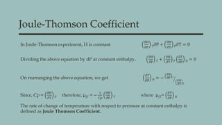
THERMODYNAMICS
Pallavi Kumbhar
MSc Part-I
CONTENTS
01 Maxwell’s Thermodynamic Relations
02 Common Forms of Maxwell’s Relations
03 State functions & Exact differentials
04 Joule Thomson Experiment
05 Joule-Thomson Coefficient
06 Significance of Joule-Thomson Coefficient
07 Joule-Thomson Coefficient For An Ideal Gas
08 Applications of Joule-Thomson Effect
Maxwells Thermodynamic Relations
What are Maxwell’s relations?
 These are the set of thermodynamics equations derived from a symmetry
of secondary derivatives and from thermodynamic potentials.
 For example dU = TdS – PdV
Then,
𝜕2
U
𝜕S𝜕V
=
𝜕T
𝜕V S = −
𝜕P
𝜕S V
 These relations are named after James Clerk Maxwell, who was a 19th-
century physicist.
Function Differential
Natural
Variables
Maxwell Relation
U dU = TdS – PdV S, V
𝜕T
𝜕V S = −
𝜕P
𝜕S V
H dH = TdS + VdP S, P
𝜕T
𝜕P S =
𝜕V
𝜕S P
A dA = -PdV – SdT V, T
𝜕P
𝜕T V =
𝜕S
𝜕V T
G dG = VdP – SdT P, T
𝜕V
𝜕T P = −
𝜕S
𝜕P T
Common Forms Of Maxwell’s Relations
Internal energy (U), Enthalpy (H), Helmholtz free energy (A), and Gibbs free energy
(G), entropy (S), pressure (P), volume (V), and temperature (T).
State Functions & Exact
Differentials
 State function is a property which depends only on the initial and final states of the
system and is independent of its path. Examples: U, H, S, A, G
 Exact differential is an infinitesimal quantity, which when integrated, gives a result
that is independent of the path between the initial and final states.
 For example consider the function A(x, y) as an exact differential, where x and y are
independent variables
Then,
𝛛𝟐
𝐀
𝛛𝐲𝛛𝐱
=
𝛛𝟐
𝐀
𝛛𝐱𝛛𝐲
Or
𝛛𝟐
𝐀
𝛛𝐲𝛛𝐱
+
𝛛𝟐
𝐀
𝛛𝐱𝛛𝐲
= 𝐂 where C is arbitrary constant
Joule Thomson
Experiment
A B
T1 T2
P1>P2
The work done by piston A = P1V1
The work done by piston B = - P2V2
Net work done by the system, W = P1V1- P2V2
Change in internal energy, ∆U = U2- U1
From 1st law ∆U = q - w
Since q = 0, -∆U = -W
Substituting the values of ∆U and W we get,
-(P1V1- P2V2) = -(U2- U1)
P2V2 - P1V1 = U1- U2
Rearranging the terms, we get
U2 + P2V2 = U1 + P1V1
Since H = U + PV
Therefore, H2 = H1 and ∆H = 0
Thus, during Joule Thomson effect, enthalpy of the
system remains constant. It is also called Iso-
Joule-Thomson Coefficient
In Joule-Thomson experiment, H is constant
𝜕H
𝜕P T𝜕P +
𝜕H
𝜕T P𝜕T = 0
Dividing the above equation by dP at constant enthalpy,
𝜕H
𝜕P T +
𝜕H
𝜕T P
𝜕T
𝜕P H = 0
On rearranging the above equation, we get
𝜕T
𝜕P H = −
𝜕H
𝜕P T
𝜕H
𝜕T P
Since, Cp =
𝜕H
𝜕T P therefore, μJT = −
1
Cp
𝜕H
𝜕P T where μJT=
𝜕T
𝜕P H
The rate of change of temperature with respect to pressure at constant enthalpy is
defined as Joule Thomson Coefficient.
Significance Of Joule-Thomson Coefficient
If the gas
temperature is
then μJT is since ∂P is So the gas
above the
inversion
temperature
negative always negative warms
below the
inversion
temperature
positive always negative cools
The temperature at which µ=0 and the gas shows neither heating effect nor
cooling effect on adiabatic expansion is defined as inversion temperature.
Temperature Inversion Curve
In this curve…
1. Within the region bounded by the red line, a
Joule–Thomson expansion produces cooling
(μJT > 0).
2. Outside that region, the expansion produces
heating.
3. The gas–liquid coexistence curve is shown by
the blue line, terminating at the critical point
(the solid blue circle).
4. The dashed lines shows the regions where N2 is
neither a supercritical fluid, a liquid, nor a gas.
Joule-Thomson Coefficient For An Ideal
Gas
We know that, μJT = −
1
Cp
𝜕H
𝜕P T =
𝜕T
𝜕P H
Therefore, , μJT = −
1
Cp
𝜕(U+PV)
𝜕P T …(Since, H = U +
PV)
= −
1
Cp
[
𝜕U
𝜕P T +
𝜕(PV)
𝜕P T ]
= −
1
Cp
[
𝜕U
𝜕V T
𝜕V
𝜕P T +
𝜕(PV)
𝜕P T ]
For an ideal gas,
𝜕U
𝜕V T = 0
Also, PV = constant so,
𝜕(PV)
𝜕P T = 0
Therefore, μJT = 0
Applications of Joule-Thomson Effect
1. The cooling produced in the Joule-Thomson expansion has made it a very valuable
tool in refrigeration.
2. This effect is applied in the Linde technique in the petrochemical industry, where
the cooling effect is used to liquefy gases.
3. It is also used in many cryogenic applications. For example for the production of
liquid nitrogen, oxygen, and argon.
4. The effect can also be used to liquefy even helium.
REFRENCES
 Physical Chemistry Peter Atkins, Julio De Paula
 Images from Google
Thermodynamics

Thermodynamics

  • 1.
  • 2.
    CONTENTS 01 Maxwell’s ThermodynamicRelations 02 Common Forms of Maxwell’s Relations 03 State functions & Exact differentials 04 Joule Thomson Experiment 05 Joule-Thomson Coefficient 06 Significance of Joule-Thomson Coefficient 07 Joule-Thomson Coefficient For An Ideal Gas 08 Applications of Joule-Thomson Effect
  • 3.
    Maxwells Thermodynamic Relations Whatare Maxwell’s relations?  These are the set of thermodynamics equations derived from a symmetry of secondary derivatives and from thermodynamic potentials.  For example dU = TdS – PdV Then, 𝜕2 U 𝜕S𝜕V = 𝜕T 𝜕V S = − 𝜕P 𝜕S V  These relations are named after James Clerk Maxwell, who was a 19th- century physicist.
  • 4.
    Function Differential Natural Variables Maxwell Relation UdU = TdS – PdV S, V 𝜕T 𝜕V S = − 𝜕P 𝜕S V H dH = TdS + VdP S, P 𝜕T 𝜕P S = 𝜕V 𝜕S P A dA = -PdV – SdT V, T 𝜕P 𝜕T V = 𝜕S 𝜕V T G dG = VdP – SdT P, T 𝜕V 𝜕T P = − 𝜕S 𝜕P T Common Forms Of Maxwell’s Relations Internal energy (U), Enthalpy (H), Helmholtz free energy (A), and Gibbs free energy (G), entropy (S), pressure (P), volume (V), and temperature (T).
  • 5.
    State Functions &Exact Differentials  State function is a property which depends only on the initial and final states of the system and is independent of its path. Examples: U, H, S, A, G  Exact differential is an infinitesimal quantity, which when integrated, gives a result that is independent of the path between the initial and final states.  For example consider the function A(x, y) as an exact differential, where x and y are independent variables Then, 𝛛𝟐 𝐀 𝛛𝐲𝛛𝐱 = 𝛛𝟐 𝐀 𝛛𝐱𝛛𝐲 Or 𝛛𝟐 𝐀 𝛛𝐲𝛛𝐱 + 𝛛𝟐 𝐀 𝛛𝐱𝛛𝐲 = 𝐂 where C is arbitrary constant
  • 6.
    Joule Thomson Experiment A B T1T2 P1>P2 The work done by piston A = P1V1 The work done by piston B = - P2V2 Net work done by the system, W = P1V1- P2V2 Change in internal energy, ∆U = U2- U1 From 1st law ∆U = q - w Since q = 0, -∆U = -W Substituting the values of ∆U and W we get, -(P1V1- P2V2) = -(U2- U1) P2V2 - P1V1 = U1- U2 Rearranging the terms, we get U2 + P2V2 = U1 + P1V1 Since H = U + PV Therefore, H2 = H1 and ∆H = 0 Thus, during Joule Thomson effect, enthalpy of the system remains constant. It is also called Iso-
  • 7.
    Joule-Thomson Coefficient In Joule-Thomsonexperiment, H is constant 𝜕H 𝜕P T𝜕P + 𝜕H 𝜕T P𝜕T = 0 Dividing the above equation by dP at constant enthalpy, 𝜕H 𝜕P T + 𝜕H 𝜕T P 𝜕T 𝜕P H = 0 On rearranging the above equation, we get 𝜕T 𝜕P H = − 𝜕H 𝜕P T 𝜕H 𝜕T P Since, Cp = 𝜕H 𝜕T P therefore, μJT = − 1 Cp 𝜕H 𝜕P T where μJT= 𝜕T 𝜕P H The rate of change of temperature with respect to pressure at constant enthalpy is defined as Joule Thomson Coefficient.
  • 8.
    Significance Of Joule-ThomsonCoefficient If the gas temperature is then μJT is since ∂P is So the gas above the inversion temperature negative always negative warms below the inversion temperature positive always negative cools The temperature at which µ=0 and the gas shows neither heating effect nor cooling effect on adiabatic expansion is defined as inversion temperature.
  • 9.
    Temperature Inversion Curve Inthis curve… 1. Within the region bounded by the red line, a Joule–Thomson expansion produces cooling (μJT > 0). 2. Outside that region, the expansion produces heating. 3. The gas–liquid coexistence curve is shown by the blue line, terminating at the critical point (the solid blue circle). 4. The dashed lines shows the regions where N2 is neither a supercritical fluid, a liquid, nor a gas.
  • 10.
    Joule-Thomson Coefficient ForAn Ideal Gas We know that, μJT = − 1 Cp 𝜕H 𝜕P T = 𝜕T 𝜕P H Therefore, , μJT = − 1 Cp 𝜕(U+PV) 𝜕P T …(Since, H = U + PV) = − 1 Cp [ 𝜕U 𝜕P T + 𝜕(PV) 𝜕P T ] = − 1 Cp [ 𝜕U 𝜕V T 𝜕V 𝜕P T + 𝜕(PV) 𝜕P T ] For an ideal gas, 𝜕U 𝜕V T = 0 Also, PV = constant so, 𝜕(PV) 𝜕P T = 0 Therefore, μJT = 0
  • 11.
    Applications of Joule-ThomsonEffect 1. The cooling produced in the Joule-Thomson expansion has made it a very valuable tool in refrigeration. 2. This effect is applied in the Linde technique in the petrochemical industry, where the cooling effect is used to liquefy gases. 3. It is also used in many cryogenic applications. For example for the production of liquid nitrogen, oxygen, and argon. 4. The effect can also be used to liquefy even helium.
  • 12.
    REFRENCES  Physical ChemistryPeter Atkins, Julio De Paula  Images from Google