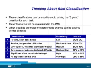
Downloaded 16 times

![Some Sobering Observations
In 1979, Tversky and Kahneman proposed an alternative to utility
theory. Prospect theory asserts that people make predictably irrational
decisions. [45], [52]
The way that a choice of decisions is presented can sway a person to
choose the less rational decision from a set of options.
Once a problem is clearly and reasonably presented, rarely does a
person think outside the bounds of the frame.
Source:
– “The Causes of Risk Taking By Project Managers,” Proceedings of
the Project Management Institute Annual Seminars & Symposium
November 1–10, 2001 • Nashville, Tenn
– Tversky, Amos, and Daniel Kahneman. 1981. The Framing of
Decisions and the Psychology of Choice. Science 211 (January 30):
453–458
27/41](https://image.slidesharecdn.com/establishingschedulemarginusingmontecarlosimulaitonv2-190317233239/85/Establishing-schedule-margin-using-monte-carlo-simulation-27-320.jpg)
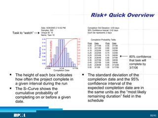
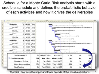
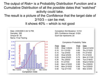
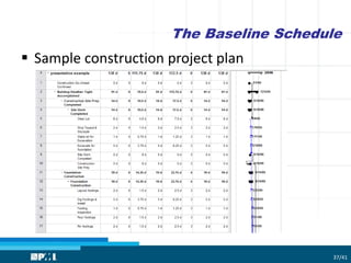
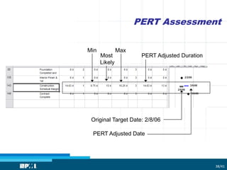
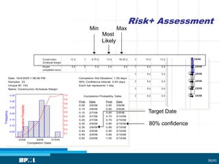
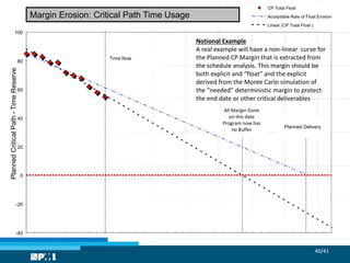

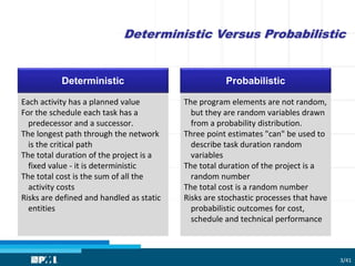
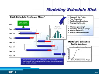
The document focuses on utilizing Monte Carlo simulation to identify schedule margins and manage uncertainties within project scheduling. It contrasts deterministic and probabilistic approaches to scheduling, emphasizing the necessity for proper integration of risk assessments in developing a credible project timeline. Key issues with traditional estimating methods are discussed, highlighting the flaws in single-point estimates and the importance of understanding underlying probability distributions for project duration.