Download as PDF, PPTX
![DSS framework
CMS 2016
Emilio L. Cano
An Integrated
Framework
Stochastic
Models
Conclusions
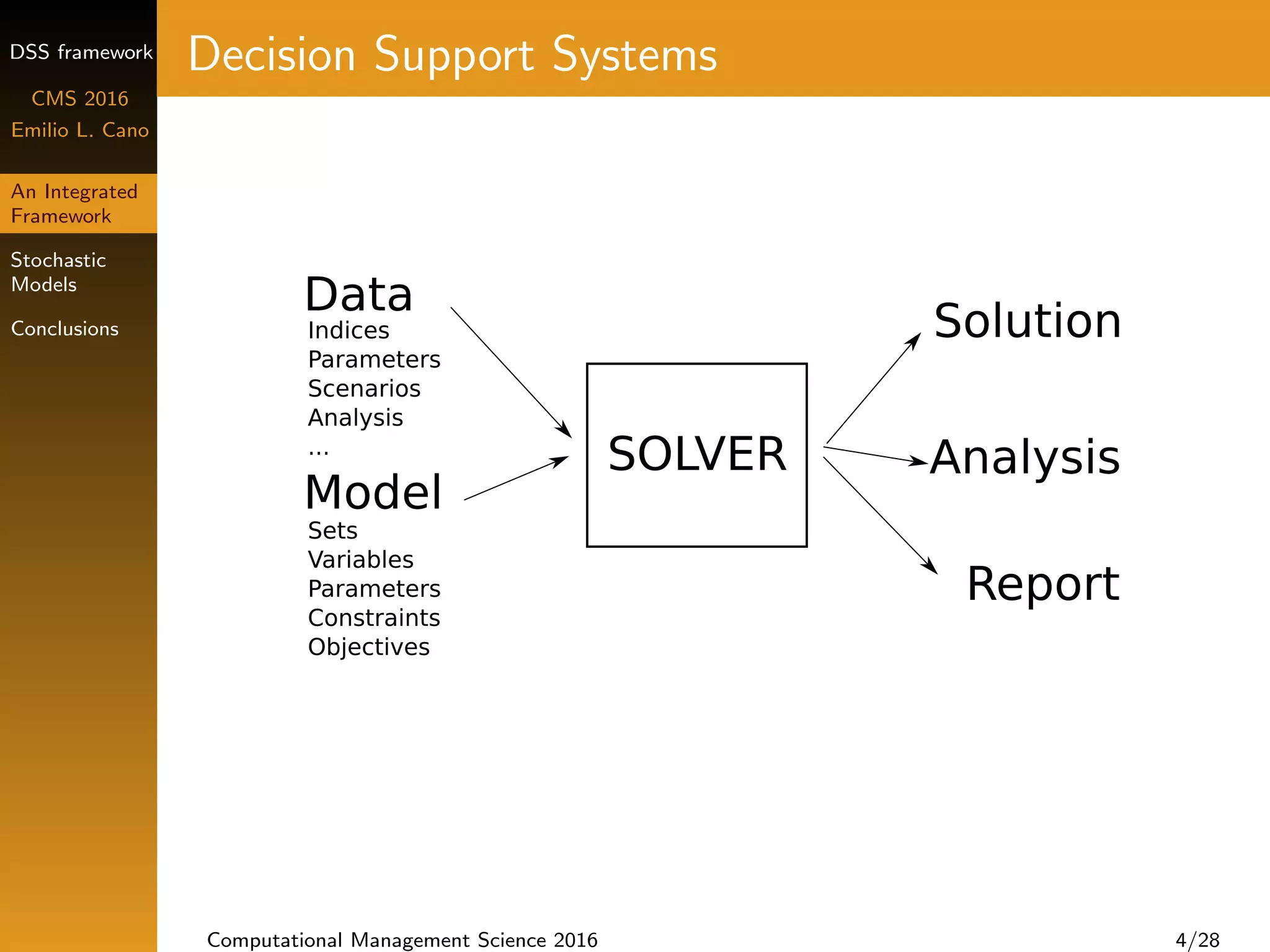
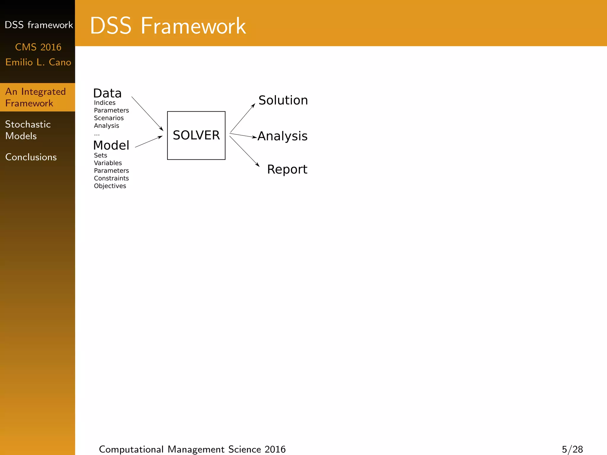
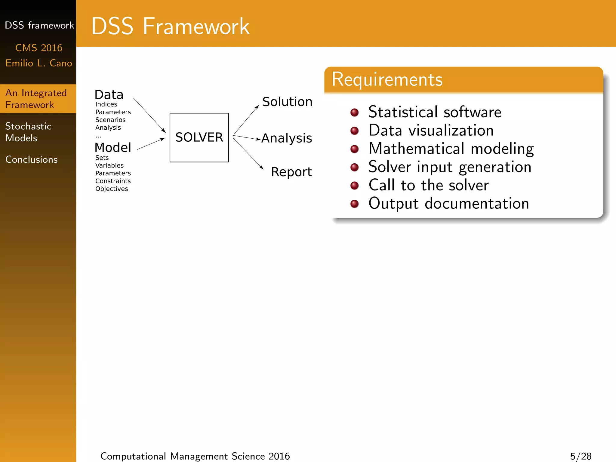
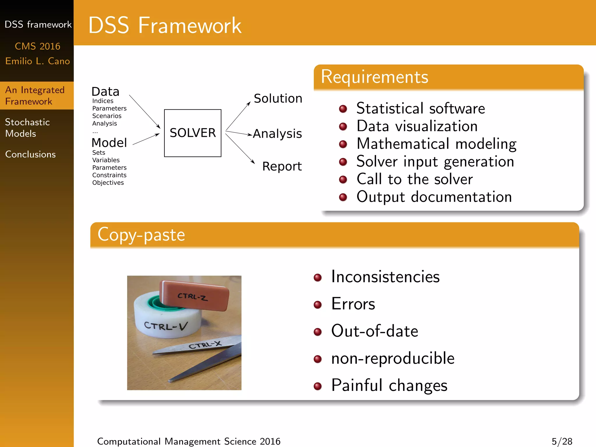
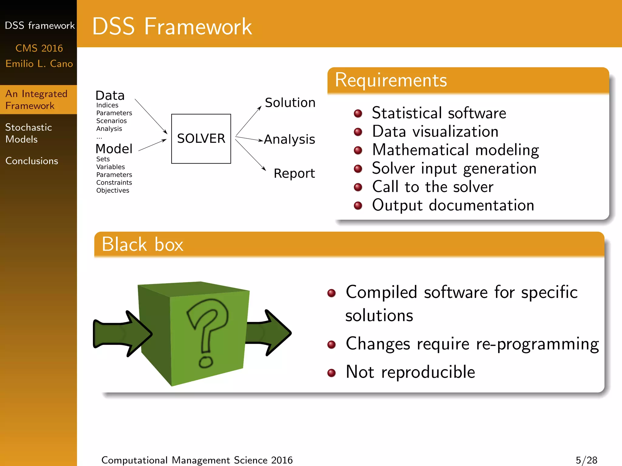
DSS Framework
Requirements
Statistical software
Data visualization
Mathematical modeling
Solver input generation
Call to the solver
Output documentation
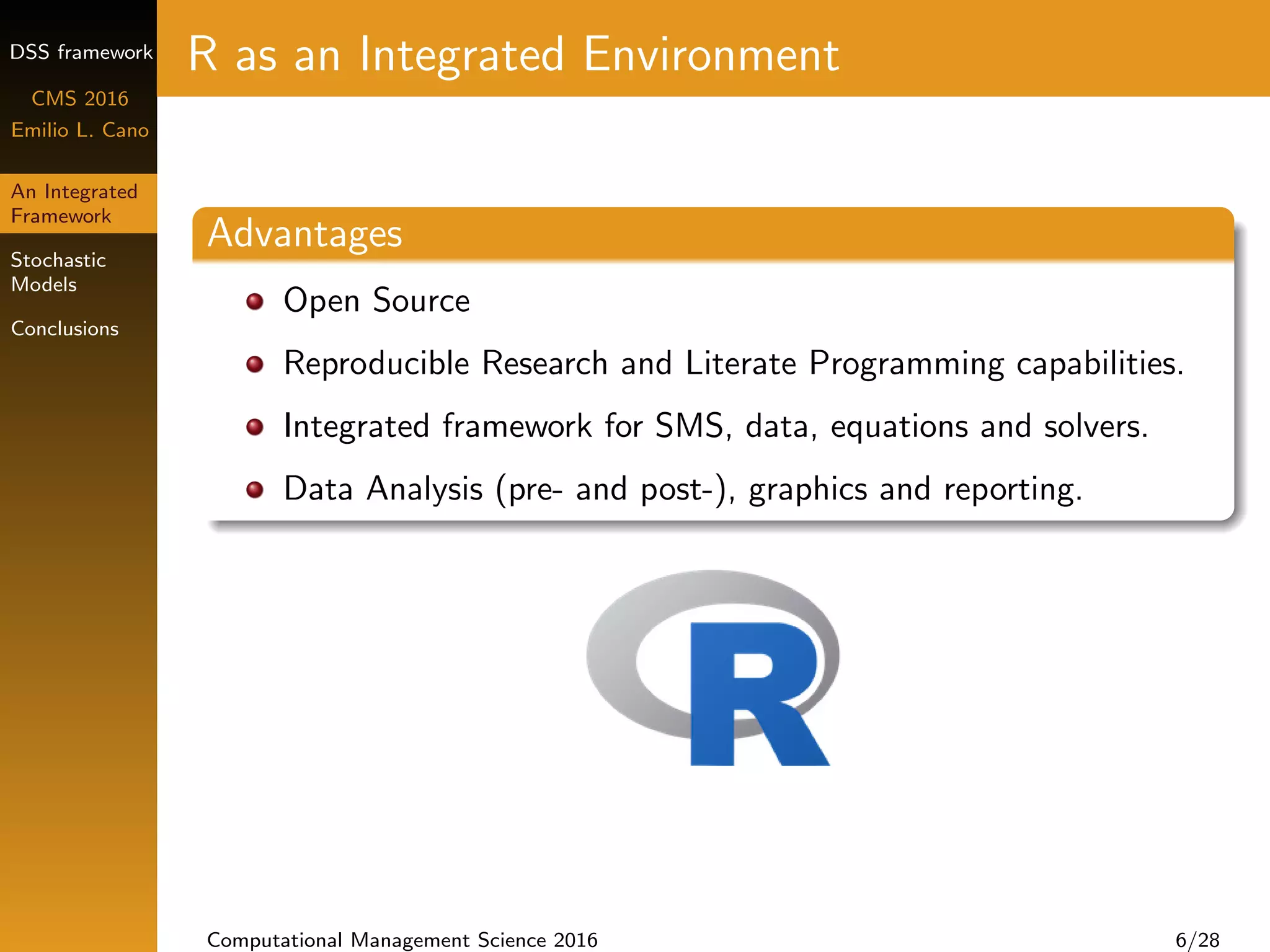
Framework
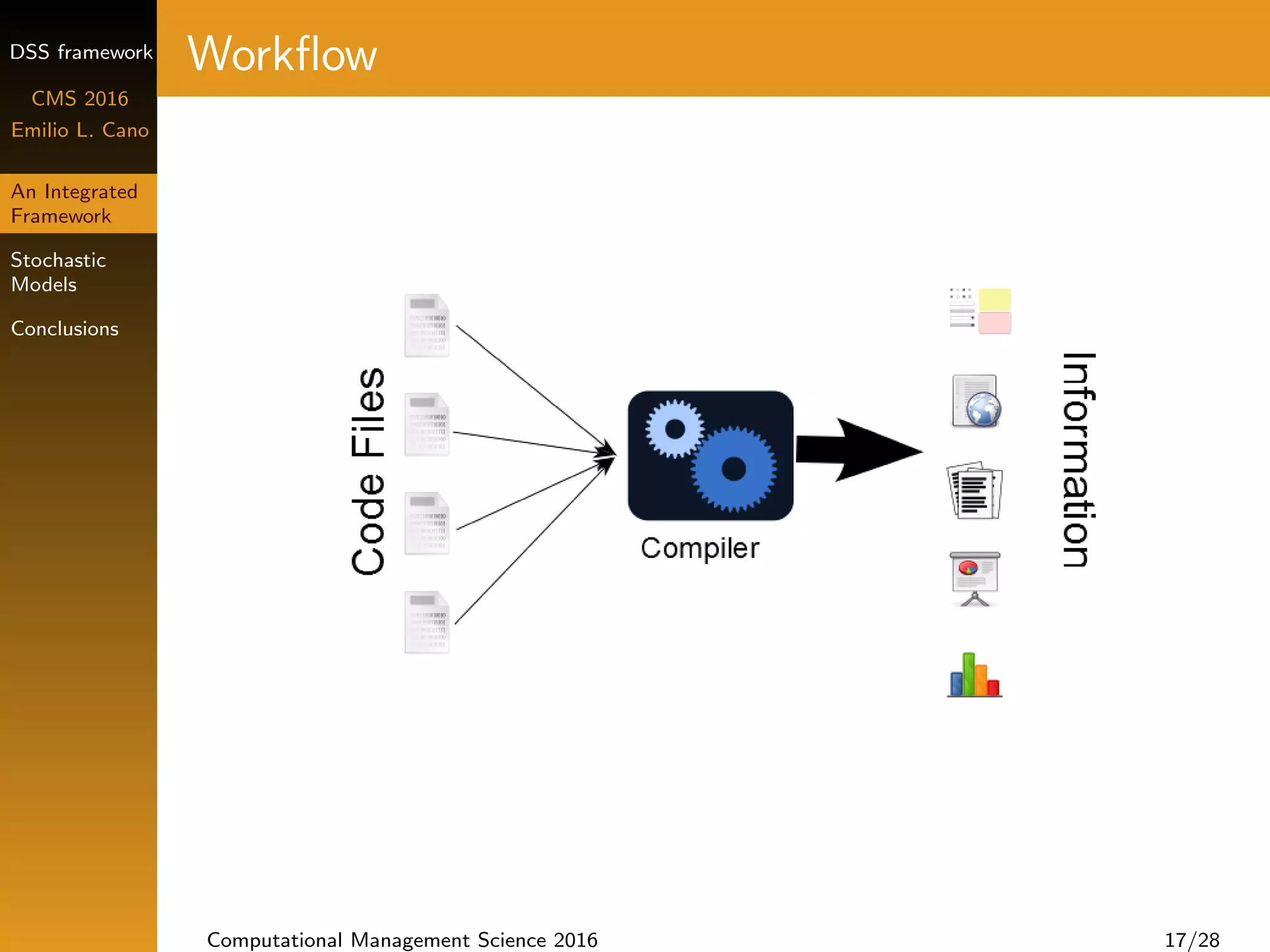
Reproducible Research & Literate Programming
omptimr R package & Algebraic Modeling Languages (AMLs)
“The goal of RR is to tie specific instructions to data analysis and
experimental data [and modeling] so that results can be recreated,
better understood and verified”
“LP: a document that is a combination of content and data analysis
code [and models]”
Computational Management Science 2016 5/28](https://image.slidesharecdn.com/elcanocms2016slides-160805093244/75/Energy-efficient-technology-investments-using-a-decision-support-system-framework-11-2048.jpg)
![DSS framework
CMS 2016
Emilio L. Cano
An Integrated
Framework
Stochastic
Models
Conclusions
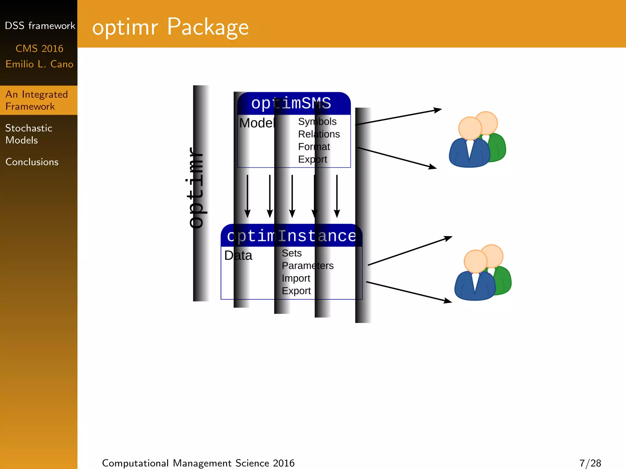
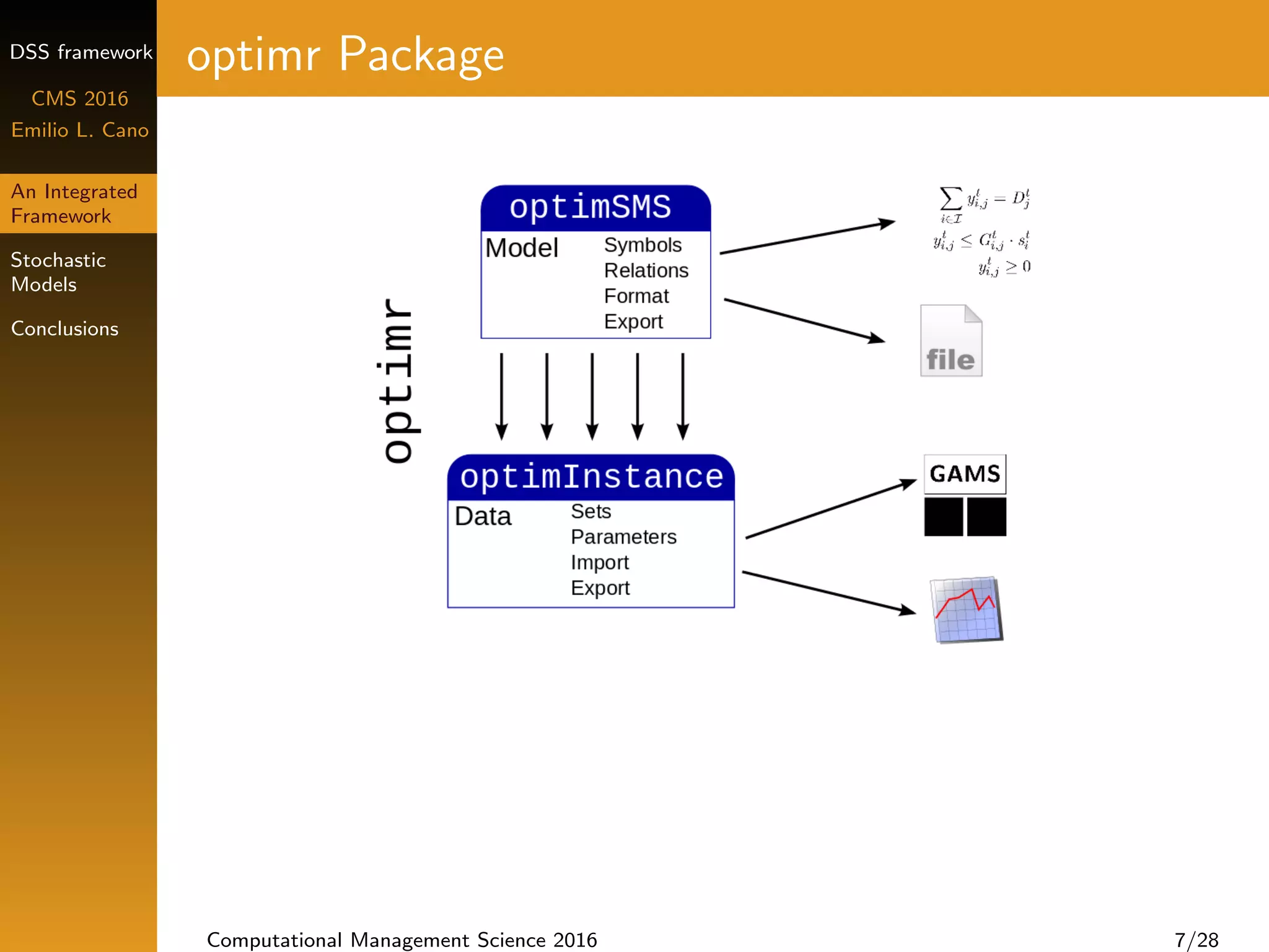
optimr Package
getEq(model1SMS, 4, format = "gams")
## [1] "eqDemand(j,t) ..nt Sum((i), y(i,j,t)) =e= D(j,t) n;n"
Computational Management Science 2016 7/28](https://image.slidesharecdn.com/elcanocms2016slides-160805093244/75/Energy-efficient-technology-investments-using-a-decision-support-system-framework-15-2048.jpg)
![DSS framework
CMS 2016
Emilio L. Cano
An Integrated
Framework
Stochastic
Models
Conclusions
comprehensiveExample.Rnw
documentclass [ a4paper ]{ a r t i c l e }
usepackage {Sweave}
t i t l e { Comprehensive Example f o r
``An I n t e g r a t e d Framework f o r the
R e p r e s e n t a t i o n and S o l u t i o n of S t o c h a s t i c
Energy Optimization Problems ' '}
author { Emilio L . Cano}
<<i n t r o , echo=FALSE , r e s u l t s=hide>>=
## System r e q u i r e m e n t s
## − The R s o f t w a r e and the packages loaded below
## − A l i c e n c e d GAMS i n s t a l l a t i o n . I f GAMS d i r e c t o r y
## i s other than ”˜/ app/gams23 . 9 ” , change the l i n e
## ' igdx (”˜/ app/gams23 . 9 ”) '
## − A LaTeX d i s t r i b u t i o n f o r the c u r r e n t system
## Load needed packages
l i b r a r y ( k n i t r )
l i b r a r y ( optimr )
l i b r a r y ( gdxrrw )
l i b r a r y ( x t a b l e )
l i b r a r y ( ggplot2 )
l i b r a r y ( g r i d )
## T e l l gdxrrw where GAMS i s i n s t a l l e d
igdx (”˜/ app/gams23 . 9 ”)
## Run s c r i p t s with data
## D e t e r m i n i s t i c model
Computational Management Science 2016 10/28](https://image.slidesharecdn.com/elcanocms2016slides-160805093244/75/Energy-efficient-technology-investments-using-a-decision-support-system-framework-19-2048.jpg)
![DSS framework
CMS 2016
Emilio L. Cano
An Integrated
Framework
Stochastic
Models
Conclusions
comprehensiveExample.Rnw (cont.)
source ( ”. / data /model1SMS .R ”)
## S t o c h a s t i c e x t e n s i o n
source ( ”. / data /model2SMS .R ”)
## I n s t a n c e with 100 s c e n a r i o s
source ( ”. / data / model2Instance2 .R ”)
@
begin {document}
SweaveOpts{ concordance=TRUE}
m a k e t i t l e
s e c t i o n { I n t r o d u c t i o n }
This document i s an example on how to use t e x t s f {R} as an i n t e g r a t e d
environment f o r o p t i m i z a t i o n . I t i s assumed that the t e x t s f { optimr } package i s
Here we can i n c l u d e any s t a t i s t i c a l a n a l y s i s , f o r example a time s e r i e s a n a l y s i s
to f o r e c a s t the f u t u r e energy p r i c e s , s a v i n g the v a l u e s as parameters . We can
a l s o show g r a p h i c a l r e p r e s e n t a t i o n s of the parameter values , as i n Figure ˜ r e f { f
begin { f i g u r e }[ htp ]
begin { c e n t e r }
<<examplepar , f i g=TRUE, echo=FALSE , width=10>>=
## Demand
dtoPlot <− i n s t a n c e P a r s ( model2Instance2 , ”D”)
d t o P l o t $ i d <− 1:20
pD <− ggplot ( data = dtoPlot , aes ( x = id , y = value , group=n , c o l=n ))
pD <− pD + geom path ()
pD <− pD + s c a l e x d i s c r e t e (name = ”” , breaks = seq (1 ,21 , by =5) , l a b e l s = 2013:2
pD <− pD + g g t i t l e ( ”Energy demand ”)
Computational Management Science 2016 11/28](https://image.slidesharecdn.com/elcanocms2016slides-160805093244/75/Energy-efficient-technology-investments-using-a-decision-support-system-framework-20-2048.jpg)
![DSS framework
CMS 2016
Emilio L. Cano
An Integrated
Framework
Stochastic
Models
Conclusions
comprehensiveExample.Rnw (cont.)
}
@
We can embed c a l c u l a t i o n s w i t h i n the text , f o r example the v a l u e of the
o b j e c t i v e f u n c t i o n ( Sexpr { round ( m o d e l 2 I n s t a n c e 2 @ r e s u l t $ o b j )}) , or we can p r i n t
LaTeX˜ t a b l e s with the optimal values , as the ones i n Tables r e f { tab : x} and r e
other a n a l y s i s and r e p r e s e n t a t i o n ( see Figure ˜ r e f { f i g : r e s } ) . See the t e x t t t {.R
<<r e s u l t s=tex , echo=FALSE>>=
p r i n t ( x t a b l e ( i n s t a n c e V a r s ( model2Instance2 , ”x ”) ,
”Optimal v a l u e s f o r $x$ ”,
”tab : x ”) , i n c l u d e . rownames = FALSE)
p r i n t ( x t a b l e ( head ( i n s t a n c e V a r s ( model2Instance2 , ”y ”) ) ,
”Optimal v a l u e s f o r $y$ ( f i r s t 6 v a l u e s ) ”,
”tab : y ”) , i n c l u d e . rownames = FALSE)
@
begin { f i g u r e }[ htp ]
begin { c e n t e r }
<<bar , echo=FALSE , f i g=TRUE>>=
d f 2 p l o t <− s ub s e t ( i n s t a n c e V a r s ( model2Instance2 , ”y ”) , j == ”autumn ”)
d f 2 p l o t <− aggregate ( v a l u e ˜ i + t , data = df2plot , FUN = mean)
d f 2 p l o t $ t <− as . i n t e g e r ( as . c h a r a c t e r ( d f 2 p l o t $ t ))
p <− ggplot ( df2plot , aes ( x=t ))
p <− p + geom area ( aes ( y=value , f i l l =i ))
p <− p + l a b s ( t i t l e = ”Optimal production p l a n s (Autumn ) ”, x = ”Year ”, y = ”kW”)
p <− p + s c a l e f i l l d i s c r e t e ( ”Technology ”)
p r i n t ( p )
@
Computational Management Science 2016 15/28](https://image.slidesharecdn.com/elcanocms2016slides-160805093244/75/Energy-efficient-technology-investments-using-a-decision-support-system-framework-24-2048.jpg)
![DSS framework
CMS 2016
Emilio L. Cano
An Integrated
Framework
Stochastic
Models
Conclusions
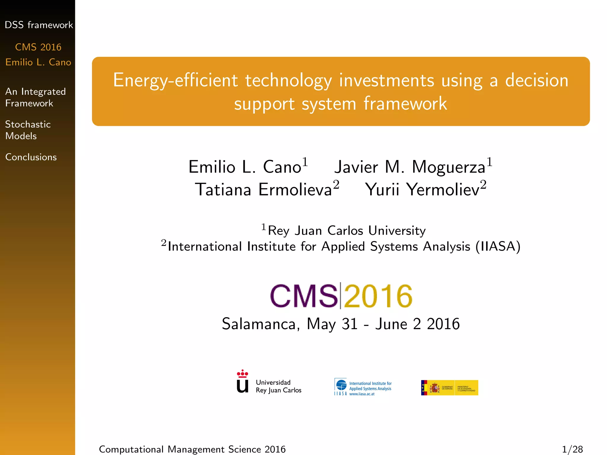
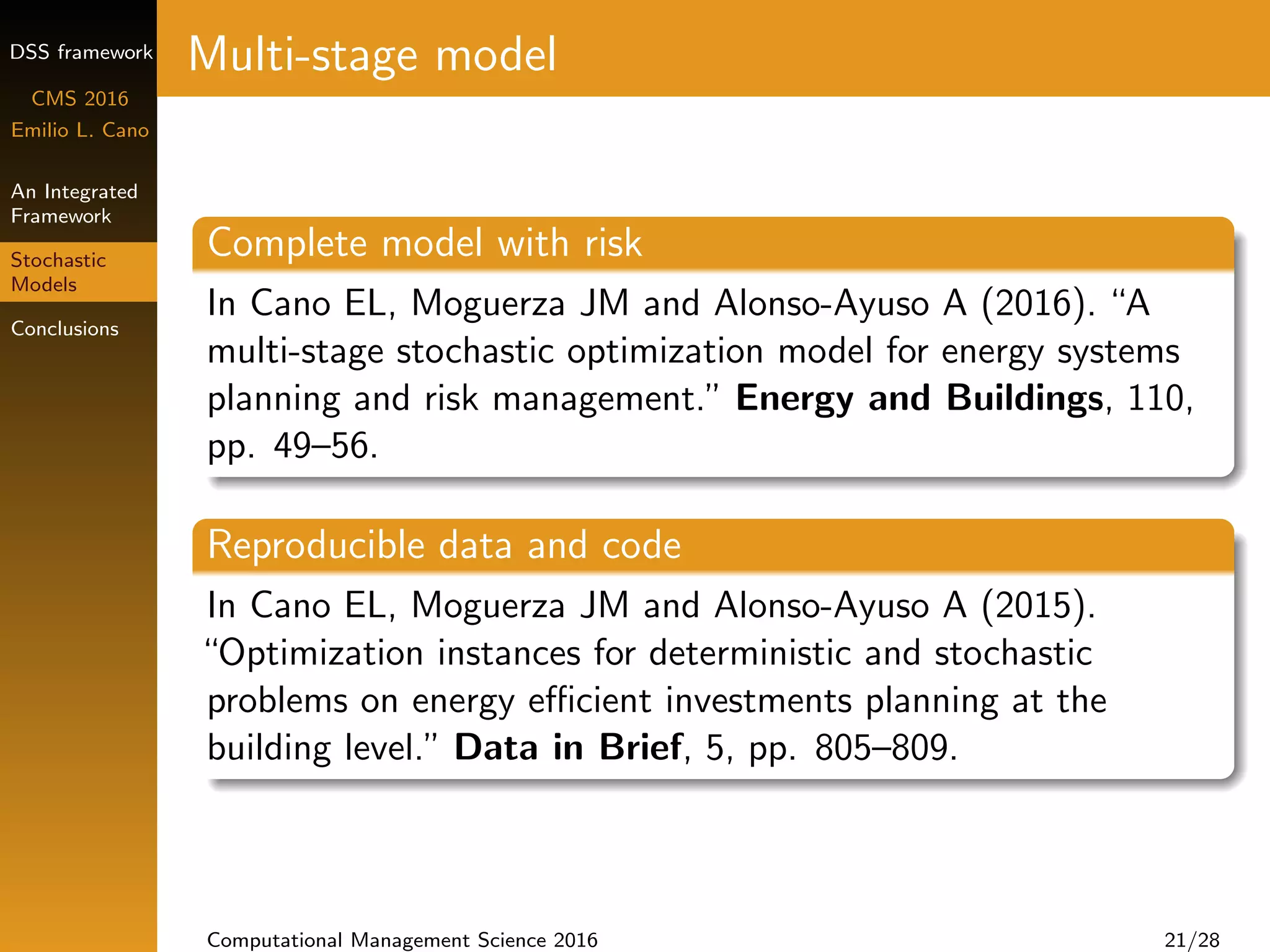
Multi-stage model with risk management
Different objectives: min cost, emissions, or energy use
Risk measure CVaR [Rockafellar and Uryasev (2000)]
Weighted objective function
Computational Management Science 2016 22/28](https://image.slidesharecdn.com/elcanocms2016slides-160805093244/75/Energy-efficient-technology-investments-using-a-decision-support-system-framework-36-2048.jpg)

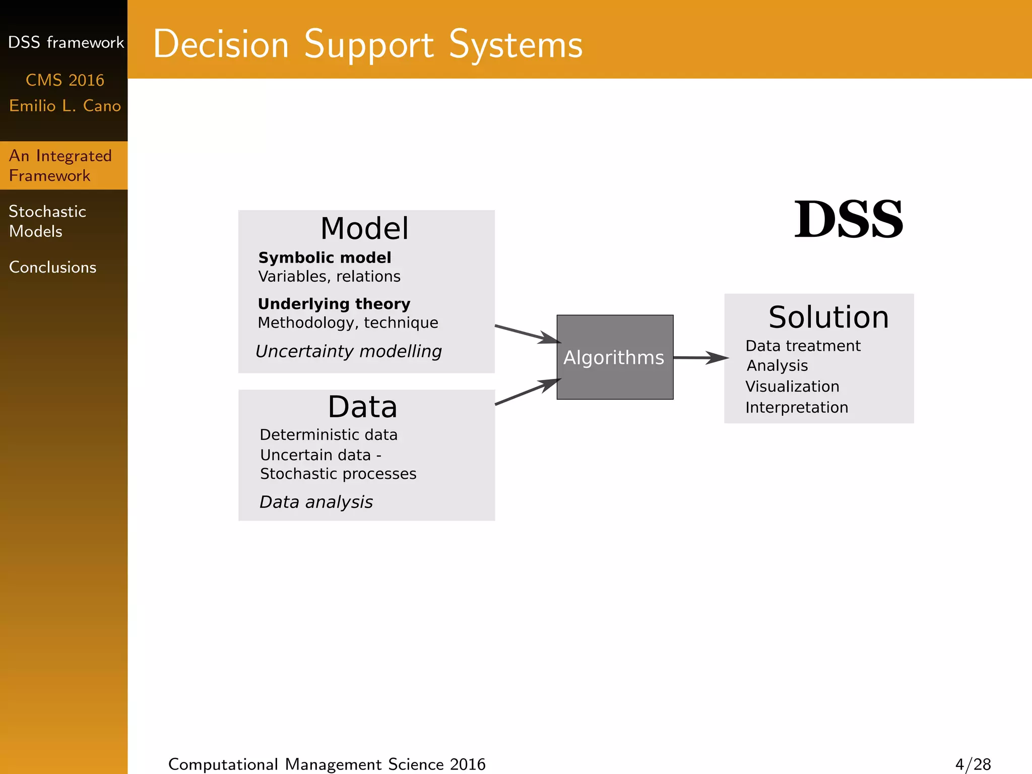
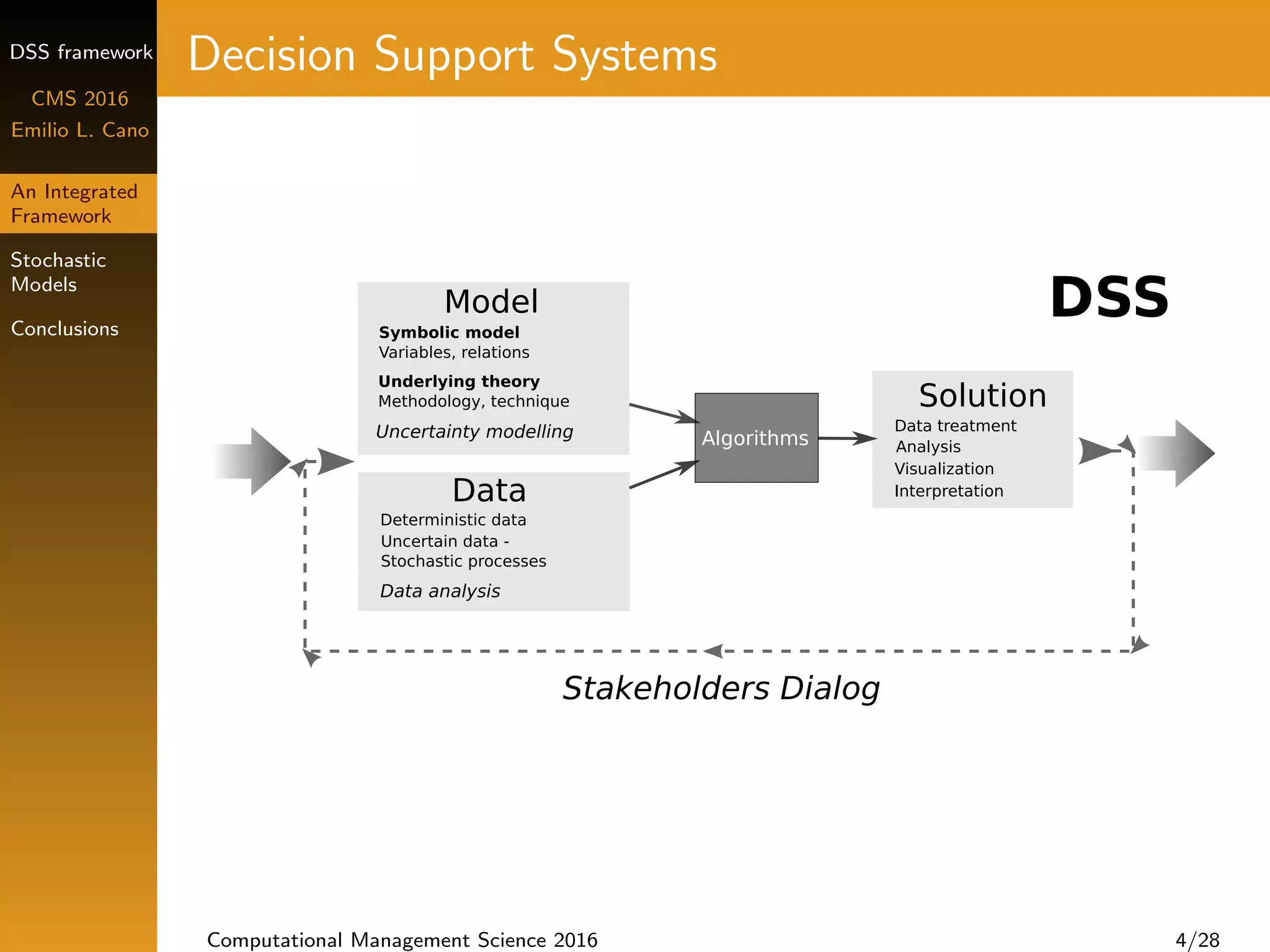
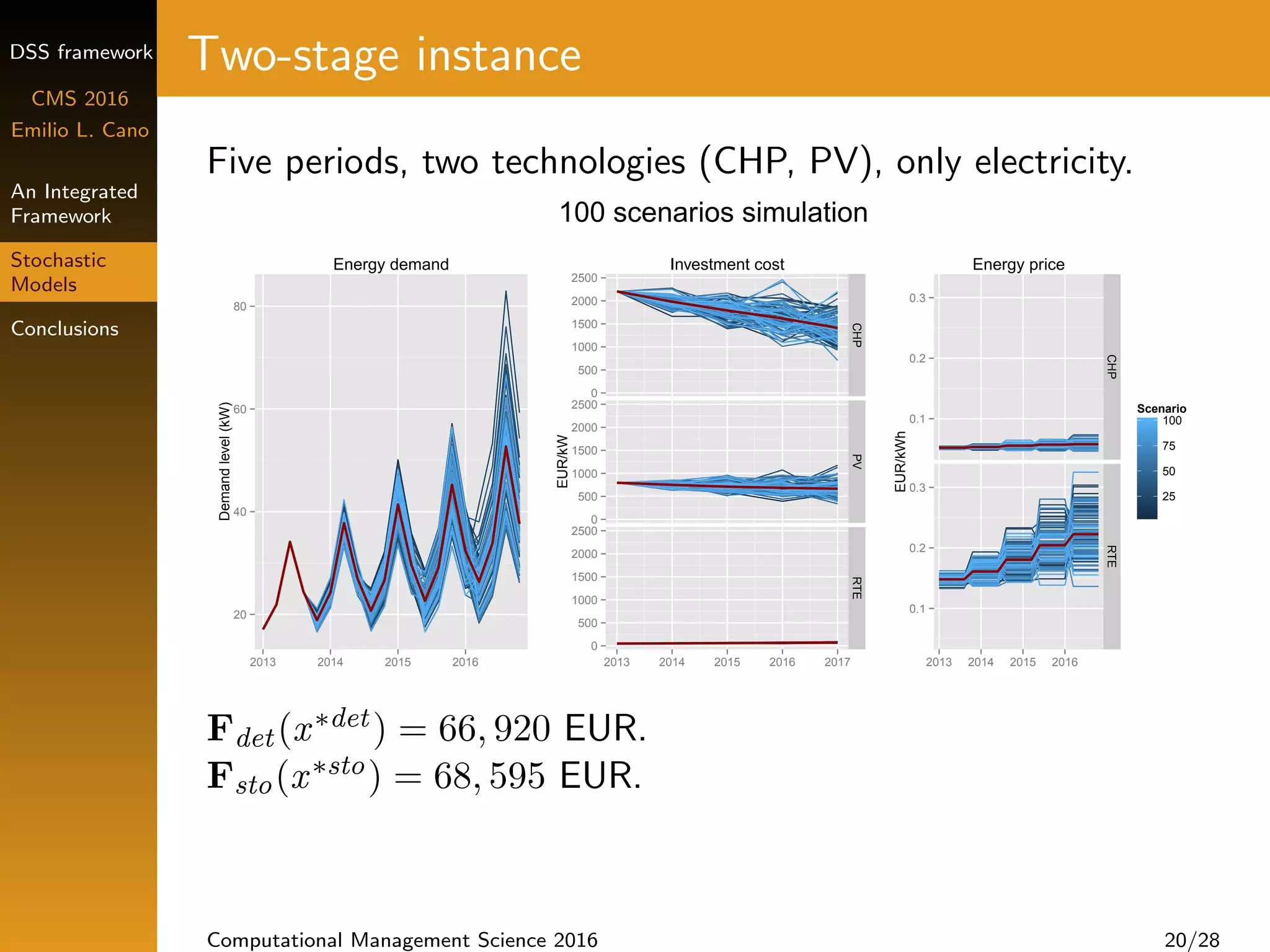
This document presents an integrated framework for decision support systems using R. It describes using R and related packages to represent stochastic energy optimization problems, generate input files for solvers, analyze results, and produce reproducible reports. Stochastic models are developed and solved within this framework. The framework allows statistical analysis, graphical output, model equations, solver inputs/outputs, and comprehensive reports to be combined for modeling, analysis, and stakeholder communication.