Download as PDF, PPTX
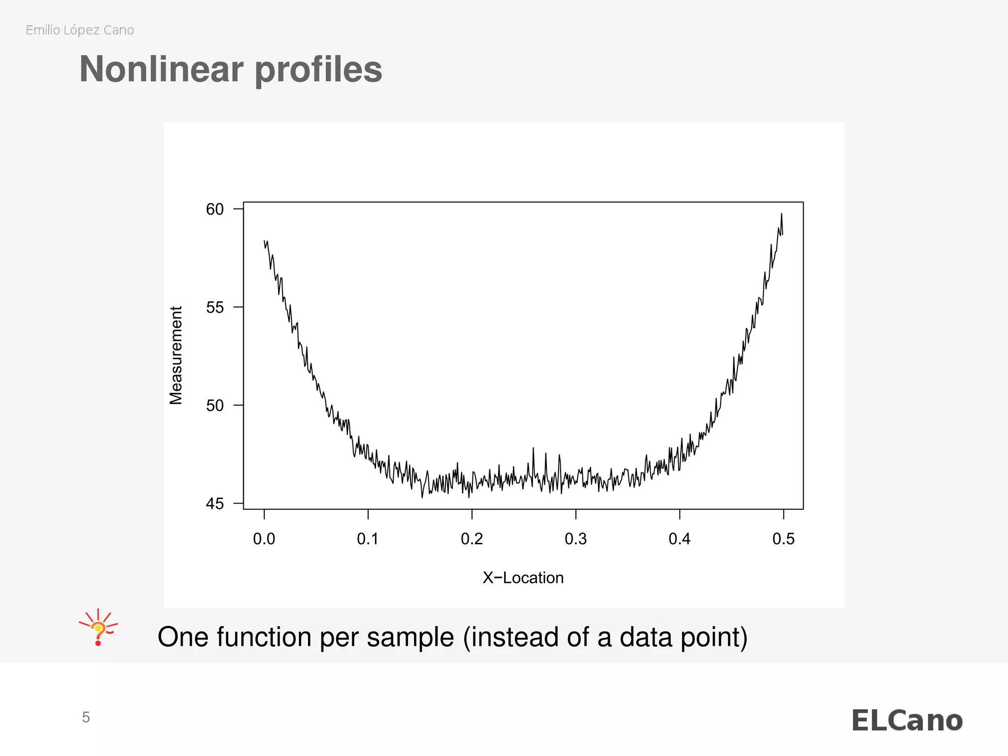
![Illustrative example (cont.)
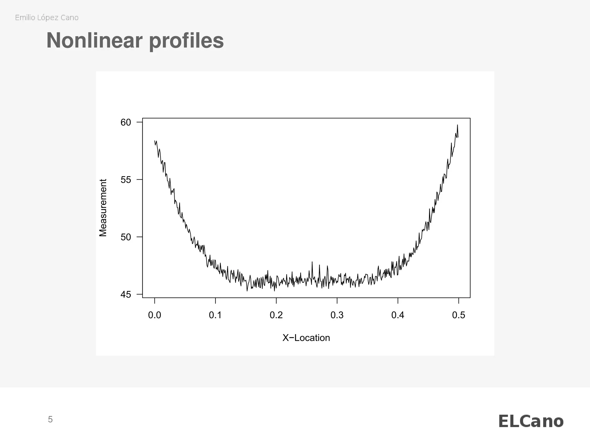
Data
library(SixSigma)
str(ss.data.wbx)
## num [1:500] 0 0.001 0.002 0.003 0.004 0.005 0.006 0.007
str(ss.data.wby)
## num [1:500, 1:50] 58.4 58 58.2 58.4 57.9 ...
## - attr(*, "dimnames")=List of 2
## ..$ : NULL
## ..$ : chr [1:50] "P1" "P2" "P3" "P4" ...
7](https://image.slidesharecdn.com/02presentation-170825200202/75/Unattended-SVM-parameters-fitting-for-monitoring-nonlinear-profiles-8-2048.jpg)
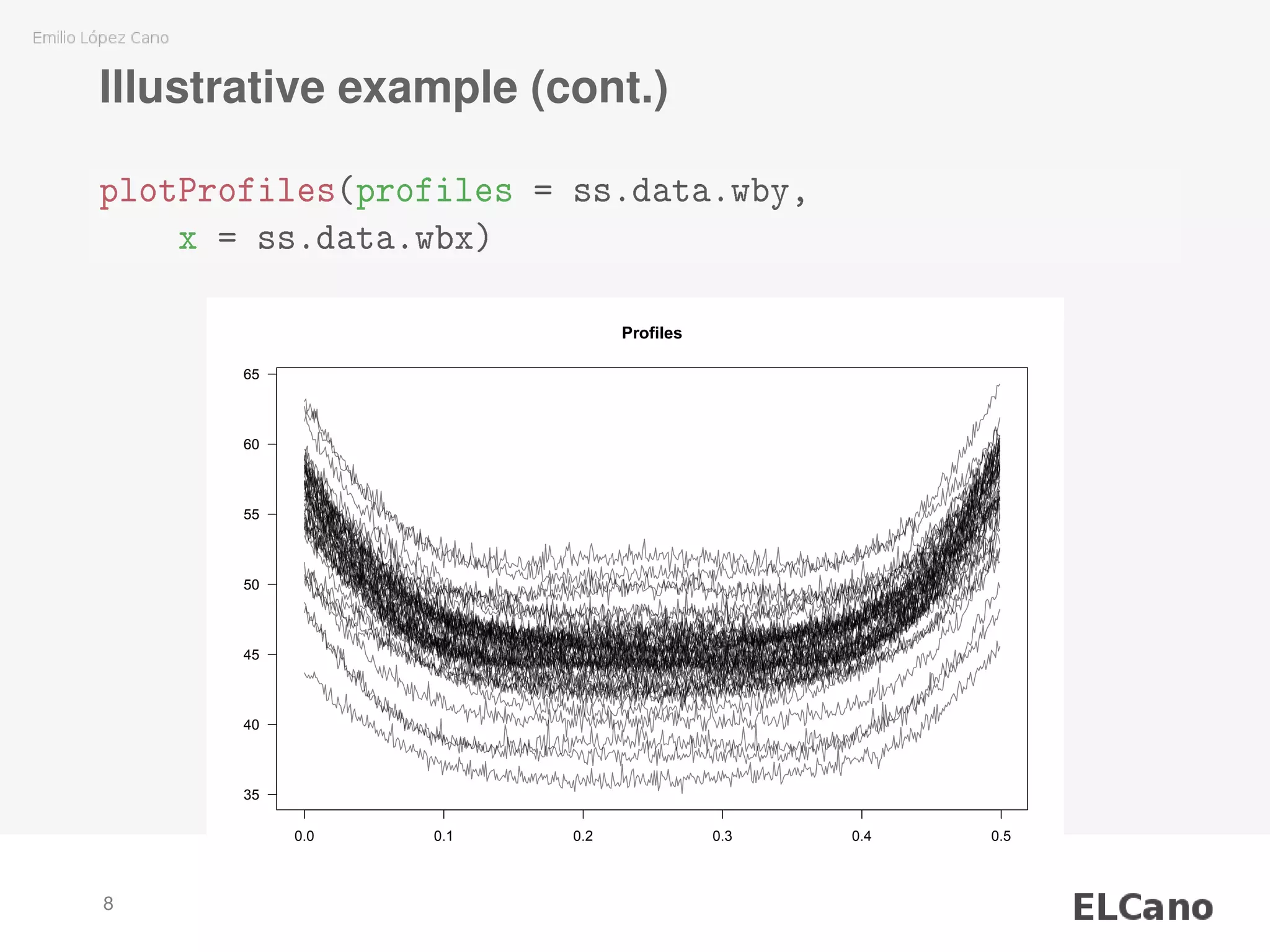
![Regularization of nonlinear profiles via SVM
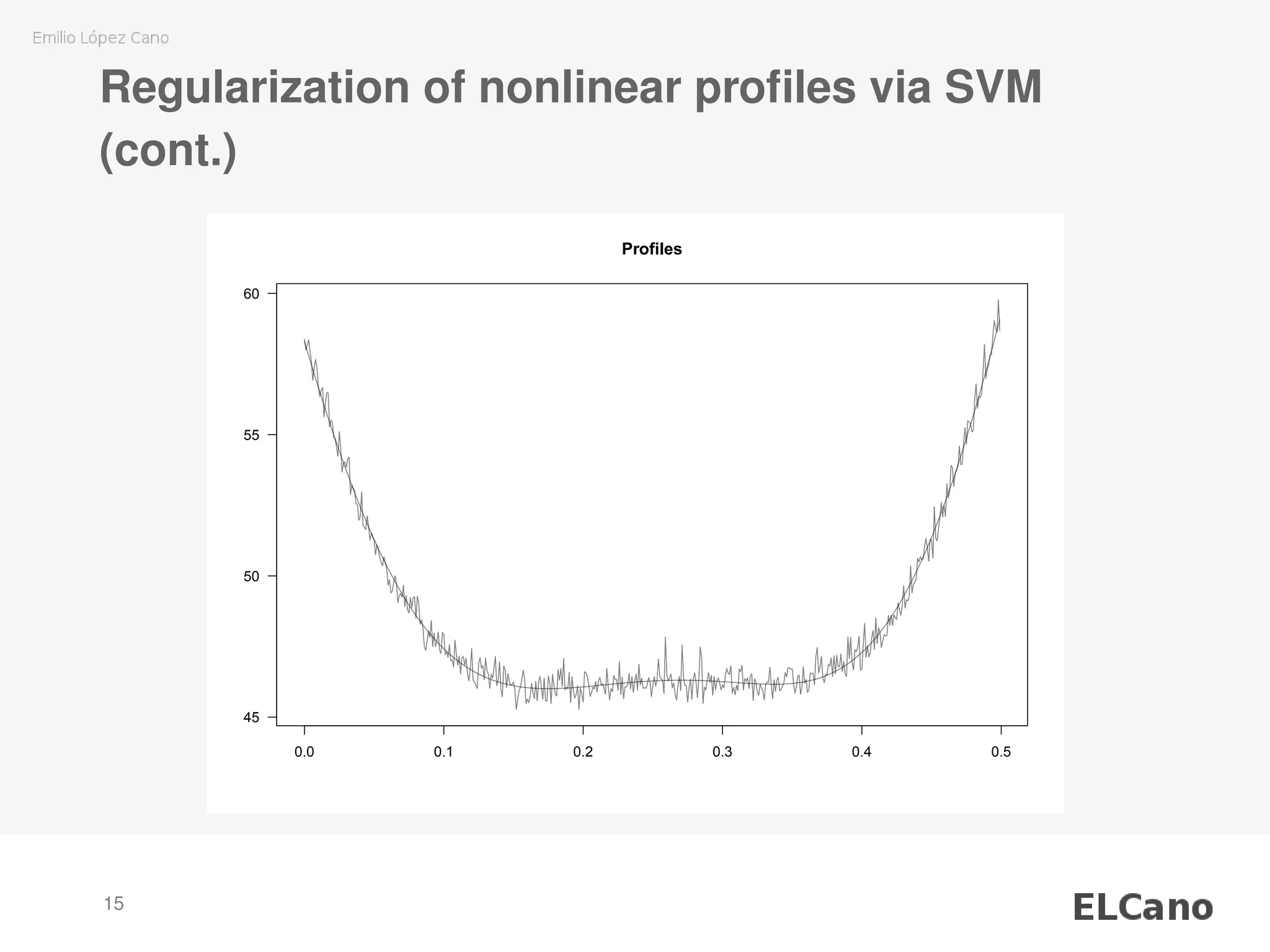
P1.smooth <- smoothProfiles(
profiles = ss.data.wby[, "P1"],
x = ss.data.wbx)
plotProfiles(profiles = cbind(P1.smooth,
ss.data.wby[, "P1"]),
x = ss.data.wbx)
14](https://image.slidesharecdn.com/02presentation-170825200202/75/Unattended-SVM-parameters-fitting-for-monitoring-nonlinear-profiles-15-2048.jpg)
![Smoothed prototype and confidence bands
(cont.)
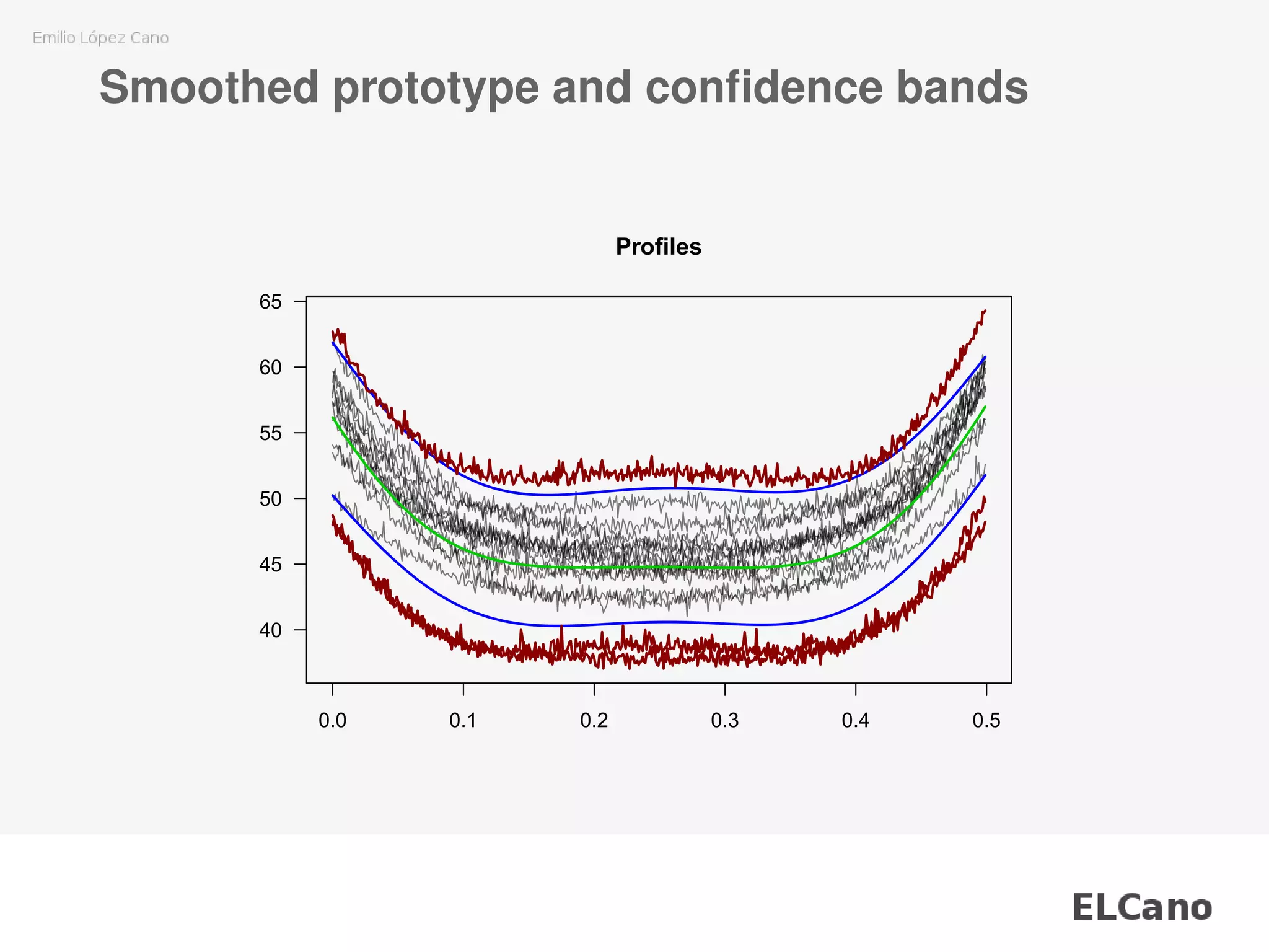
wby.phase1 <- ss.data.wby[, 1:35]
wb.limits <- climProfiles(profiles = wby.phase1[, -28],
x = ss.data.wbx,
smoothprof = TRUE,
smoothlim = TRUE)
wby.phase2 <- ss.data.wby[, 36:50]
wb.out.phase2 <- outProfiles(profiles = wby.phase2,
x = ss.data.wbx,
cLimits = wb.limits,
tol = 0.8)
plotProfiles(wby.phase2,
x = ss.data.wbx,
cLimits = wb.limits,
outControl = wb.out.phase2$idOut,
onlyout = FALSE)](https://image.slidesharecdn.com/02presentation-170825200202/75/Unattended-SVM-parameters-fitting-for-monitoring-nonlinear-profiles-18-2048.jpg)


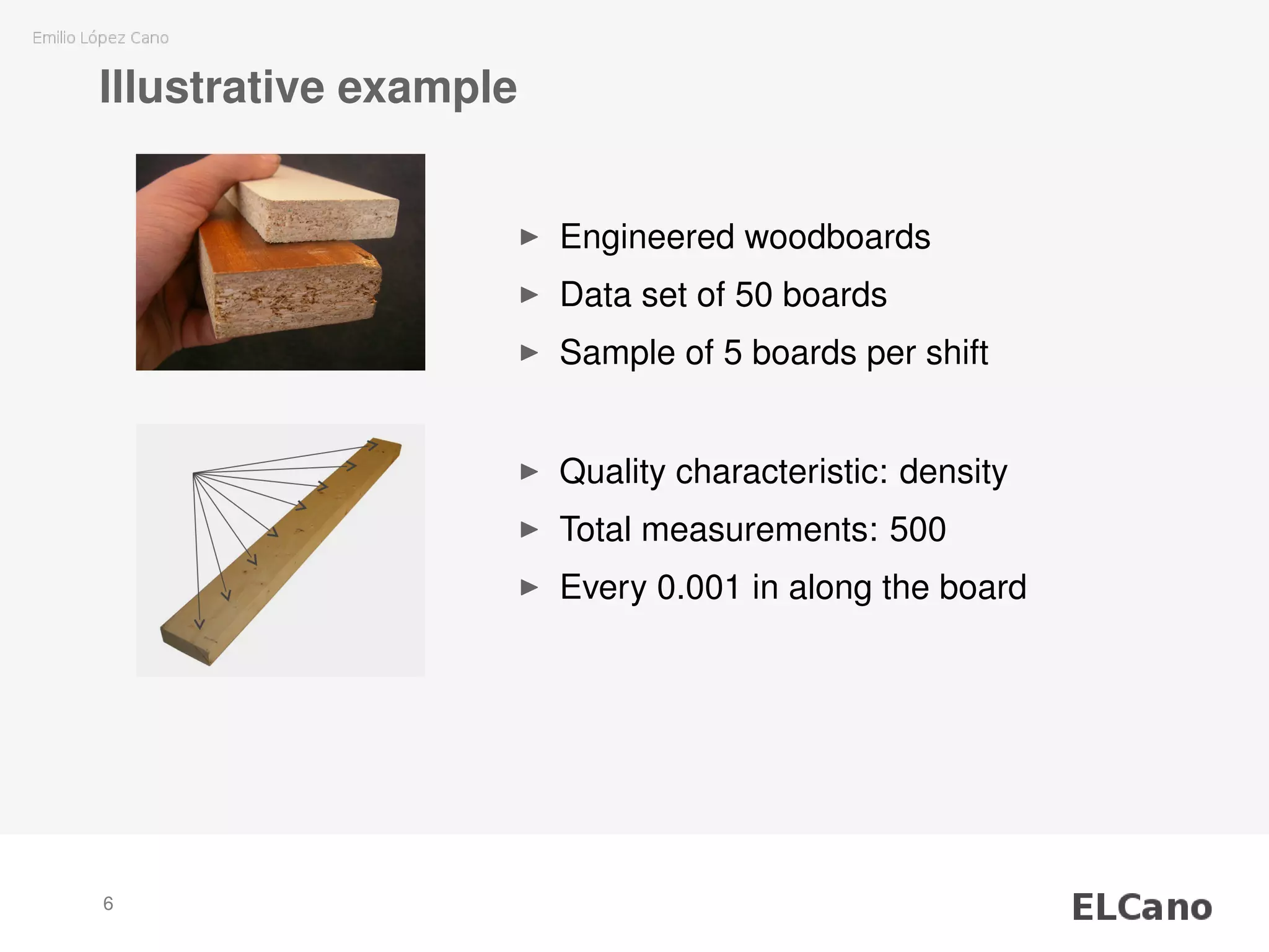
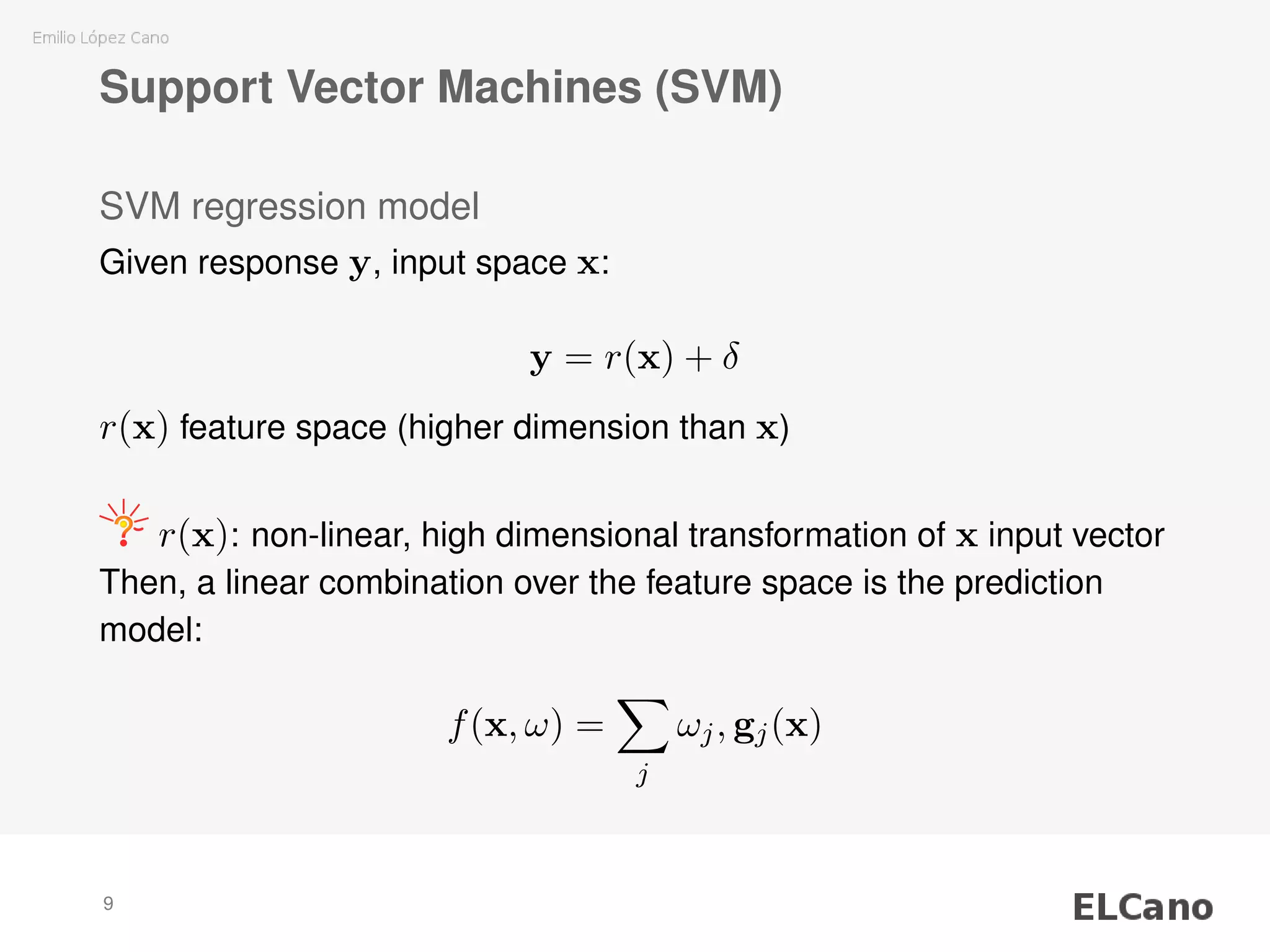
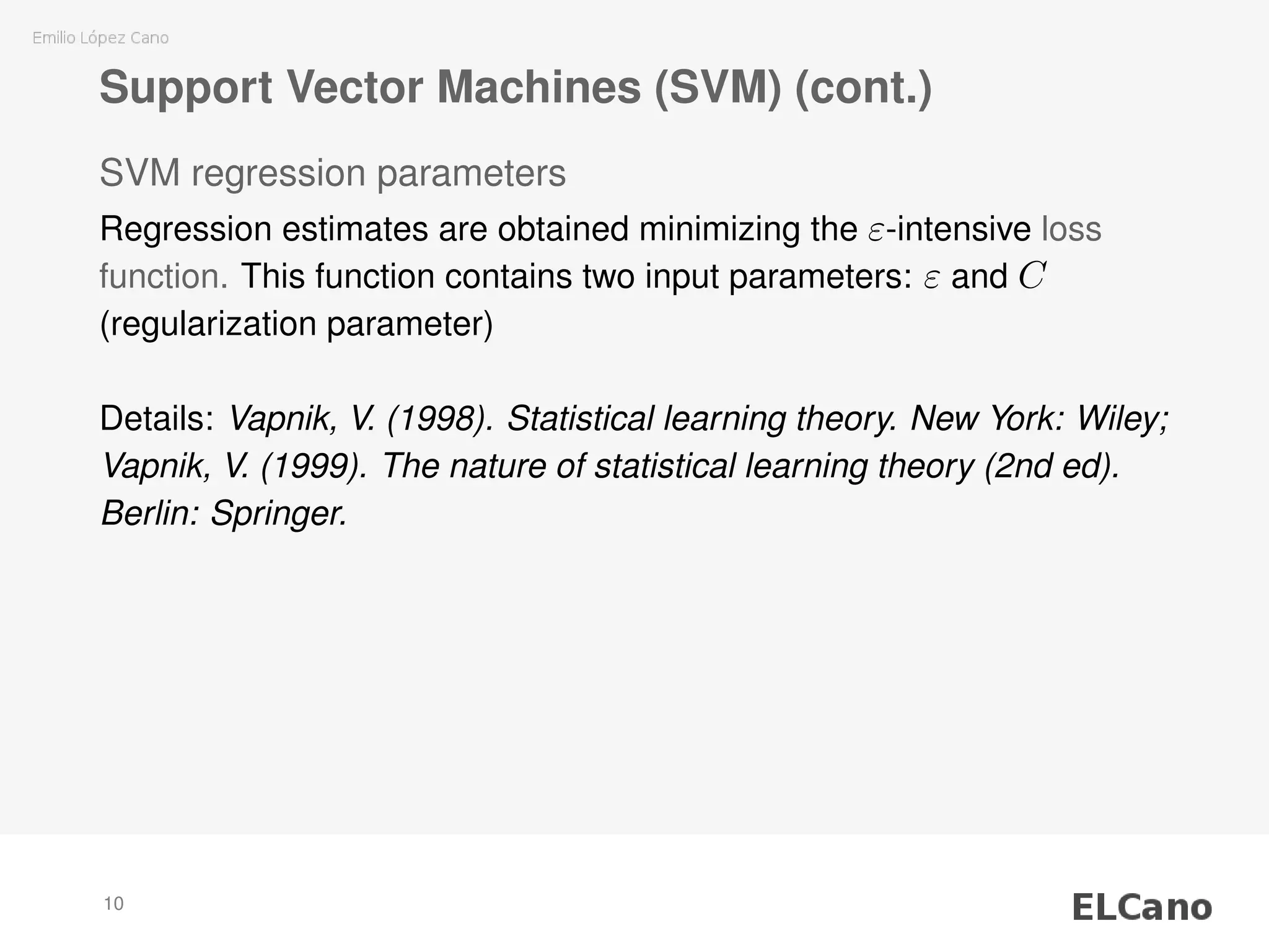
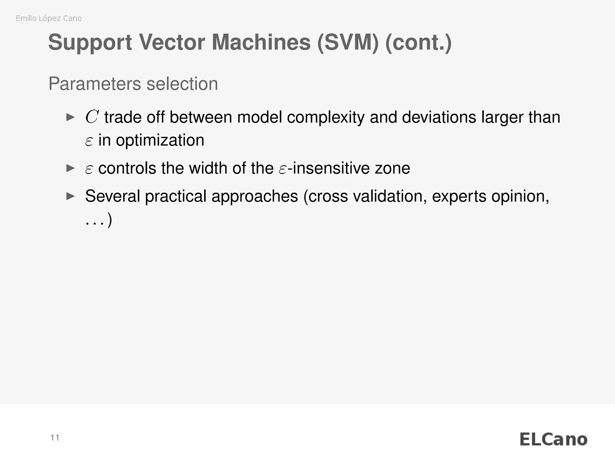
This document discusses using support vector machines (SVM) for unattended parameter fitting to monitor nonlinear profiles. It presents an illustrative example of using SVM regression to smooth measured density profiles of engineered wood boards. The key points are: 1) SVM regression requires selecting parameters C (regularization parameter) and ε (width of insensitive zone), which control the complexity and deviations of the model. 2) Methods are presented for unattended selection of C and ε based on properties of the input noise and data. 3) The SVM model is applied to smooth individual nonlinear profiles from measured wood board density data and identify potential outliers.


![SVM[Support vector Machine] Machine learning](https://cdn.slidesharecdn.com/ss_thumbnails/svm-250403184638-1cd9afdb-thumbnail.jpg?width=640&height=640&fit=bounds)


