Download to read offline


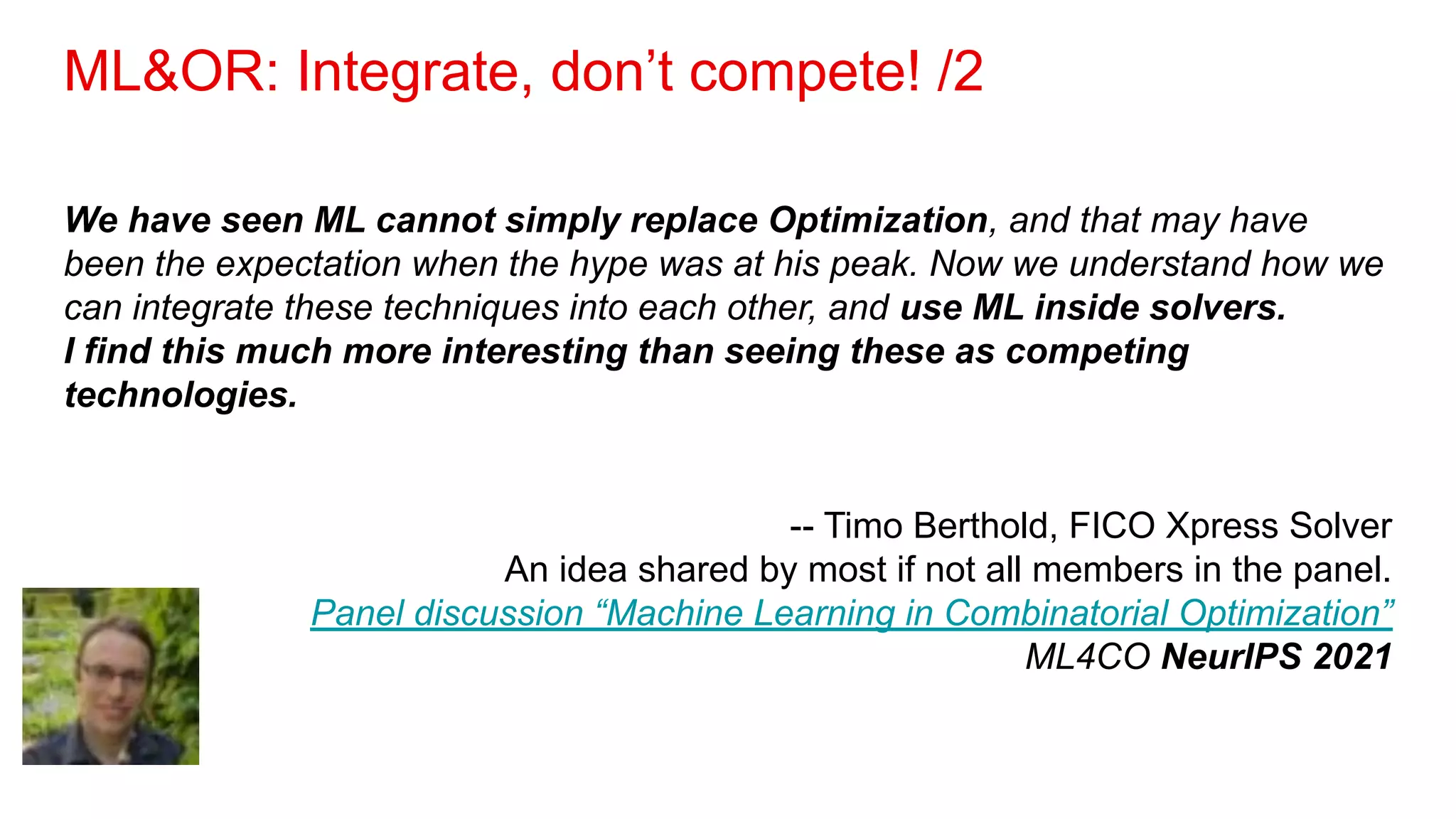
![ML&OR: Integrate, don’t compete! /1
Is combinatorial optimization the right domain for ML? Classical solvers are
extremely mature and very powerful. It is not clear there’s a huge improvement by
applying ML, whereas there could be other domains [in combinatorial
optimization] where ML could shine brighter.
-- Vinod Nair, DeepMind
Panel discussion “Machine Learning in Combinatorial Optimization”
ML4CO NeurIPS 2021](https://image.slidesharecdn.com/atavernadli2022-220720193352-c7307200/75/Meetup-Luglio-Operations-Research-pdf-25-2048.jpg)


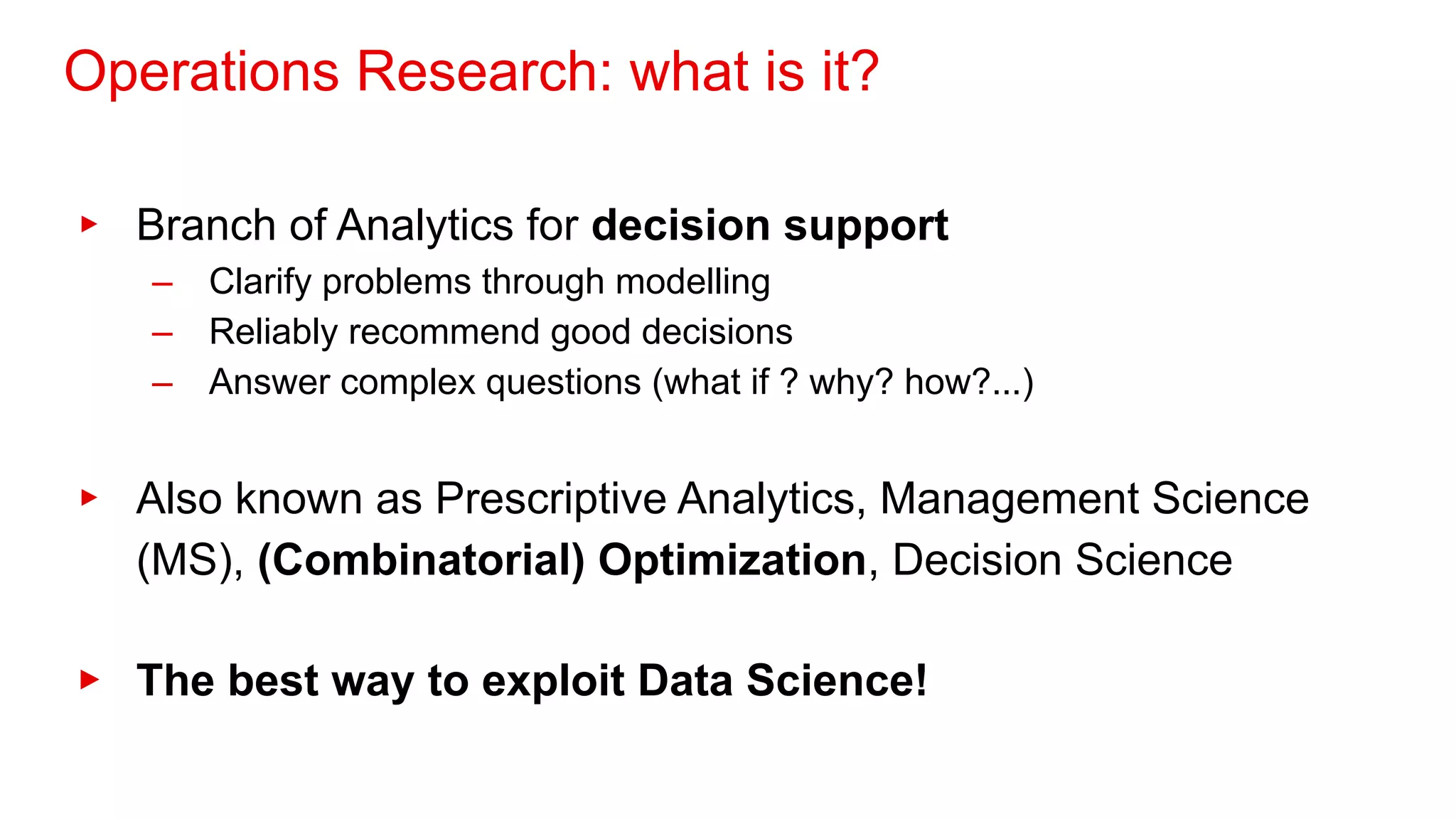
1. The document discusses operations research, which uses mathematical modeling to help make better decisions. 2. Operations research tools like mathematical programming and decomposition methods can be used to solve large, complex problems and scale to practical applications. 3. Decomposition methods break large problems into smaller subproblems that can be solved independently to find good feasible solutions for the original problem.


![[DSC Europe 25] Uros Pesic - The Reality of AI in Marketing.pdf](https://cdn.slidesharecdn.com/ss_thumbnails/rtkodnmtycovsllvzsyn-9-251215095918-b0c6bfe3-thumbnail.jpg?width=640&height=640&fit=bounds)


![[DSC Europe 25] Behzad Hosseini - AI Agents in the Wild: Deploying Models tha...](https://cdn.slidesharecdn.com/ss_thumbnails/3qtejajvsjqrzwfept2c-10-251212103250-7f2b1068-thumbnail.jpg?width=640&height=640&fit=bounds)


![[DSC Europe 25] Miodrag Pesovic & Vladislav Radonjic - Federated Data Archite...](https://cdn.slidesharecdn.com/ss_thumbnails/gsbe3y5it5uhndi4e08e-1-251212103249-f1008e0c-thumbnail.jpg?width=640&height=640&fit=bounds)


![[DSC Europe 25] Dunja Adzic Jovanovic - AI and Cybersecurity: Defending Data ...](https://cdn.slidesharecdn.com/ss_thumbnails/o1zylpbhrtwnixxq2xj8-7-251211083048-185086f6-thumbnail.jpg?width=640&height=640&fit=bounds)
![[DSC Europe 25] Hans Kleinsman - The Compliance Gearbox: How Tax Tech Mediate...](https://cdn.slidesharecdn.com/ss_thumbnails/dxdytie1toel0hr90bjs-2-251212103250-174fdbe7-thumbnail.jpg?width=640&height=640&fit=bounds)

![[DSC Europe 25] Branko Dzakula - From Defense to Attack: How AI Redefines Cyb...](https://cdn.slidesharecdn.com/ss_thumbnails/80bdzdxpr3ky2g0qvyk9-8-251211083048-ce5fc1ee-thumbnail.jpg?width=640&height=640&fit=bounds)

![[DSC Europe 25] Katherine Forrest - AI NOW: Understanding the Velocity of Cha...](https://cdn.slidesharecdn.com/ss_thumbnails/wvvbruqfrci0sfq9xwgb-4-251212104007-e5ad1987-thumbnail.jpg?width=640&height=640&fit=bounds)
