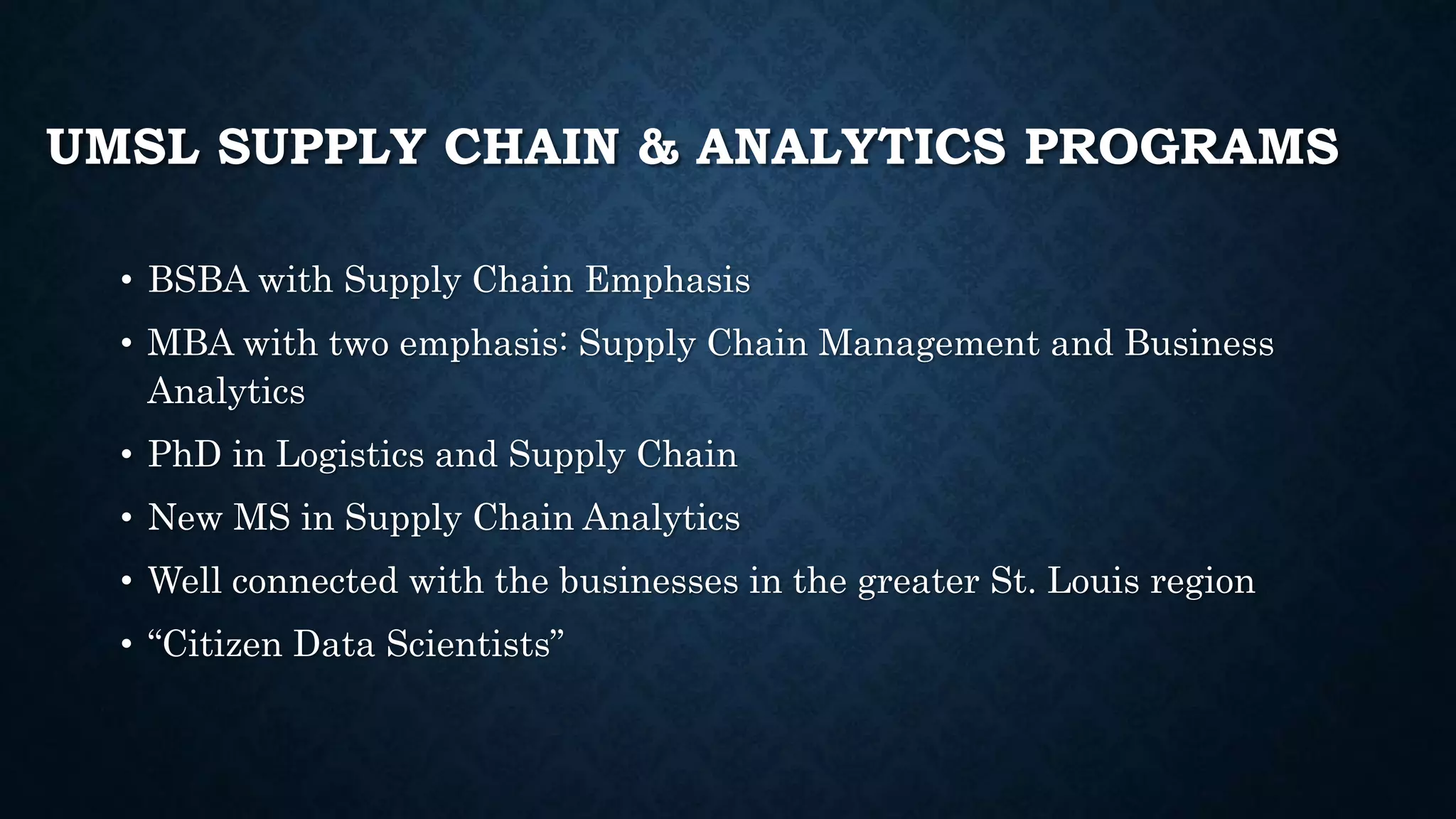
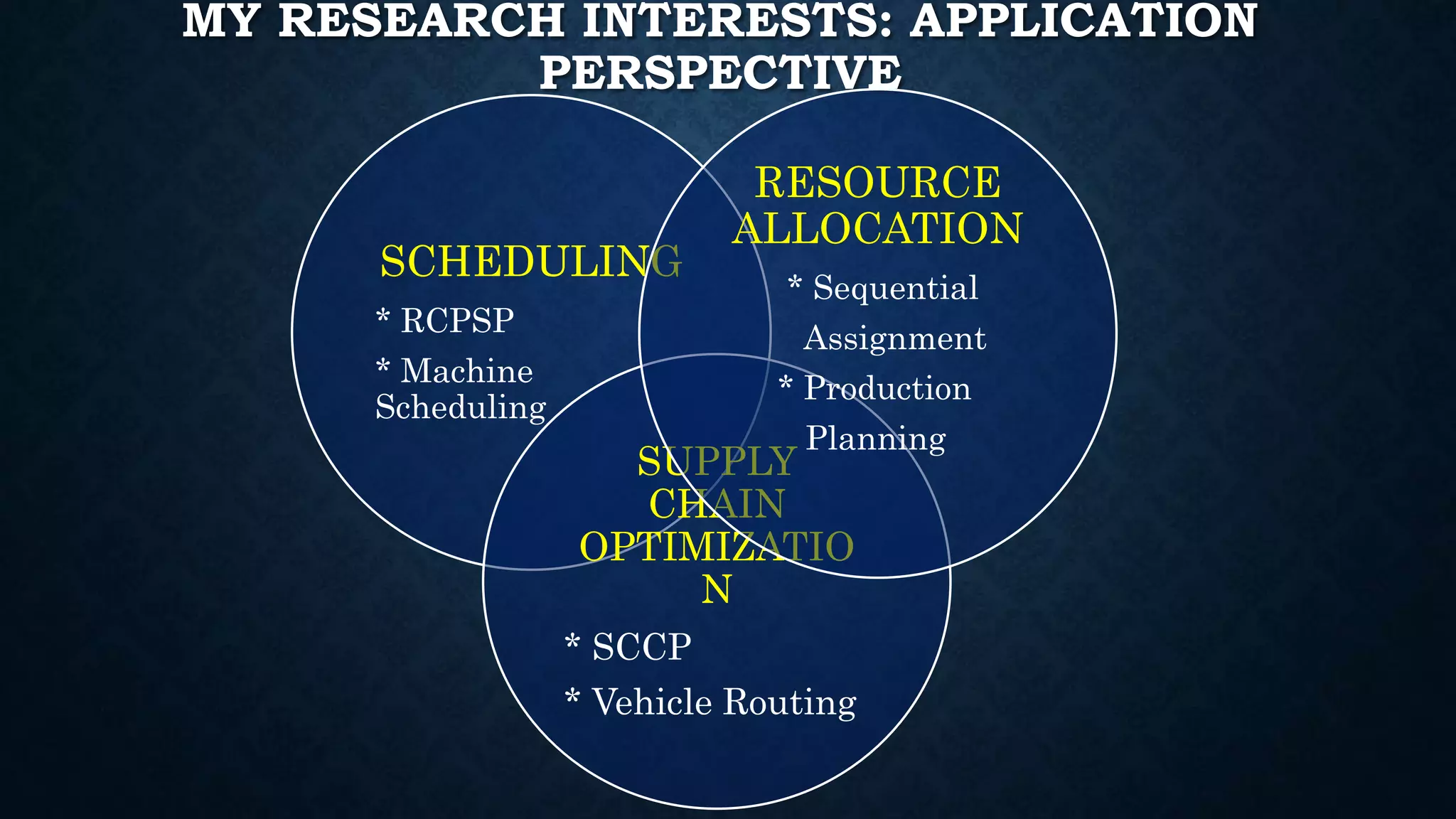
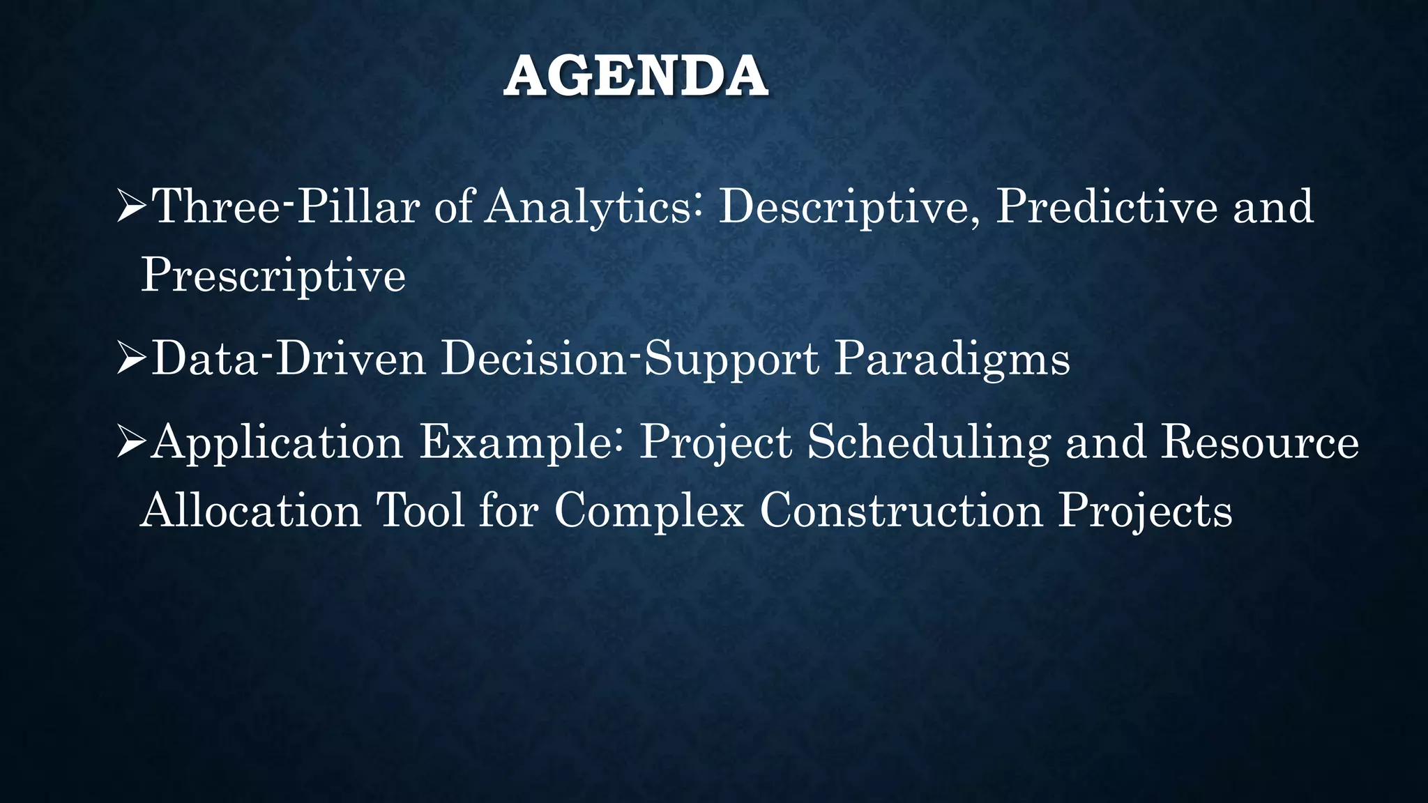
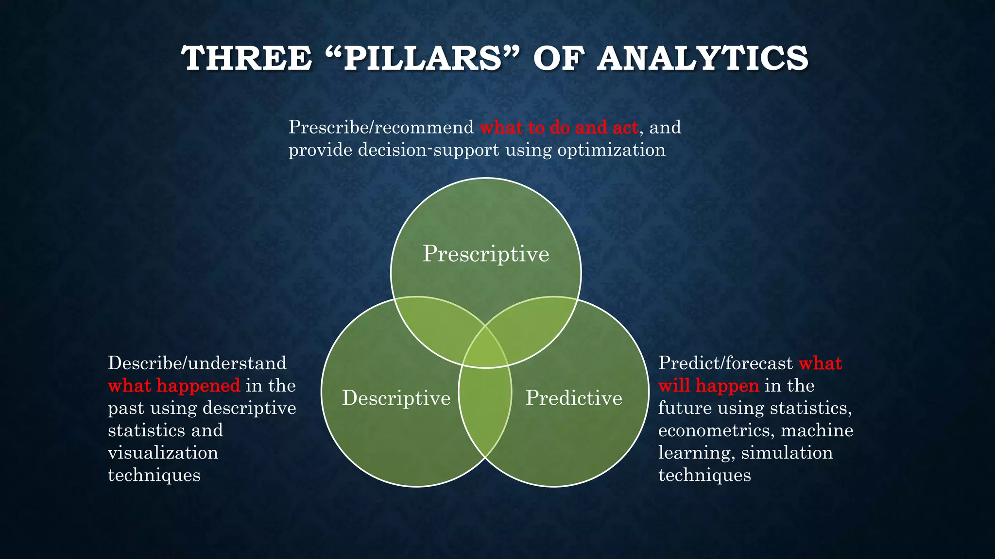
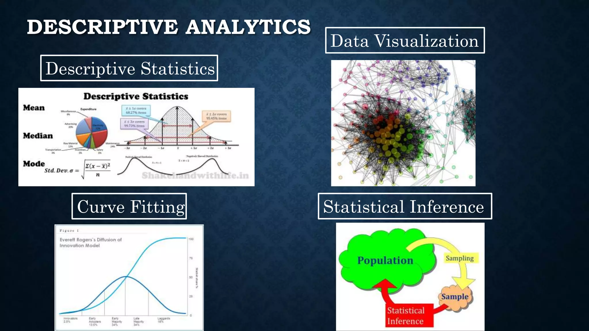
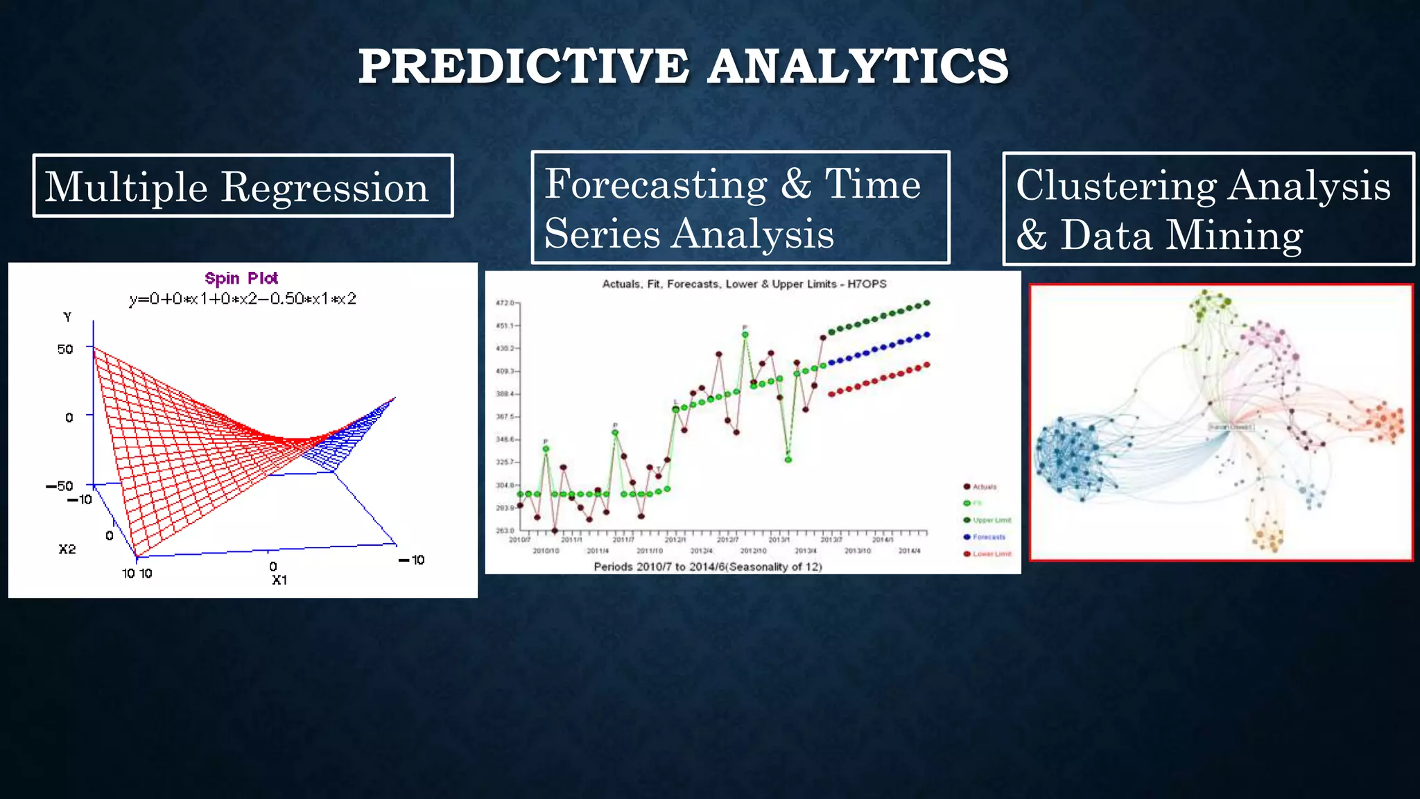
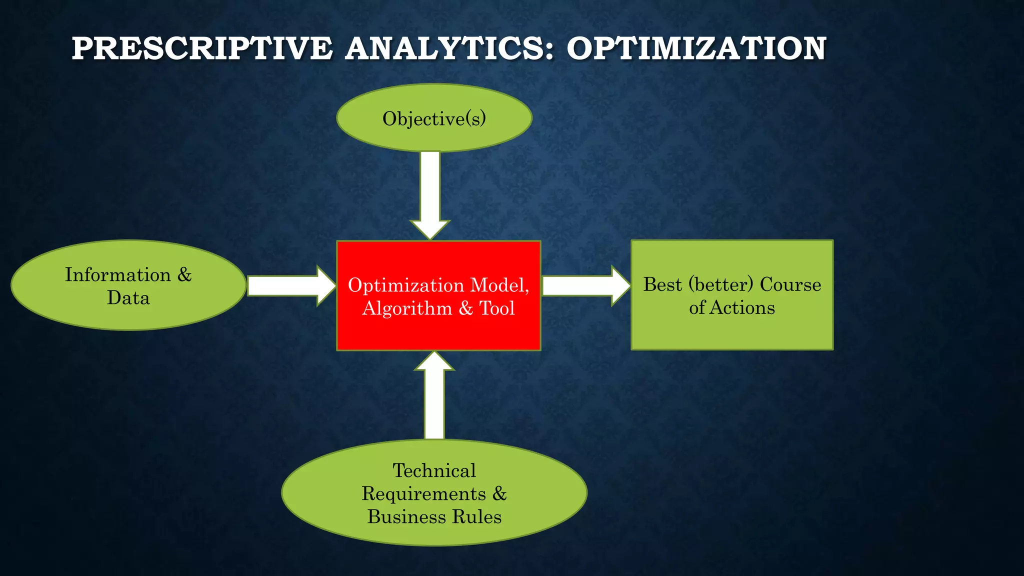
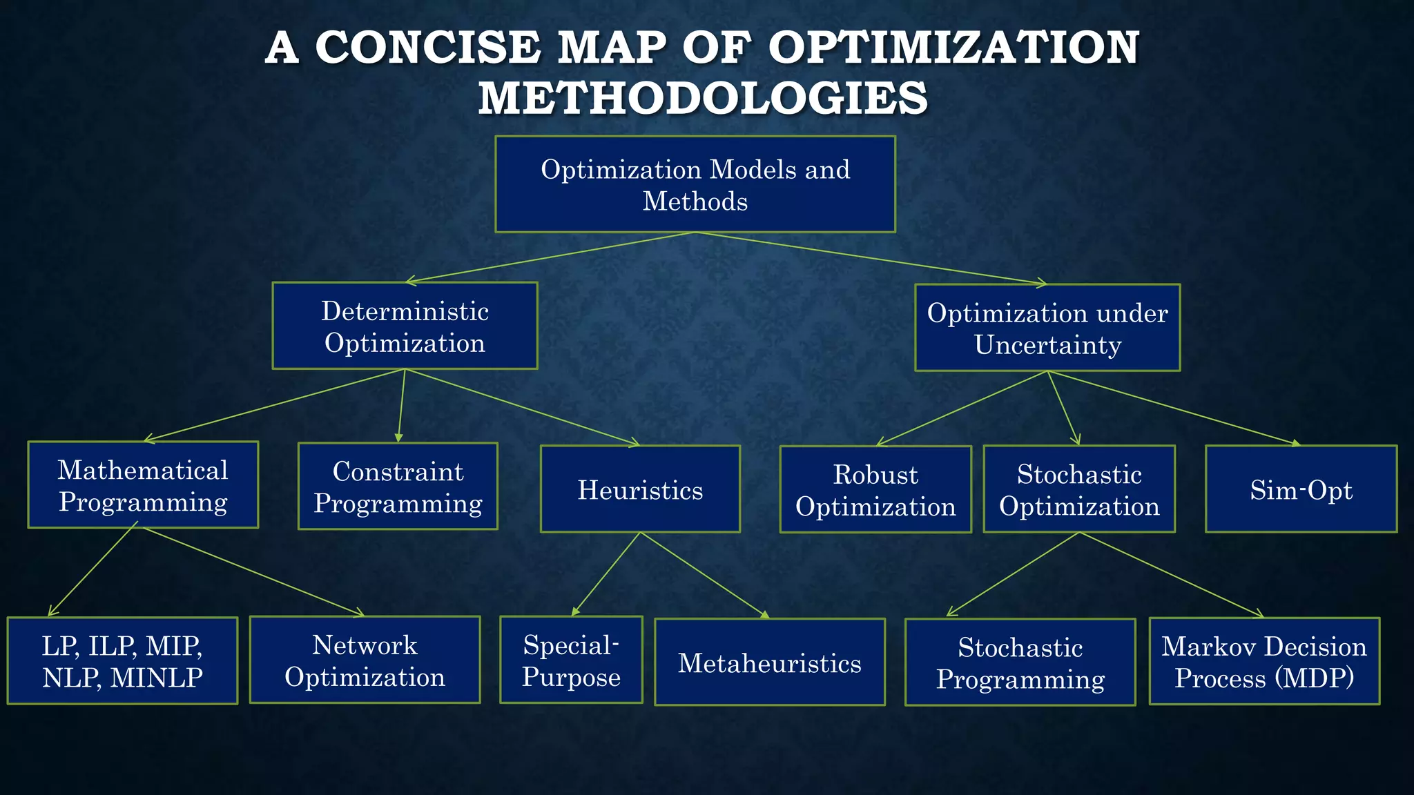
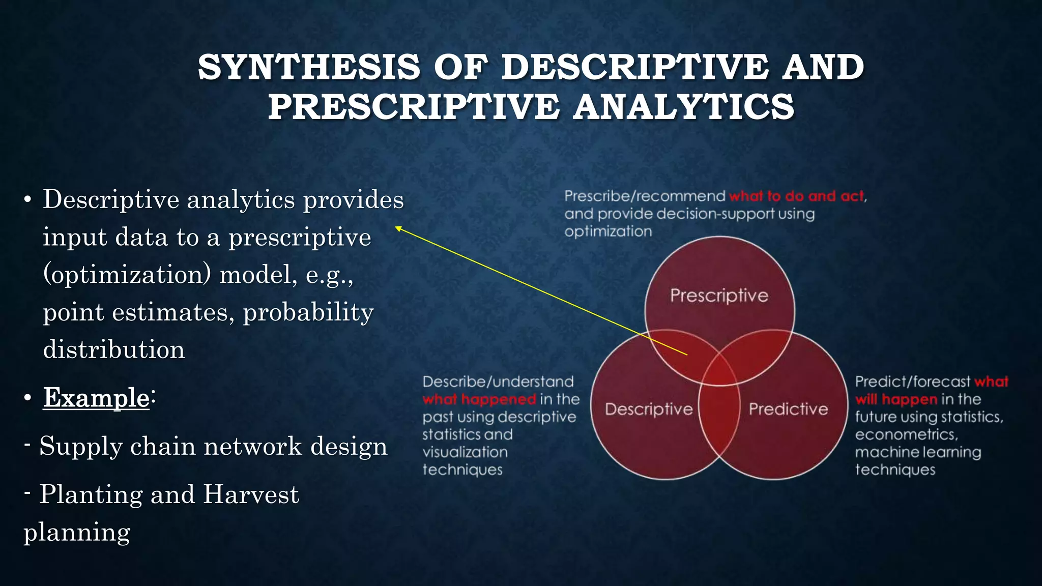
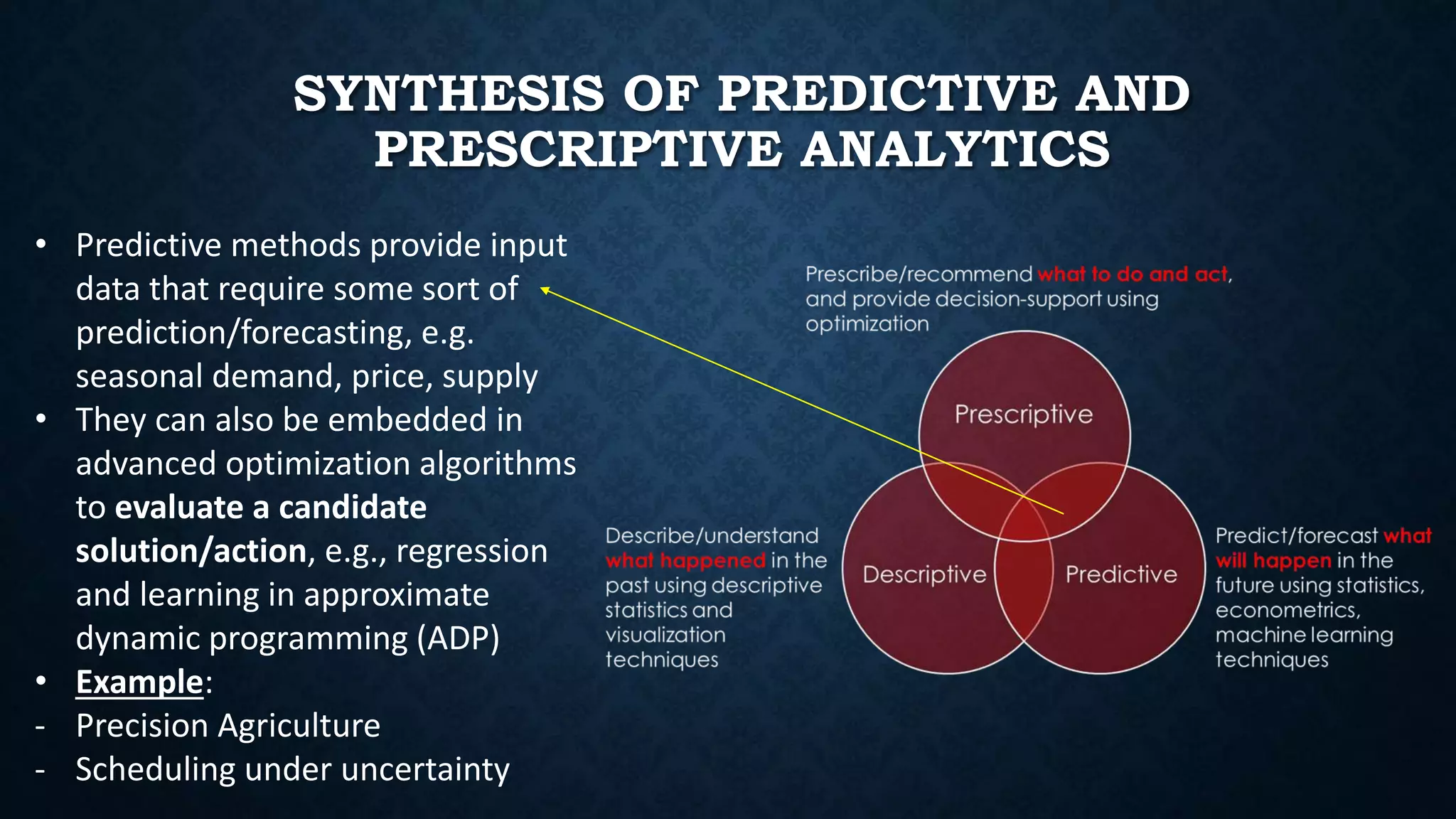
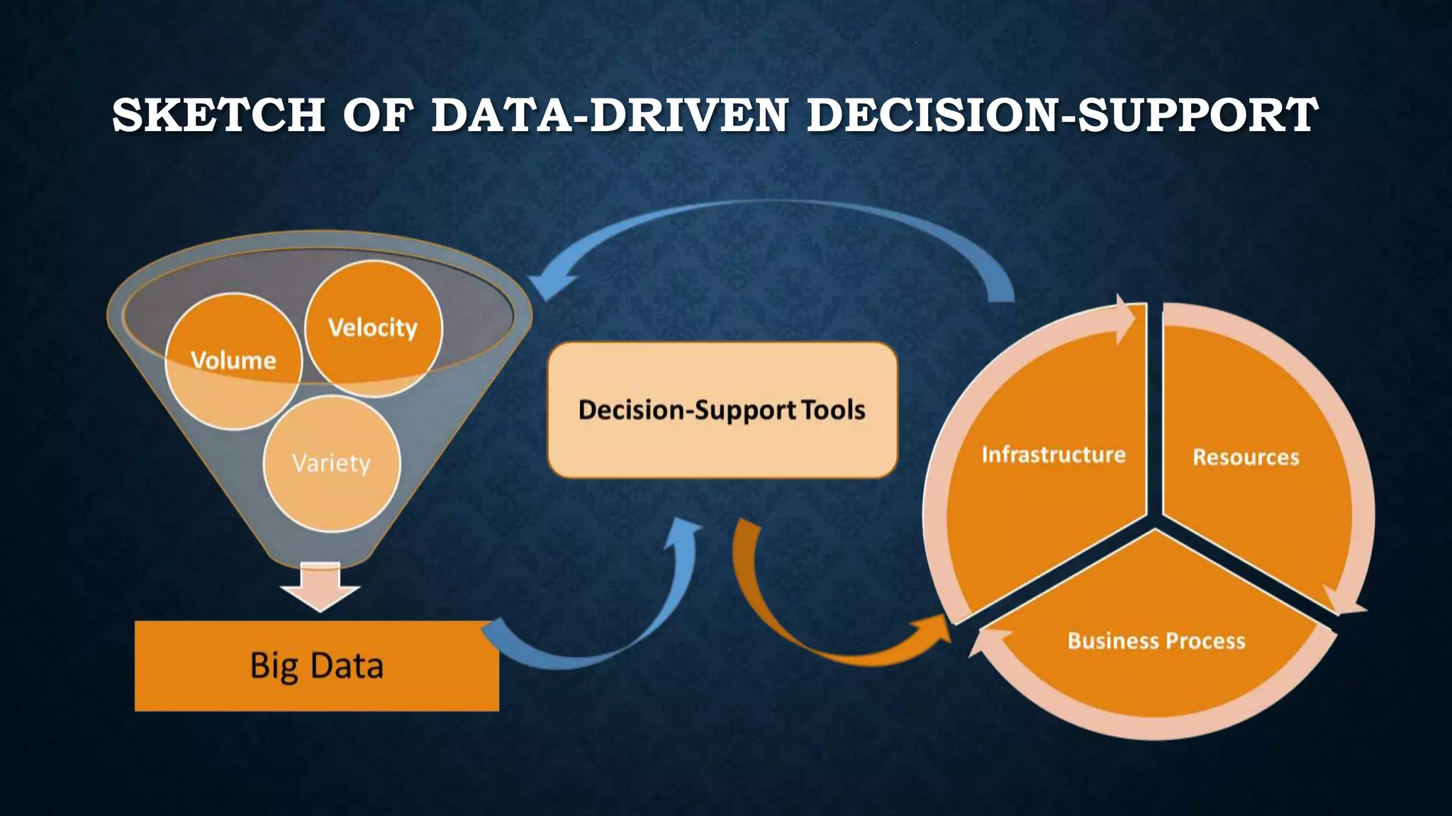
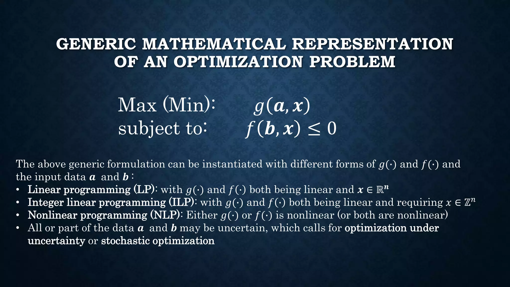
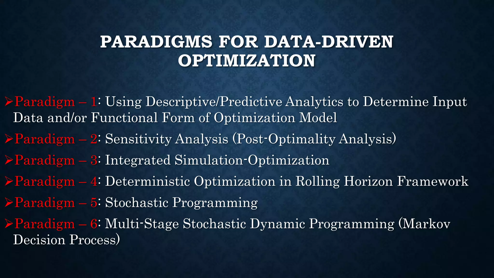
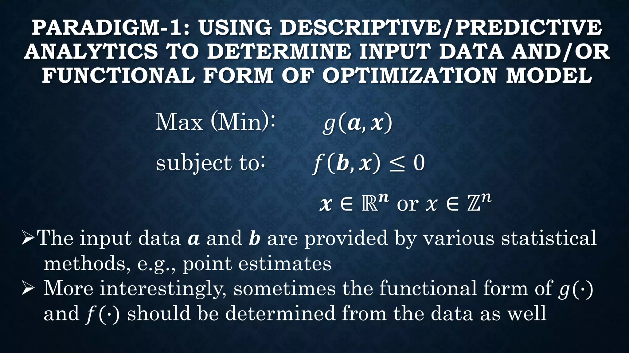
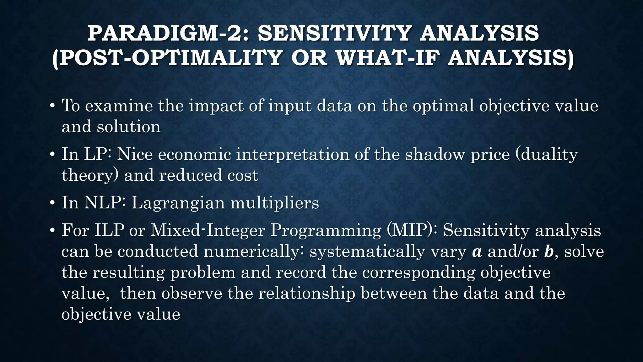
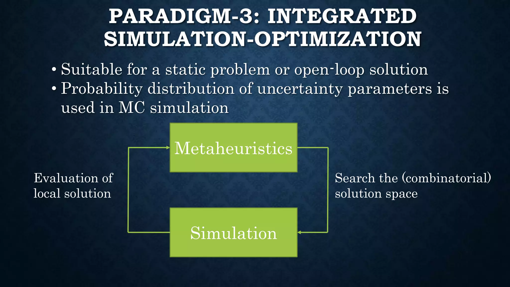
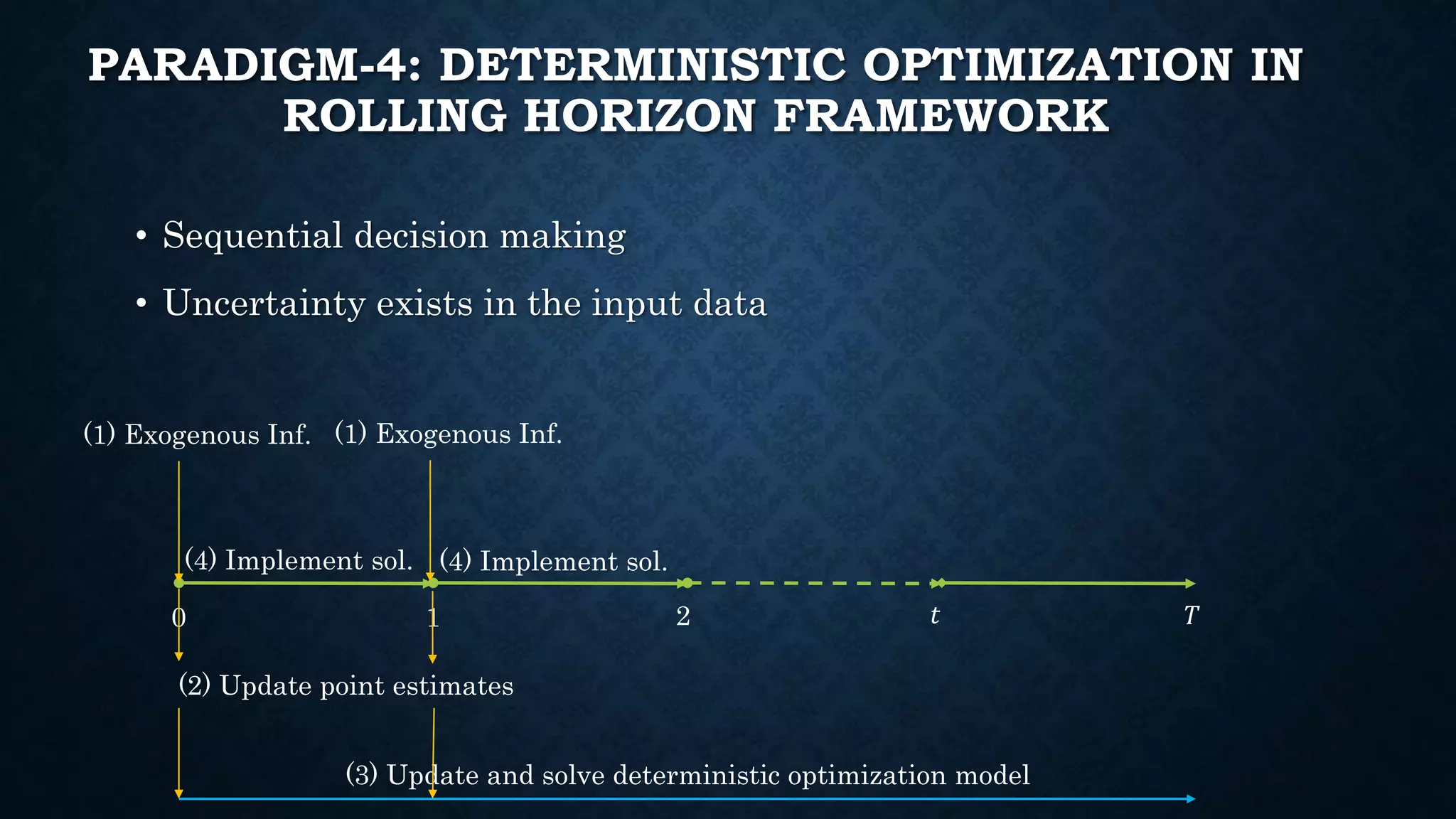
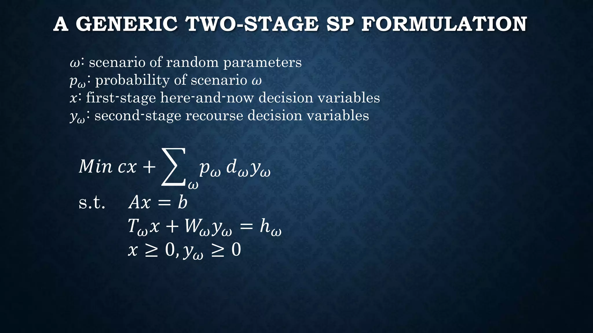
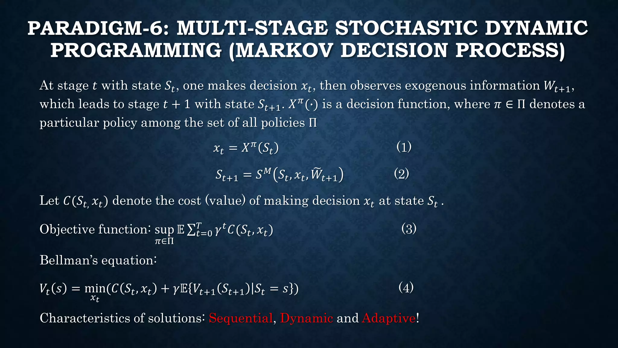
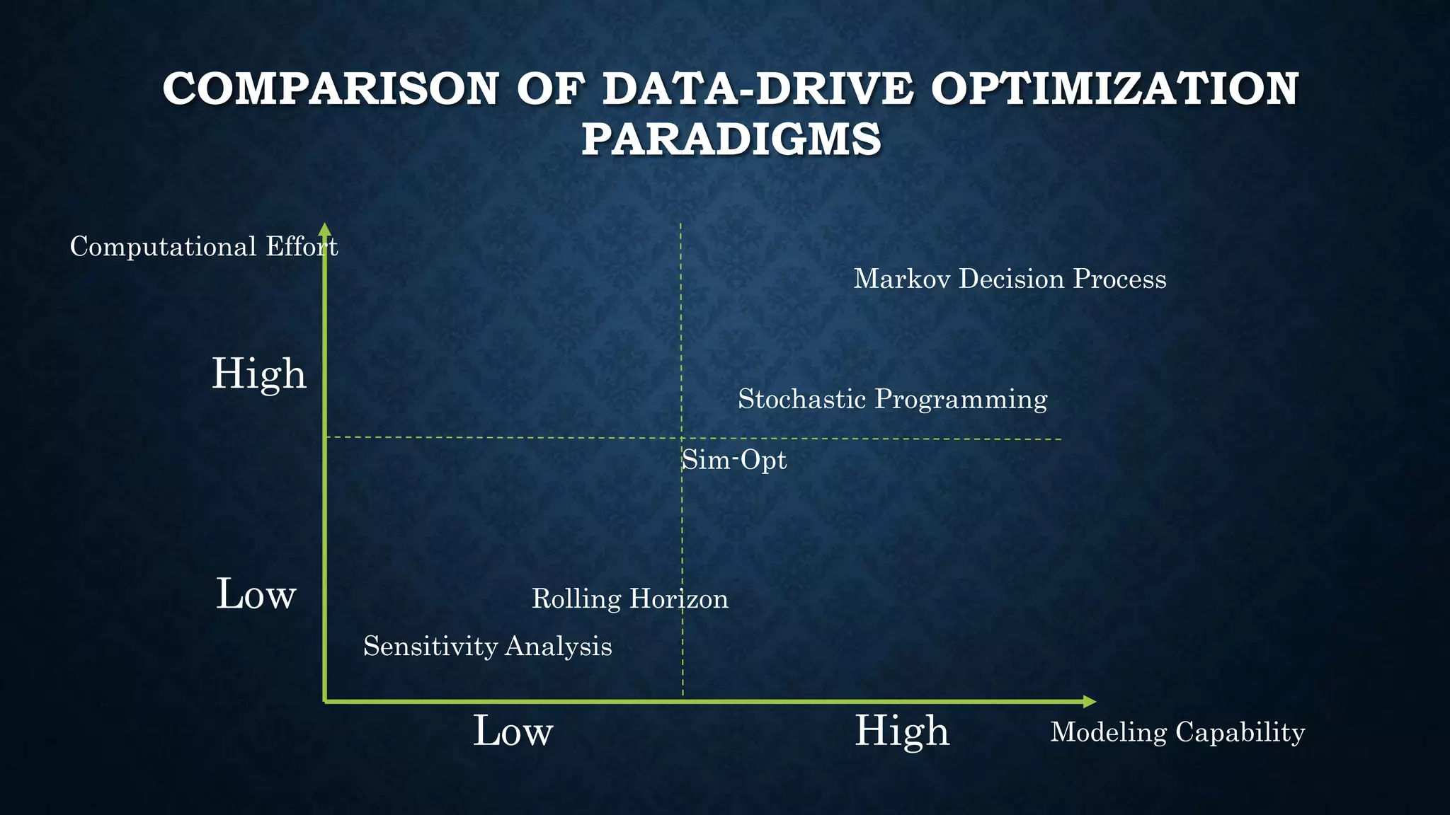
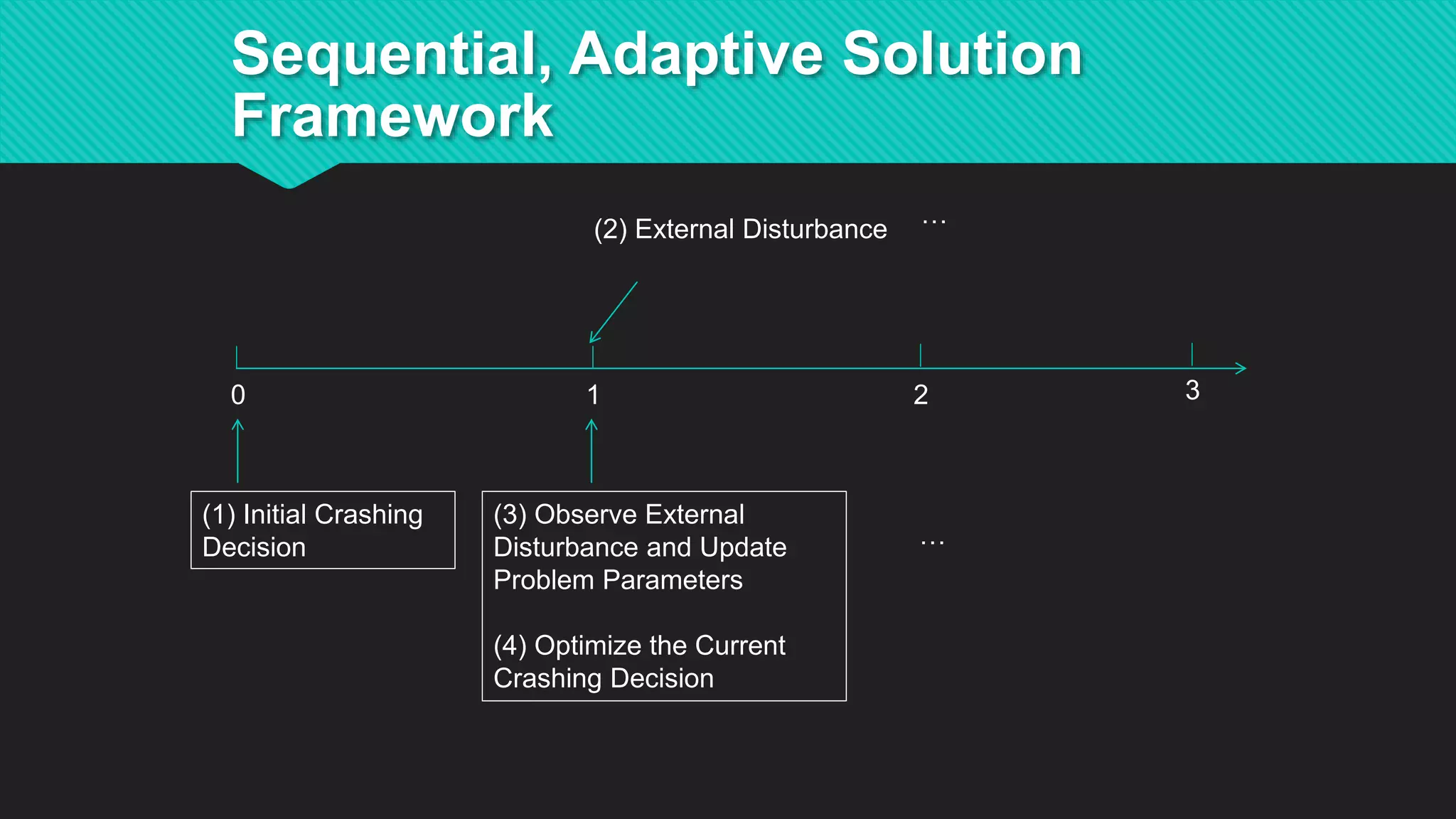
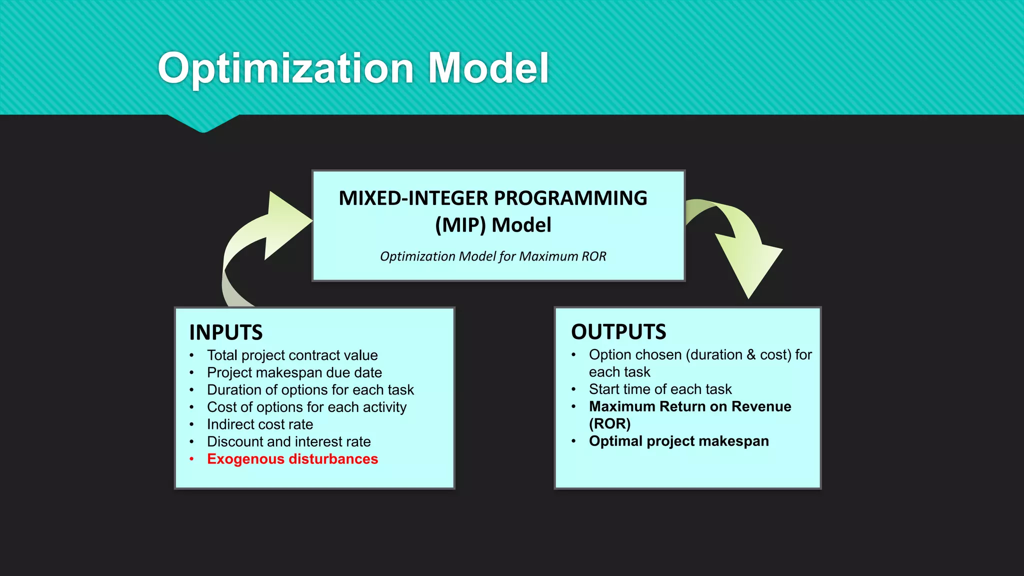
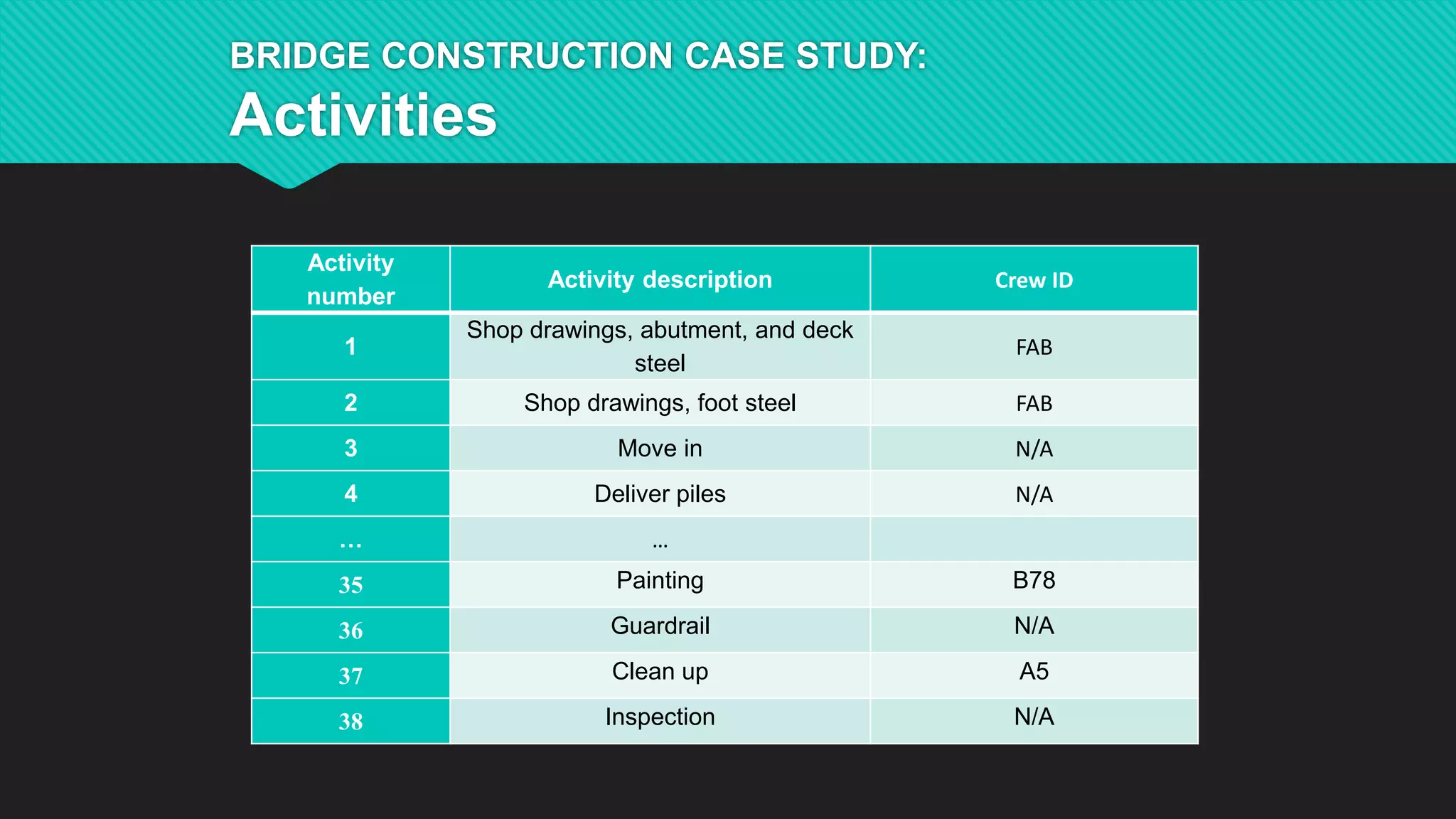
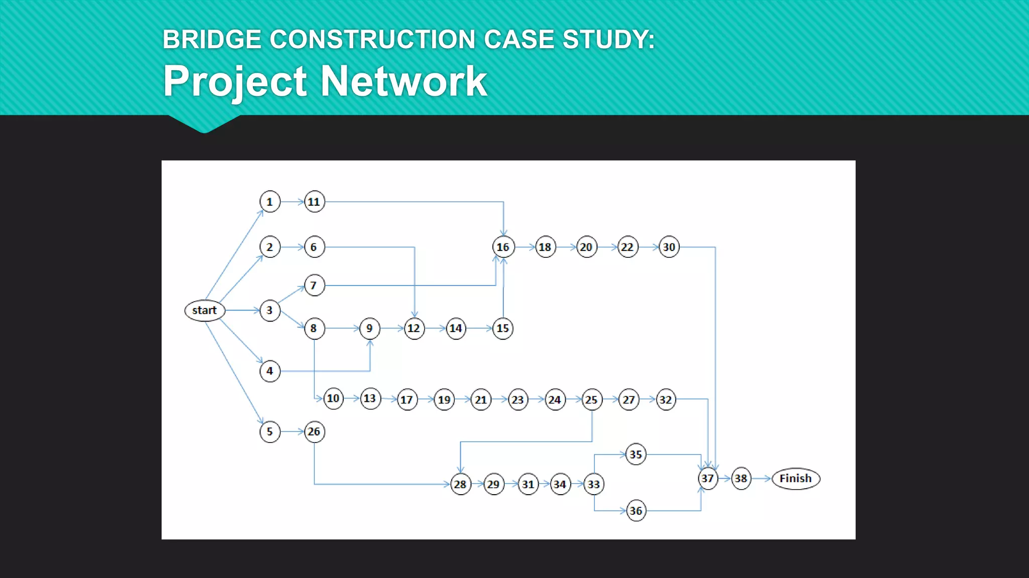
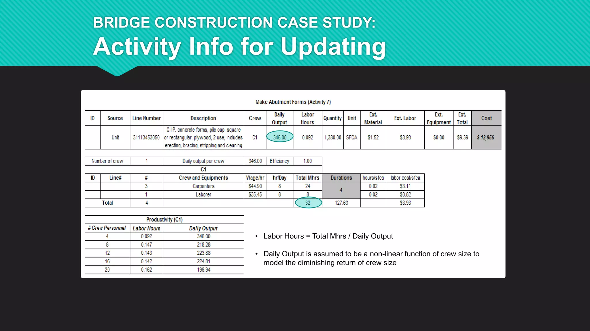
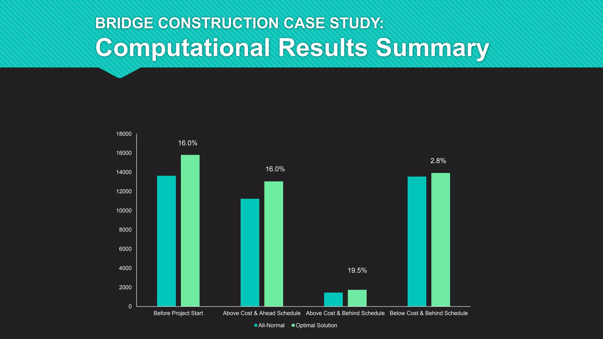
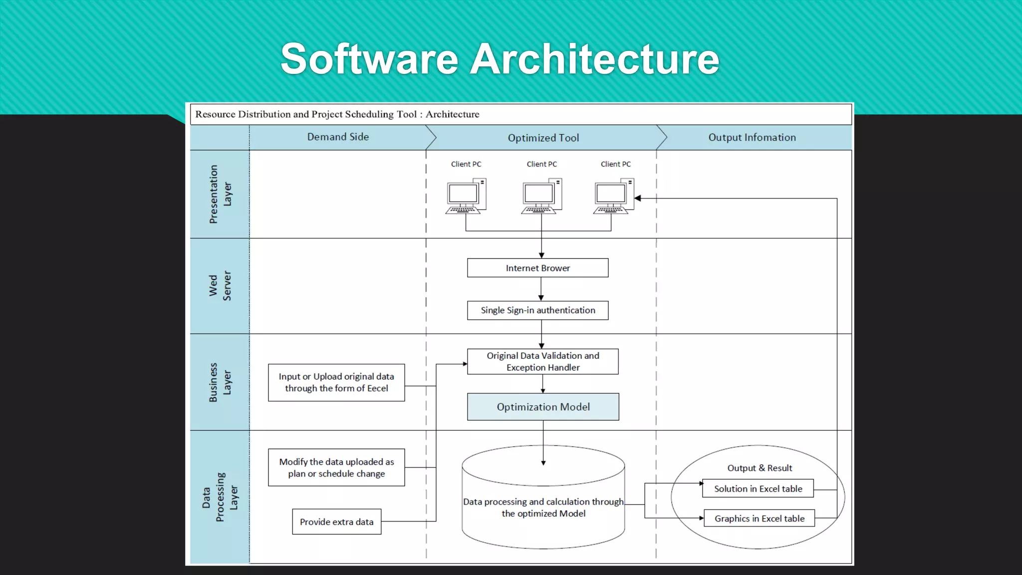
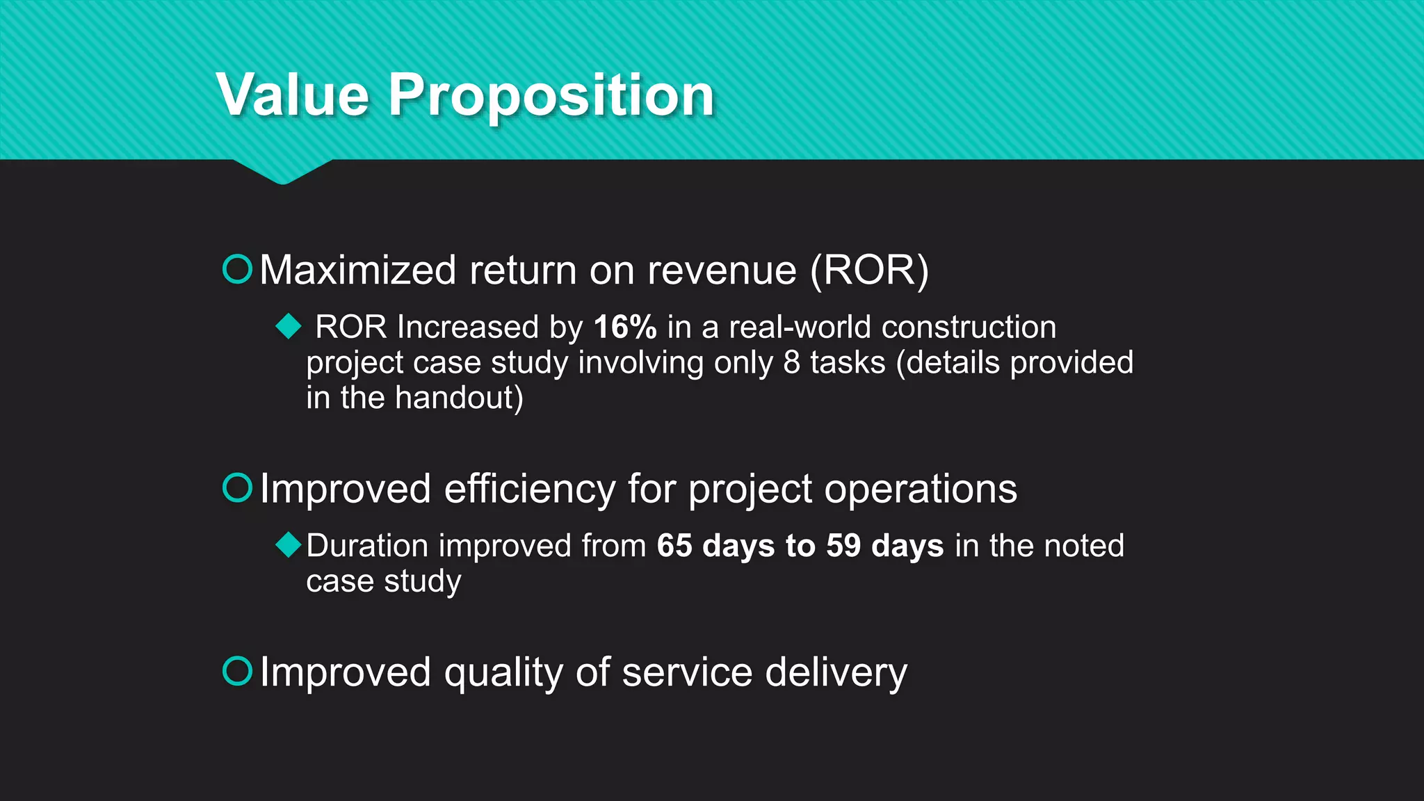
This document summarizes Dr. Haitao Li's presentation on synthesizing analytical methods for data-driven decision making. It discusses the three pillars of analytics - descriptive, predictive, and prescriptive. Various data-driven decision support paradigms are presented, including using descriptive/predictive analytics to determine optimization model inputs, sensitivity analysis, integrated simulation-optimization, and stochastic programming. An application example of a project scheduling and resource allocation tool for complex construction projects is provided, with details on its optimization model and software architecture.

1. SYNTHESIS OF ANALYTICAL METHODS
FOR DATA-DRIVEN DECISION MAKING
Haitao Li, Ph.D.
Supply Chain and Analytics Department
College of Business Administration
University of Missouri – St. Louis

2. UMSL SUPPLY CHAIN & ANALYTICS PROGRAMS
• BSBA with Supply Chain Emphasis
• MBA with two emphasis: Supply Chain Management and Business
Analytics
• PhD in Logistics and Supply Chain
• New MS in Supply Chain Analytics
• Well connected with the businesses in the greater St. Louis region
• “Citizen Data Scientists”

3. MY RESEARCH INTERESTS: APPLICATION
PERSPECTIVE
SCHEDULING
* RCPSP
* Machine
Scheduling
SUPPLY
CHAIN
OPTIMIZATIO
N
* SCCP
* Vehicle Routing
RESOURCE
ALLOCATION
* Sequential
Assignment
* Production
Planning

4. AGENDA
Three-Pillar of Analytics: Descriptive, Predictive and
Prescriptive
Data-Driven Decision-Support Paradigms
Application Example: Project Scheduling and Resource
Allocation Tool for Complex Construction Projects

5. THREE “PILLARS” OF ANALYTICS
Descriptive
Describe/understand
what happened in the
past using descriptive
statistics and
visualization
techniques
Predictive
Predict/forecast what
will happen in the
future using statistics,
econometrics, machine
learning, simulation
techniques
Prescriptive
Prescribe/recommend what to do and act, and
provide decision-support using optimization

6. DESCRIPTIVE ANALYTICS
Descriptive Statistics
Curve Fitting
Data Visualization
Statistical Inference

7. PREDICTIVE ANALYTICS
Multiple Regression Forecasting & Time
Series Analysis
Clustering Analysis
& Data Mining

8. PRESCRIPTIVE ANALYTICS: OPTIMIZATION
Information &
Data
Optimization Model,
Algorithm & Tool
Objective(s)
Technical
Requirements &
Business Rules
Best (better) Course
of Actions

9. A CONCISE MAP OF OPTIMIZATION
METHODOLOGIES
Optimization Models and
Methods
Deterministic
Optimization
Optimization under
Uncertainty
Mathematical
Programming Heuristics
Robust
Optimization
Stochastic
Optimization
LP, ILP, MIP,
NLP, MINLP
Network
Optimization
Stochastic
Programming
Markov Decision
Process (MDP)
Special-
Purpose
Metaheuristics
Constraint
Programming Sim-Opt

10. SYNTHESIS OF DESCRIPTIVE AND
PRESCRIPTIVE ANALYTICS
• Descriptive analytics provides
input data to a prescriptive
(optimization) model, e.g.,
point estimates, probability
distribution
• Example:
- Supply chain network design
- Planting and Harvest
planning

11. SYNTHESIS OF PREDICTIVE AND
PRESCRIPTIVE ANALYTICS
• Predictive methods provide input
data that require some sort of
prediction/forecasting, e.g.
seasonal demand, price, supply
• They can also be embedded in
advanced optimization algorithms
to evaluate a candidate
solution/action, e.g., regression
and learning in approximate
dynamic programming (ADP)
• Example:
- Precision Agriculture
- Scheduling under uncertainty

12. SKETCH OF DATA-DRIVEN DECISION-SUPPORT

13. GENERIC MATHEMATICAL REPRESENTATION
OF AN OPTIMIZATION PROBLEM
Max (Min): 𝑔 𝒂, 𝒙
subject to: 𝑓 𝒃, 𝒙 ≤ 0
The above generic formulation can be instantiated with different forms of 𝑔(∙) and 𝑓(∙) and
the input data 𝒂 and 𝒃 :
• Linear programming (LP): with 𝑔(∙) and 𝑓 ∙ both being linear and 𝒙 ∈ ℝ 𝒏
• Integer linear programming (ILP): with 𝑔(∙) and 𝑓 ∙ both being linear and requiring 𝑥 ∈ ℤ 𝑛
• Nonlinear programming (NLP): Either 𝑔(∙) or 𝑓(∙) is nonlinear (or both are nonlinear)
• All or part of the data 𝒂 and 𝒃 may be uncertain, which calls for optimization under
uncertainty or stochastic optimization

14. PARADIGMS FOR DATA-DRIVEN
OPTIMIZATION
Paradigm – 1: Using Descriptive/Predictive Analytics to Determine Input
Data and/or Functional Form of Optimization Model
Paradigm – 2: Sensitivity Analysis (Post-Optimality Analysis)
Paradigm – 3: Integrated Simulation-Optimization
Paradigm – 4: Deterministic Optimization in Rolling Horizon Framework
Paradigm – 5: Stochastic Programming
Paradigm – 6: Multi-Stage Stochastic Dynamic Programming (Markov
Decision Process)

15. PARADIGM-1: USING DESCRIPTIVE/PREDICTIVE
ANALYTICS TO DETERMINE INPUT DATA AND/OR
FUNCTIONAL FORM OF OPTIMIZATION MODEL
Max (Min): 𝑔 𝒂, 𝒙
subject to: 𝑓 𝒃, 𝒙 ≤ 0
𝒙 ∈ ℝ 𝒏
or 𝑥 ∈ ℤ 𝑛
The input data 𝒂 and 𝒃 are provided by various statistical
methods, e.g., point estimates
 More interestingly, sometimes the functional form of 𝑔(∙)
and 𝑓(∙) should be determined from the data as well

16. PARADIGM-2: SENSITIVITY ANALYSIS
(POST-OPTIMALITY OR WHAT-IF ANALYSIS)
• To examine the impact of input data on the optimal objective value
and solution
• In LP: Nice economic interpretation of the shadow price (duality
theory) and reduced cost
• In NLP: Lagrangian multipliers
• For ILP or Mixed-Integer Programming (MIP): Sensitivity analysis
can be conducted numerically: systematically vary 𝒂 and/or 𝒃, solve
the resulting problem and record the corresponding objective
value, then observe the relationship between the data and the
objective value

17. PARADIGM-3: INTEGRATED
SIMULATION-OPTIMIZATION
• Suitable for a static problem or open-loop solution
• Probability distribution of uncertainty parameters is
used in MC simulation
Metaheuristics
Simulation
Search the (combinatorial)
solution space
Evaluation of
local solution

18. PARADIGM-4: DETERMINISTIC OPTIMIZATION IN
ROLLING HORIZON FRAMEWORK
• Sequential decision making
• Uncertainty exists in the input data
0 1 2 𝑡 𝑇
(1) Exogenous Inf.
(2) Update point estimates
(3) Update and solve deterministic optimization model
(4) Implement sol.
(1) Exogenous Inf.
(4) Implement sol.

19. PARADIGM-5: TWO-STAGE STOCHASTIC
PROGRAMMING (SP)
First-stage: here-and-now decisions to match resources with
jobs
Second-stage: recourse decisions to identify whether a job is
lost or a resource is idle
The objective is to minimize the total expected overall cost
First-stage assignment cost
Expected second-stage cost (relying on the probability
distribution of random parameters)

20. A GENERIC TWO-STAGE SP FORMULATION
𝜔: scenario of random parameters
𝑝 𝜔: probability of scenario 𝜔
𝑥: first-stage here-and-now decision variables
𝑦 𝜔: second-stage recourse decision variables
𝑀𝑖𝑛 𝑐𝑥 +
𝜔
𝑝 𝜔 𝑑 𝜔 𝑦 𝜔
s.t. 𝐴𝑥 = 𝑏
𝑇 𝜔 𝑥 + 𝑊𝜔 𝑦 𝜔 = ℎ 𝜔
𝑥 ≥ 0, 𝑦 𝜔 ≥ 0

21. PARADIGM-6: MULTI-STAGE STOCHASTIC DYNAMIC
PROGRAMMING (MARKOV DECISION PROCESS)
At stage 𝑡 with state 𝑆𝑡, one makes decision 𝑥𝑡, then observes exogenous information 𝑊𝑡+1,
which leads to stage 𝑡 + 1 with state 𝑆𝑡+1. 𝑋 𝜋(∙) is a decision function, where 𝜋 ∈ Π denotes a
particular policy among the set of all policies Π
𝑥𝑡 = 𝑋 𝜋 𝑆𝑡 (1)
𝑆𝑡+1 = 𝑆 𝑀
𝑆𝑡, 𝑥 𝑡, 𝑊𝑡+1 (2)
Let 𝐶(𝑆𝑡, 𝑥𝑡) denote the cost (value) of making decision 𝑥𝑡 at state 𝑆𝑡 .
Objective function: sup
𝜋∈Π
𝔼 𝑡=0
𝑇
𝛾 𝑡 𝐶(𝑆𝑡, 𝑥𝑡) (3)
Bellman’s equation:
𝑉𝑡 𝑠 = min
𝑥 𝑡
(𝐶 𝑆𝑡, 𝑥𝑡 + 𝛾𝔼 𝑉𝑡+1 𝑆𝑡+1 𝑆𝑡 = 𝑠 ) (4)
Characteristics of solutions: Sequential, Dynamic and Adaptive!

22. COMPARISON OF DATA-DRIVE OPTIMIZATION
PARADIGMS
Modeling Capability
Computational Effort
Sensitivity Analysis
Rolling Horizon
Stochastic Programming
Low High
Low
High
Sim-Opt
Markov Decision Process

23. PROJECT SCHEDULING AND RESOURCE
ALLOCATION TOOL FOR COMPLEX
CONSTRUCTION PROJECTS
Provisional (62/454,511) filed 02/03/17
PCT/US2018/16369 filed 02/01/18
US National Stage application filed 08/03/19

24. Such industries include:
o Construction
o Pharmaceutical
o Oil & Gas
o Military
o Supply Chain
o Logistics
Across many industries, optimizing resource management,
supply chain design and logistics is essential in minimizing
costs and keeping projects on time.
Project Management Optimization Needs
What is the Problem?

25.  Cost over-runs are not uncommon because resources are not
optimally allocated to project tasks
 Uncertainty in task duration caused by variations in crew productivity
 Difficulty of scheduling payments to meet complex payment terms
Current tools designed to save time and money by optimizing project
management are lacking – they aren’t dynamic and very few provide
real-time feedback or other useful functionality.
What is the Problem?
Project Management Challenges

26.  Optimizes the time-cost tradeoff (crashing) decisions with
complex payment structure and discounted cash flows
 Sequential and adaptive solution approach to capture the
variation of project operations efficiency and productivity
 A data-driven approach closing the gap between decision
support and the “big data” made available through IT
advancement
How Does This Technology Solve
the Problem?

27. (2) External Disturbance
0 1 2 3
(1) Initial Crashing
Decision
(3) Observe External
Disturbance and Update
Problem Parameters
(4) Optimize the Current
Crashing Decision
…
…
Sequential, Adaptive Solution
Framework

28. Optimization Model
OUTPUTS
• Option chosen (duration & cost) for
each task
• Start time of each task
• Maximum Return on Revenue
(ROR)
• Optimal project makespan
MIXED-INTEGER PROGRAMMING
(MIP) Model
Optimization Model for Maximum ROR
INPUTS
• Total project contract value
• Project makespan due date
• Duration of options for each task
• Cost of options for each activity
• Indirect cost rate
• Discount and interest rate
• Exogenous disturbances

29. Activity
number
Activity description Crew ID
1
Shop drawings, abutment, and deck
steel
FAB
2 Shop drawings, foot steel FAB
3 Move in N/A
4 Deliver piles N/A
… …
35 Painting B78
36 Guardrail N/A
37 Clean up A5
38 Inspection N/A
BRIDGE CONSTRUCTION CASE STUDY:
Activities

30. BRIDGE CONSTRUCTION CASE STUDY:
Project Network

31. • Labor Hours = Total Mhrs / Daily Output
• Daily Output is assumed to be a non-linear function of crew size to
model the diminishing return of crew size
BRIDGE CONSTRUCTION CASE STUDY:
Activity Info for Updating

32. 0
2000
4000
6000
8000
10000
12000
14000
16000
18000
Before Project Start Above Cost & Ahead Schedule Above Cost & Behind Schedule Below Cost & Behind Schedule
All-Normal Optimal Solution
16.0%
16.0%
19.5%
2.8%
BRIDGE CONSTRUCTION CASE STUDY:
Computational Results Summary

33. Software Architecture

34.  A prototype has been developed with:
web-based architecture using ASP technology (eliminates the
need for user to purchase optimization solver);
successful integration of GUI, database and optimization
models; and
controlled user portal and privilege
Development Stage

35. Maximized return on revenue (ROR)
 ROR Increased by 16% in a real-world construction
project case study involving only 8 tasks (details provided
in the handout)
Improved efficiency for project operations
Duration improved from 65 days to 59 days in the noted
case study
Improved quality of service delivery
Value Proposition

36. QUESTIONS?
COMMENTS?
THANK YOU!