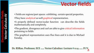
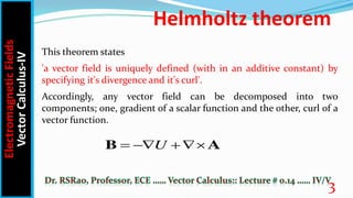
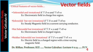
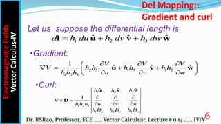
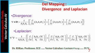
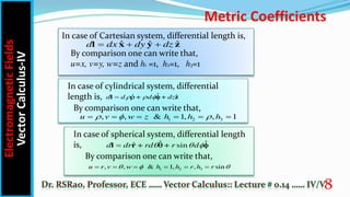
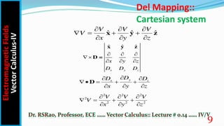
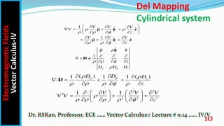
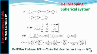
Series: EMF Theory
Lecture: # 0.14
Dr R S Rao
Professor, ECE
Vector fields, graphical representations for divergence and curl, gradient,
divergence and curl mapping into different coordinate systems
Passionate
Teaching
Joyful
Learning
Electromagnetic
Fields
Vector
Calculus-IV Vector fields
2
• Fields are regions/part spaces exhibiting certain special properties.
•They have analytical as well graphical representation.
•A properly defined vector/scalar function can describe the fields
mathematically and completely.
•The gradient, divergence and curl are able to give critical information
pertaining to fields.
•The graphical representation uses flux lines and it is due to Michael
Faraday.
Helmholtz theorem
This theorem states
'a vector field is uniquely defined (with in an additive constant) by
specifying it's divergence and it's curl'.
Accordingly, any vector field can be decomposed into two
components; one, gradient of a scalar function and the other, curl of a
vector function.
U
  
B A
Electromagnetic
Fields
Vector
Calculus-IV
3
Electromagnetic
Fields
Vector
Calculus-IV
• Solenoidal and irrotational if .F=0 and ×F=0
Ex: Electrostatic field in charge free region.
•Solenoidal but not irrotational if .F=0 and ×F≠0
Ex: Steady Magnetic field in a current carrying conductor.
•Not Solenoidal but irrotational if .F ≠ 0 and ×F=0
Ex: Electrostatic field in charged region.
•Neither Solenoidal nor irrotational if .F ≠ 0 and ×F ≠ 0
Ex: Electric field in a charged region with a time varying
magnetic field.
Vector fields
4
Critical Features of vector fields….
Vector fields
•The field in (a) is found to have nonzero curl and
zero divergence. The field lines can be seen
rotating without any divergence.
•The field in (b) is found to have zero curl with
nonzero divergence. The field lines can be seen
diverging without any rotation.
•The field in (c) is found to have nonzero curl and
nonzero divergence. The field lines can be seen
rotating with divergence.
•The field in (d) is found to have zero curl with
zero divergence. The field lines can be seen
neither diverging nor rotating.
Electromagnetic
Fields
Vector
Calculus-IV
5
•Conclusion is, the div and curl, found from analytical expressions, correlate with
diverging and rotational features of field lines. However, there are exceptions.
Features of graphical representation….
2 3 1 3 1 2
1 2 3
1
ˆ ˆ ˆ
u v w
V V V
V h h h h h h
h h h u v w
  
 
   
 
  
 
1 2 3
1 2 3
1 2 3
ˆ ˆ ˆ
1
u v w
D
u v w
h h h
h h h u v w
h D h D h D
  
  
  
•Curl:
•Gradient:
1 2 3
ˆ ˆ ˆ
l u v w
d h du h dv h dw
  
Let us suppose the differential length is
Del Mapping::
Gradient and curl
Electromagnetic
Fields
Vector
Calculus-IV
6
     
2 3 3 1 1 2
1 2 3
1
D u v w
h h D h h D h h D
h h h u v w
 
  
     
    
 
     
  
     
 
2 2 3 3 1 1 2
1 2 3 1 2 3
1 h h h h h h
V V V
V
h h h u h u v h v w h w
 
     
   
     
 
 
   
 
     
     
     
 
     
 
   
 
•Laplacian:
•Divergence:
Del Mapping::
Divergence and Laplacian
Electromagnetic
Fields
Vector
Calculus-IV
7
In case of Cartesian system, differential length is,
ˆ ˆ ˆ
l x y z
d dx dy dz
  
By comparison one can write that,
u=x, v=y, w=z and h1 =1, h2=1, h3=1
In case of cylindrical system, differential
length is,
By comparison one can write that,
1 2 3
, , & 1, , 1
u v w z h h h
  
     
ˆ
ˆ ˆ
d d d dz
  

l z
   
In case of spherical system, differential length
is, ˆ ˆ
ˆ sin
d dr rd r d
  

l r    
By comparison one can write that,
1 2 3
, , & 1, , sin
u r v w h h r h r
  
     
Metric Coefficients
Electromagnetic
Fields
Vector
Calculus-IV
8
Del Mapping::
Cartesian system
y
x z
D
D D
x y z

 
    
  
D
2 2 2
2
2 2 2
V V V
V
x y z
  
   
  
ˆ ˆ ˆ
V V V
V
x y z
  
   
  
x y z
ˆ ˆ ˆ
x y z
x y z
D D D
  
 
  
x y z
D =
Electromagnetic
Fields
Vector
Calculus-IV
9
Del Mapping
Cylindrical system
1 ˆ
ˆ ˆ
V V
V   
  
 
  
   
 
  
 
ρ z
̂
1 ˆ
ˆ ˆ
V V

  
  
  
  
ρ z
̂
ˆ
ˆ ˆ
V
z
  
  
 
  
   
 
  
 
ρ z
ˆ
ˆ ˆ
V
z

  
  
  
  
ρ z
ˆ
ˆ ˆ
1
z
z
D D D
 

  

  
 
  
z
D =
 
( ) ( )
1 1 1 z
D D D
z
 
 
    
  
   
  
D
2 2
2
2 2 2
1 1
V V V
V
z

    
 
 
   
   
 
 
   
   
Electromagnetic
Fields
Vector
Calculus-IV
10
Del Mapping::
Spherical system
2
ˆ ˆ
ˆ sin
1
sin
sin
r
r r
r r
D rD r D
 

  

  
  
  
r
D
 
2
2
1
( sin ) ( sin ) ( )
sin
r
r D r D rD
r r
 
 
  
 
 
  
   
   
 
 
   
  
     
 
D
2
2 2
2 2 2 2 2
1 1 1
sin
sin sin
V V V
V r
r r r r r

    
 
    
   
     
   
    
     
Electromagnetic
Fields
Vector
Calculus-IV
11
2
2
1 ˆ ˆ
ˆ
sin sin
sin
V V V
V r r r
r r
  
  
 
  
   
 
  
 
r θ ̂
1 1
ˆ ˆ
ˆ
V V V

  
  
  
  
θ ̂
ˆ ˆ
ˆ
  
  
 
  
   
 
  
 
θ
ˆ ˆ
ˆ
sin
r r
  
  
 
  
   
 
  
 
θ ̂
1 1
ˆ ˆ
ˆ
sin
V V V
r r

  
  
  
  
r θ ̂
ˆ ˆ
ˆ
r r
  
  
 
  
   
 
  
 
θ
ENOUGH
FOR
TODAY
ENOUGH
FOR
TODAY
ENOUGH
FOR
TODAY
ENOUGH
FOR
TODAY
ENOUGH
FOR
TODAY
12

EMF.0.14.VectorCalculus-IV.pdf

  • 1.
    Series: EMF Theory Lecture:# 0.14 Dr R S Rao Professor, ECE Vector fields, graphical representations for divergence and curl, gradient, divergence and curl mapping into different coordinate systems Passionate Teaching Joyful Learning
  • 2.
    Electromagnetic Fields Vector Calculus-IV Vector fields 2 •Fields are regions/part spaces exhibiting certain special properties. •They have analytical as well graphical representation. •A properly defined vector/scalar function can describe the fields mathematically and completely. •The gradient, divergence and curl are able to give critical information pertaining to fields. •The graphical representation uses flux lines and it is due to Michael Faraday.
  • 3.
    Helmholtz theorem This theoremstates 'a vector field is uniquely defined (with in an additive constant) by specifying it's divergence and it's curl'. Accordingly, any vector field can be decomposed into two components; one, gradient of a scalar function and the other, curl of a vector function. U    B A Electromagnetic Fields Vector Calculus-IV 3
  • 4.
    Electromagnetic Fields Vector Calculus-IV • Solenoidal andirrotational if .F=0 and ×F=0 Ex: Electrostatic field in charge free region. •Solenoidal but not irrotational if .F=0 and ×F≠0 Ex: Steady Magnetic field in a current carrying conductor. •Not Solenoidal but irrotational if .F ≠ 0 and ×F=0 Ex: Electrostatic field in charged region. •Neither Solenoidal nor irrotational if .F ≠ 0 and ×F ≠ 0 Ex: Electric field in a charged region with a time varying magnetic field. Vector fields 4 Critical Features of vector fields….
  • 5.
    Vector fields •The fieldin (a) is found to have nonzero curl and zero divergence. The field lines can be seen rotating without any divergence. •The field in (b) is found to have zero curl with nonzero divergence. The field lines can be seen diverging without any rotation. •The field in (c) is found to have nonzero curl and nonzero divergence. The field lines can be seen rotating with divergence. •The field in (d) is found to have zero curl with zero divergence. The field lines can be seen neither diverging nor rotating. Electromagnetic Fields Vector Calculus-IV 5 •Conclusion is, the div and curl, found from analytical expressions, correlate with diverging and rotational features of field lines. However, there are exceptions. Features of graphical representation….
  • 6.
    2 3 13 1 2 1 2 3 1 ˆ ˆ ˆ u v w V V V V h h h h h h h h h u v w                 1 2 3 1 2 3 1 2 3 ˆ ˆ ˆ 1 u v w D u v w h h h h h h u v w h D h D h D          •Curl: •Gradient: 1 2 3 ˆ ˆ ˆ l u v w d h du h dv h dw    Let us suppose the differential length is Del Mapping:: Gradient and curl Electromagnetic Fields Vector Calculus-IV 6
  • 7.
         2 3 3 1 1 2 1 2 3 1 D u v w h h D h h D h h D h h h u v w                                    2 2 3 3 1 1 2 1 2 3 1 2 3 1 h h h h h h V V V V h h h u h u v h v w h w                                                               •Laplacian: •Divergence: Del Mapping:: Divergence and Laplacian Electromagnetic Fields Vector Calculus-IV 7
  • 8.
    In case ofCartesian system, differential length is, ˆ ˆ ˆ l x y z d dx dy dz    By comparison one can write that, u=x, v=y, w=z and h1 =1, h2=1, h3=1 In case of cylindrical system, differential length is, By comparison one can write that, 1 2 3 , , & 1, , 1 u v w z h h h          ˆ ˆ ˆ d d d dz     l z     In case of spherical system, differential length is, ˆ ˆ ˆ sin d dr rd r d     l r     By comparison one can write that, 1 2 3 , , & 1, , sin u r v w h h r h r          Metric Coefficients Electromagnetic Fields Vector Calculus-IV 8
  • 9.
    Del Mapping:: Cartesian system y xz D D D x y z            D 2 2 2 2 2 2 2 V V V V x y z           ˆ ˆ ˆ V V V V x y z           x y z ˆ ˆ ˆ x y z x y z D D D         x y z D = Electromagnetic Fields Vector Calculus-IV 9
  • 10.
    Del Mapping Cylindrical system 1ˆ ˆ ˆ V V V                       ρ z ̂ 1 ˆ ˆ ˆ V V              ρ z ̂ ˆ ˆ ˆ V z                       ρ z ˆ ˆ ˆ V z              ρ z ˆ ˆ ˆ 1 z z D D D                z D =   ( ) ( ) 1 1 1 z D D D z                    D 2 2 2 2 2 2 1 1 V V V V z                               Electromagnetic Fields Vector Calculus-IV 10
  • 11.
    Del Mapping:: Spherical system 2 ˆˆ ˆ sin 1 sin sin r r r r r D rD r D                 r D   2 2 1 ( sin ) ( sin ) ( ) sin r r D r D rD r r                                          D 2 2 2 2 2 2 2 2 1 1 1 sin sin sin V V V V r r r r r r                                       Electromagnetic Fields Vector Calculus-IV 11 2 2 1 ˆ ˆ ˆ sin sin sin V V V V r r r r r                       r θ ̂ 1 1 ˆ ˆ ˆ V V V              θ ̂ ˆ ˆ ˆ                       θ ˆ ˆ ˆ sin r r                       θ ̂ 1 1 ˆ ˆ ˆ sin V V V r r              r θ ̂ ˆ ˆ ˆ r r                       θ
  • 12.