Downloaded 41 times


![www.letsnurture.com
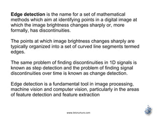
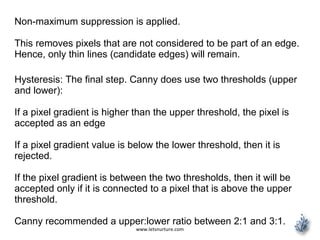
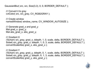
/** @function main */
int main( int argc, char** argv )
{
/// Load an image
src = imread( argv[1] );
if( !src.data )
{ return -1; }
/// Create a matrix of the same type and size as src (for dst)
dst.create( src.size(), src.type() );
/// Convert the image to grayscale
cvtColor( src, src_gray, CV_BGR2GRAY );
/// Create a window
namedWindow( window_name, CV_WINDOW_AUTOSIZE );
/// Create a Trackbar for user to enter threshold
createTrackbar( "Min Threshold:", window_name, &lowThreshold,
max_lowThreshold, CannyThreshold );
/// Show the image
CannyThreshold(0, 0);
/// Wait until user exit program by pressing a key
waitKey(0);
return 0;
}](https://image.slidesharecdn.com/edgedetectioniosapps-150519110911-lva1-app6891/85/Edge-detection-iOS-application-14-320.jpg)

![www.letsnurture.com
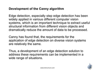
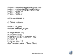
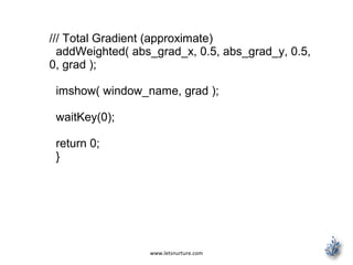
Loads the source image:
/// Load an image
src = imread( argv[1] );
if( !src.data )
{ return -1; }
Create a matrix of the same type and size of src (to be dst)
dst.create( src.size(), src.type() );
Convert the image to grayscale (using the function
cvtColor:
cvtColor( src, src_gray, CV_BGR2GRAY );](https://image.slidesharecdn.com/edgedetectioniosapps-150519110911-lva1-app6891/85/Edge-detection-iOS-application-16-320.jpg)

![www.letsnurture.com
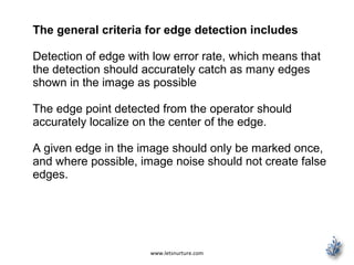
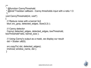
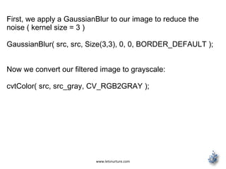
#include "opencv2/imgproc/imgproc.hpp"
#include "opencv2/highgui/highgui.hpp"
#include <stdlib.h>
#include <stdio.h>
using namespace cv;
/** @function main */
int main( int argc, char** argv )
{
Mat src, src_gray;
Mat grad;
char* window_name = "Sobel Demo - Simple Edge Detector";
int scale = 1;
int delta = 0;
int ddepth = CV_16S;
int c;
/// Load an image
src = imread( argv[1] );
if( !src.data )
{ return -1; }](https://image.slidesharecdn.com/edgedetectioniosapps-150519110911-lva1-app6891/85/Edge-detection-iOS-application-27-320.jpg)
![www.letsnurture.com
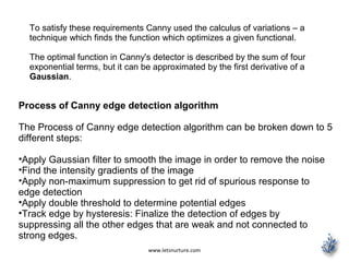
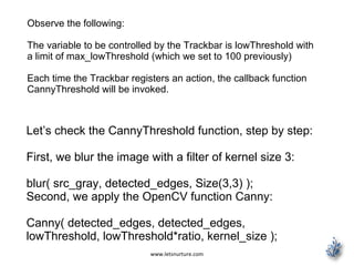
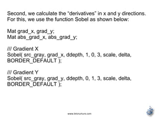
First we declare the variables we are going to use:
Mat src, src_gray;
Mat grad;
char* window_name = "Sobel Demo - Simple Edge
Detector";
int scale = 1;
int delta = 0;
int ddepth = CV_16S;
As usual we load our source image src:
src = imread( argv[1] );
if( !src.data )
{ return -1; }](https://image.slidesharecdn.com/edgedetectioniosapps-150519110911-lva1-app6891/85/Edge-detection-iOS-application-30-320.jpg)


![www.letsnurture.com
#include "opencv2/highgui/highgui.hpp"
#include "opencv2/imgproc/imgproc.hpp"
#include <iostream>
using namespace cv;
using namespace std;
void help()
{
cout << "nThis program demonstrates line finding with the Hough
transform.n"
"Usage:n"
"./houghlines <image_name>, Default is pic1.jpgn" << endl;
}
int main(int argc, char** argv)
{
const char* filename = argc >= 2 ? argv[1] : "pic1.jpg";
Mat src = imread(filename, 0);
if(src.empty())
{
help();
cout << "can not open " << filename << endl;
return -1;
}](https://image.slidesharecdn.com/edgedetectioniosapps-150519110911-lva1-app6891/85/Edge-detection-iOS-application-42-320.jpg)
![www.letsnurture.com
Mat dst, cdst;
Canny(src, dst, 50, 200, 3);
cvtColor(dst, cdst, CV_GRAY2BGR);
#if 0
vector<Vec2f> lines;
HoughLines(dst, lines, 1, CV_PI/180, 100, 0, 0 );
for( size_t i = 0; i < lines.size(); i++ )
{
float rho = lines[i][0], theta = lines[i][1];
Point pt1, pt2;
double a = cos(theta), b = sin(theta);
double x0 = a*rho, y0 = b*rho;
pt1.x = cvRound(x0 + 1000*(-b));
pt1.y = cvRound(y0 + 1000*(a));
pt2.x = cvRound(x0 - 1000*(-b));
pt2.y = cvRound(y0 - 1000*(a));
line( cdst, pt1, pt2, Scalar(0,0,255), 3, CV_AA);
}](https://image.slidesharecdn.com/edgedetectioniosapps-150519110911-lva1-app6891/85/Edge-detection-iOS-application-43-320.jpg)
![www.letsnurture.com
#else
vector<Vec4i> lines;
HoughLinesP(dst, lines, 1, CV_PI/180, 50, 50, 10 );
for( size_t i = 0; i < lines.size(); i++ )
{
Vec4i l = lines[i];
line( cdst, Point(l[0], l[1]), Point(l[2], l[3]),
Scalar(0,0,255), 3, CV_AA);
}
#endif
imshow("source", src);
imshow("detected lines", cdst);
waitKey();
return 0;
}](https://image.slidesharecdn.com/edgedetectioniosapps-150519110911-lva1-app6891/85/Edge-detection-iOS-application-44-320.jpg)
![www.letsnurture.com
And then you display the result by drawing the lines.
for( size_t i = 0; i < lines.size(); i++ )
{
float rho = lines[i][0], theta = lines[i][1];
Point pt1, pt2;
double a = cos(theta), b = sin(theta);
double x0 = a*rho, y0 = b*rho;
pt1.x = cvRound(x0 + 1000*(-b));
pt1.y = cvRound(y0 + 1000*(a));
pt2.x = cvRound(x0 - 1000*(-b));
pt2.y = cvRound(y0 - 1000*(a));
line( cdst, pt1, pt2, Scalar(0,0,255), 3, CV_AA);
}](https://image.slidesharecdn.com/edgedetectioniosapps-150519110911-lva1-app6891/85/Edge-detection-iOS-application-47-320.jpg)

![www.letsnurture.com
minLinLength: The minimum number of points that
can form a line. Lines with less than this number of
points are disregarded.
maxLineGap: The maximum gap between two points
to be considered in the same line.
And then you display the result by drawing the lines.
for( size_t i = 0; i < lines.size(); i++ )
{
Vec4i l = lines[i];
line( cdst, Point(l[0], l[1]), Point(l[2], l[3]),
Scalar(0,0,255), 3, CV_AA);
}](https://image.slidesharecdn.com/edgedetectioniosapps-150519110911-lva1-app6891/85/Edge-detection-iOS-application-49-320.jpg)


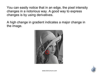
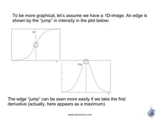
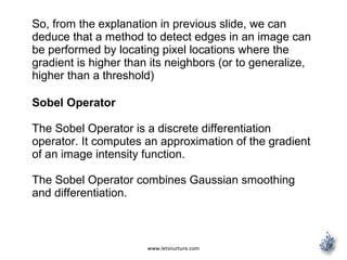
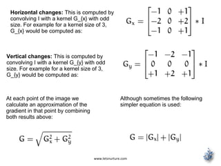
The document provides an overview of edge detection, specifically focusing on the Canny edge detection algorithm, which identifies sharp changes in image brightness to detect edges. It details the five main steps of the Canny algorithm including noise reduction, gradient calculation, non-maximum suppression, double thresholding, and edge tracking. Additionally, the document includes code snippets for implementing the Canny detector and discusses alternative methods like the Sobel operator and the Hough line transform.


![футуризм [стельмах11а]](https://cdn.slidesharecdn.com/ss_thumbnails/11-130120025514-phpapp01-thumbnail.jpg?width=640&height=640&fit=bounds)


![Getting Started with Apache Spark: Big Data Made Simple [Free Meetup]](https://cdn.slidesharecdn.com/ss_thumbnails/apachesparkgettingstarted-260203175547-8361bcc3-thumbnail.jpg?width=640&height=640&fit=bounds)


