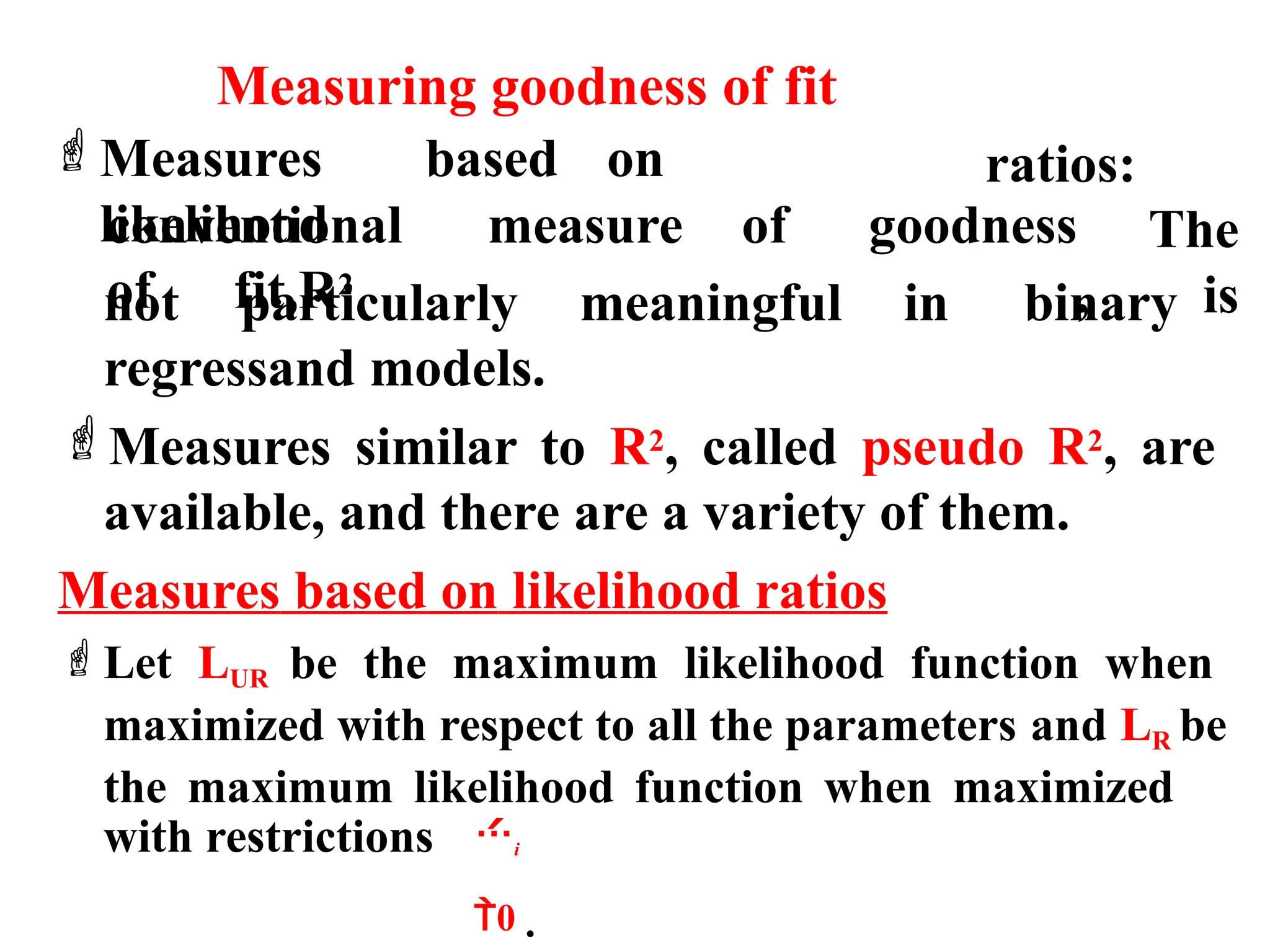
The document discusses the use of dummy variables in regression analysis, highlighting their role in quantifying qualitative characteristics like sex and race. It explains how these binary variables can illustrate differences in dependent variables such as salaries, alongside the classical assumptions of linear regression. Additionally, it details methods for determining the number of dummy variables needed when dealing with multiple categories and the implications of including interaction effects in models.


![The stages in running the Chow test are:
1. Run 2 separate regressions (say, before & after war
or policy reform, …) & save RSS's: RSS1 & RSS2.
RSS1 has n1–(K+1) df & RSS2 has n2–(K+1) df.
RSS1 + RSS2 = URSS with n1+n2–2(K+1) df.
2. Estimate pooled model (under H0: β's are stable).
RSS from this model is RRSS with n–(K+1)
df where n = n1+n2.
3. The test-statistic (under H0):
4. Find the critical value: FK+1,n-2(K+1) from table.
5. If Fcal>Ftab, reject H0 of stable parameters
(and favour Ha: there is structural break).
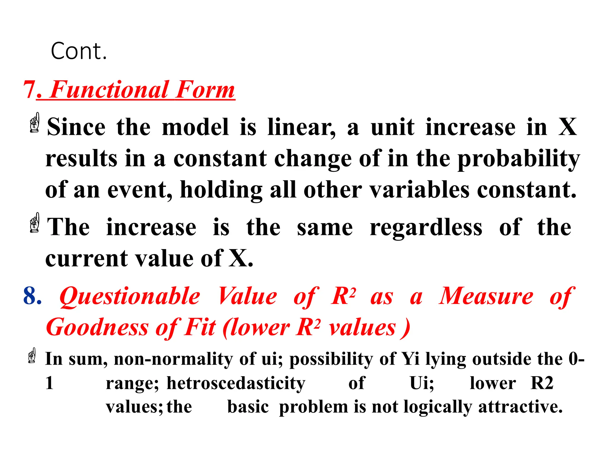
Cont.
U R S S
F
[ n 2 ( K 1 ) ]
[ R R S S U R S S ]
( K 1 )
c a l
76](https://image.slidesharecdn.com/presentation1-250110143431-406bd835/75/Presentation1-econometrics-2-by-habtamuu-76-2048.jpg)

![1. URSS = RSS1 + RSS2 = 15064.474
2. RRSS = 22064.6663
K = 1 and K + 1 = 2; n1 = 18, n2 = 15, n = 33.
3.
Thus,
4.ThetabulatedvaluefromtheF-distributionwith2 and29degreesof
freedomatthe5%levelof significanceis3.33.
5.Reject H0 at α=1%. Thus, there is structural break.
The pooled consumption model is an
inadequate specification; we should run separate
regressions.
The above method of calculating the Chow
test breaks down if either n1 < K+1 or n2 < K+1.
Solution: use Chow’s second (predictive) test!
29
15064.474
cal
[22064.6663 15064.474]
F 2 6.7632981
Cont.
78](https://image.slidesharecdn.com/presentation1-250110143431-406bd835/75/Presentation1-econometrics-2-by-habtamuu-78-2048.jpg)
![If, for instance, n2 < K+1, then the F-statistic will be
altered as follows:
One way of correcting for unequal 2 is to use
dummy variable regression with robust standard
errors.
RSS1
n2
1
n1 (K 1)
The Chow test tells if the parameters
differon average, but not which parameters
differ.
Also, it requires that all groups have the same 2.
This assumption is questionable: if parameters can
be different, then so can the variances be.
[RRSS RSS ]
Fcal
Cont.
79](https://image.slidesharecdn.com/presentation1-250110143431-406bd835/75/Presentation1-econometrics-2-by-habtamuu-79-2048.jpg)


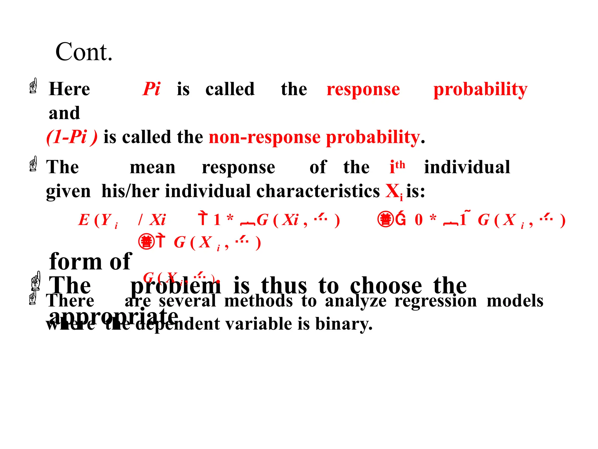
![Cont.
ith
The probability that the individual
chooses
alternative 1th (i.e. works) given his/
her individual characteristics, Xi is:
( measures the
impact of changes in X (say, age , marital status,
gender, education, occupation, and the like) on the
probability of labor force participation.
ith
The probability that the individual
chooses
i pr (Yi 1 / X i )
Pr[( U U 1
The vector of parameters
0 ] G ( X i ,
)
o
)
i
(1, 2 ,....,k )
alternative 0 (i.e. not to work) is given by:
pr(Y 0 / X ) 1 1 Pr[(U1
Uo
) 0] 1
G(X , )
i i i i i](https://image.slidesharecdn.com/presentation1-250110143431-406bd835/75/Presentation1-econometrics-2-by-habtamuu-88-2048.jpg)


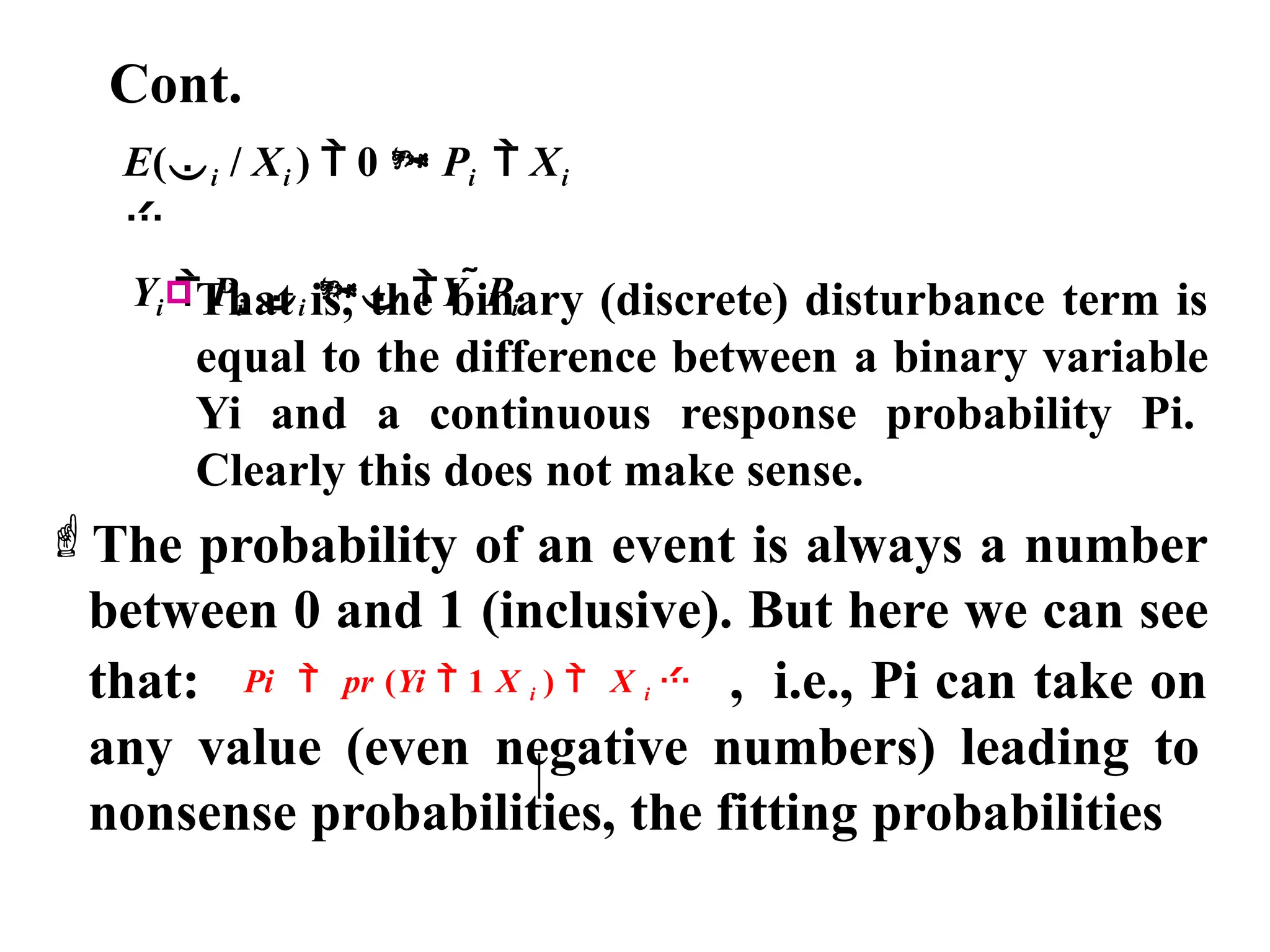
![Cont.
3. Error term assumes only two values.
If Yi=1 then i with the Probability,
Pi;
If Yi=0 then X with Probability, 1-Pi;
i i
The variance of the disturbance terms depends
on the X’s and is thus not constant.; i.e., error
term is not normally distributed.
Now by definition
since
E( i )
0by
assumption. Therefore, usingthe preceding
probability distribution of we obtain:
1 X i
Var(i ) [E( i E( i )]
E( )
2 2
i](https://image.slidesharecdn.com/presentation1-250110143431-406bd835/75/Presentation1-econometrics-2-by-habtamuu-97-2048.jpg)


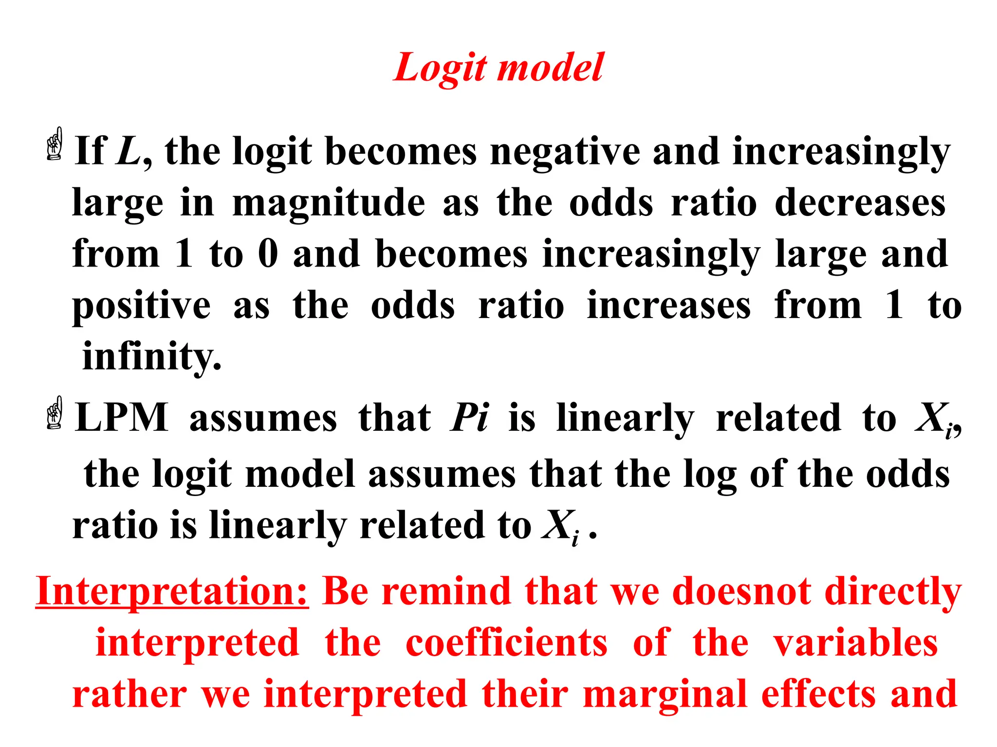
![Logit model
Various nonlinear functions have been
suggested for the function G in order to make
sure that the probabilities are between zero and
one.
In the logit model, G is the logistic function:
which is between zero and one for all real
numbers z. This is the cumulative distribution
function (cdf) for a standard logistic random
variable.
e X
1 e X
( z )
[1 exp( z )]
exp( z
)
G ( z )
](https://image.slidesharecdn.com/presentation1-250110143431-406bd835/75/Presentation1-econometrics-2-by-habtamuu-107-2048.jpg)
![Logit model
the response probability P(Y =1/X) is evaluated
as:
the non
response
probability P(Y =0/X)
is
evaluated as:
Note that: both response and non- response
probabilities lie in the interval [0 , 1] , and
hence, are interpretable.
Odd ratio: the ratio of the response probabilities
(Pi) to the non response probabilities (1-Pi).
1 e X
e
X
P P (Y 1 X )
eX
1
1 P P(Y 0 X) 1
1 eX
1 eX](https://image.slidesharecdn.com/presentation1-250110143431-406bd835/75/Presentation1-econometrics-2-by-habtamuu-108-2048.jpg)


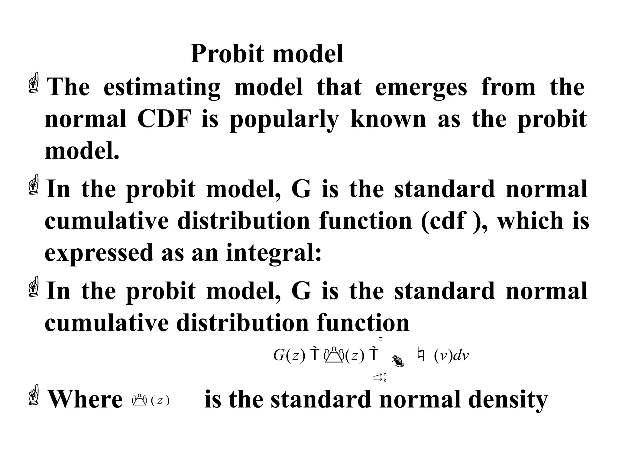
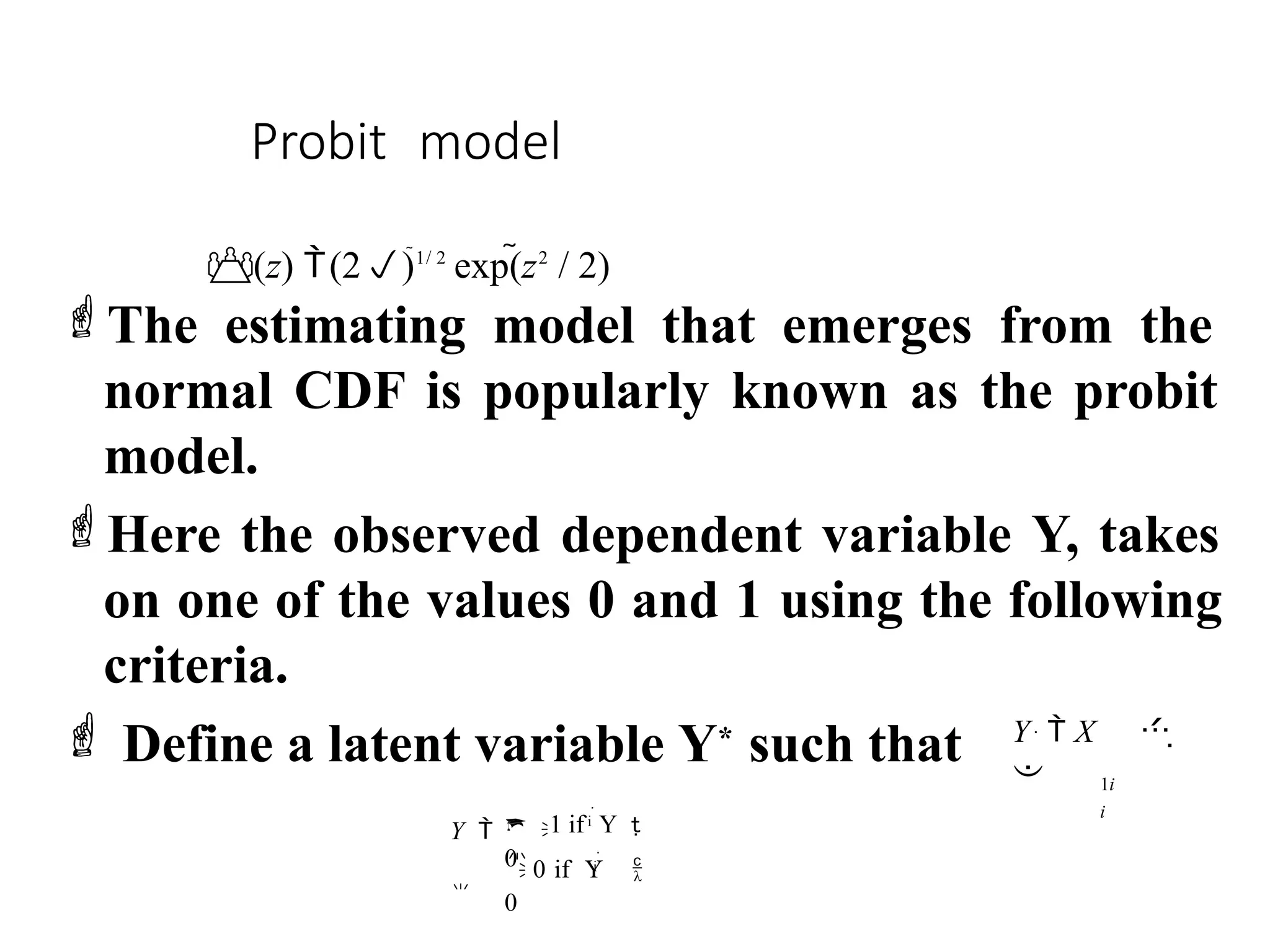
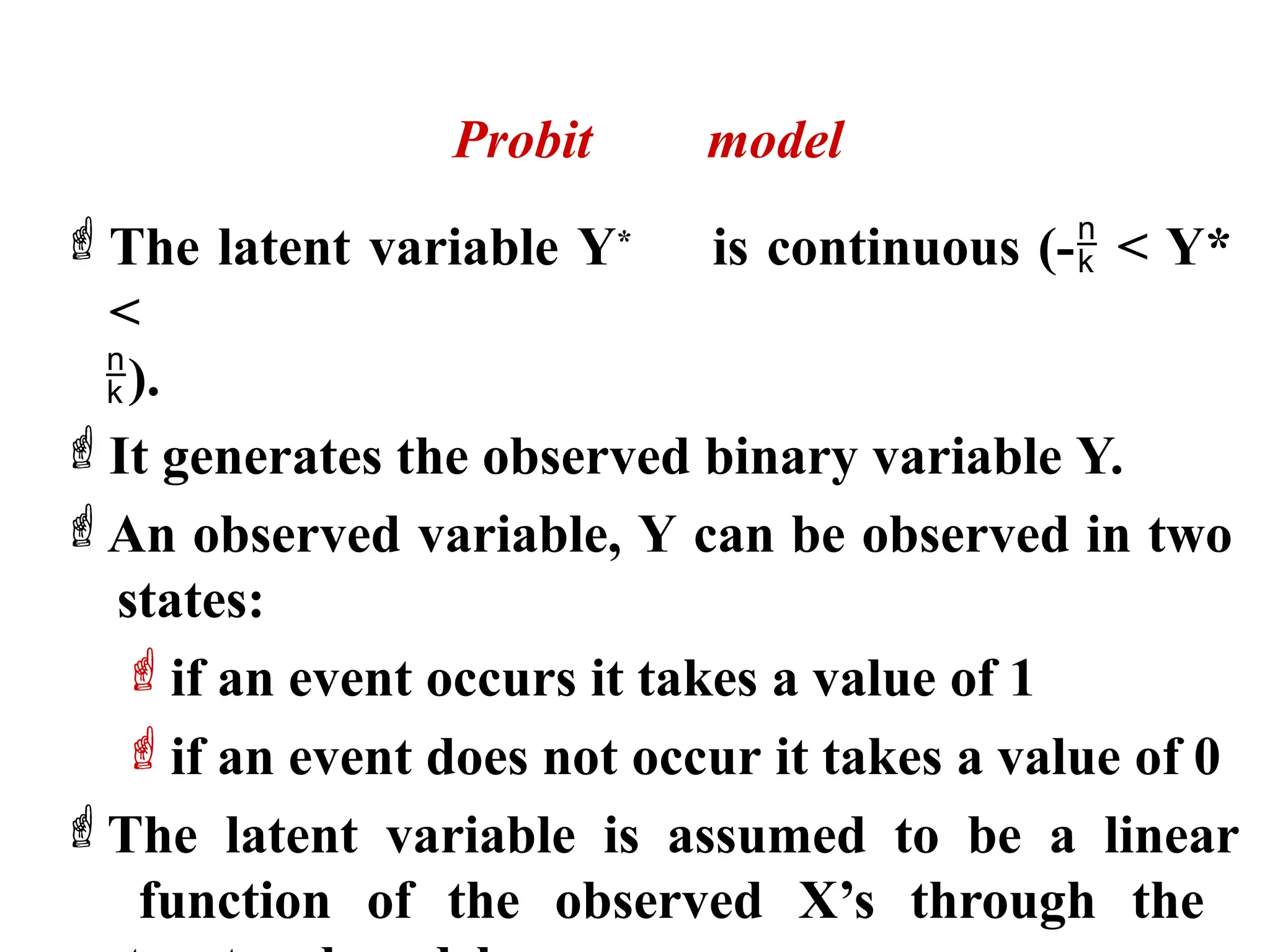

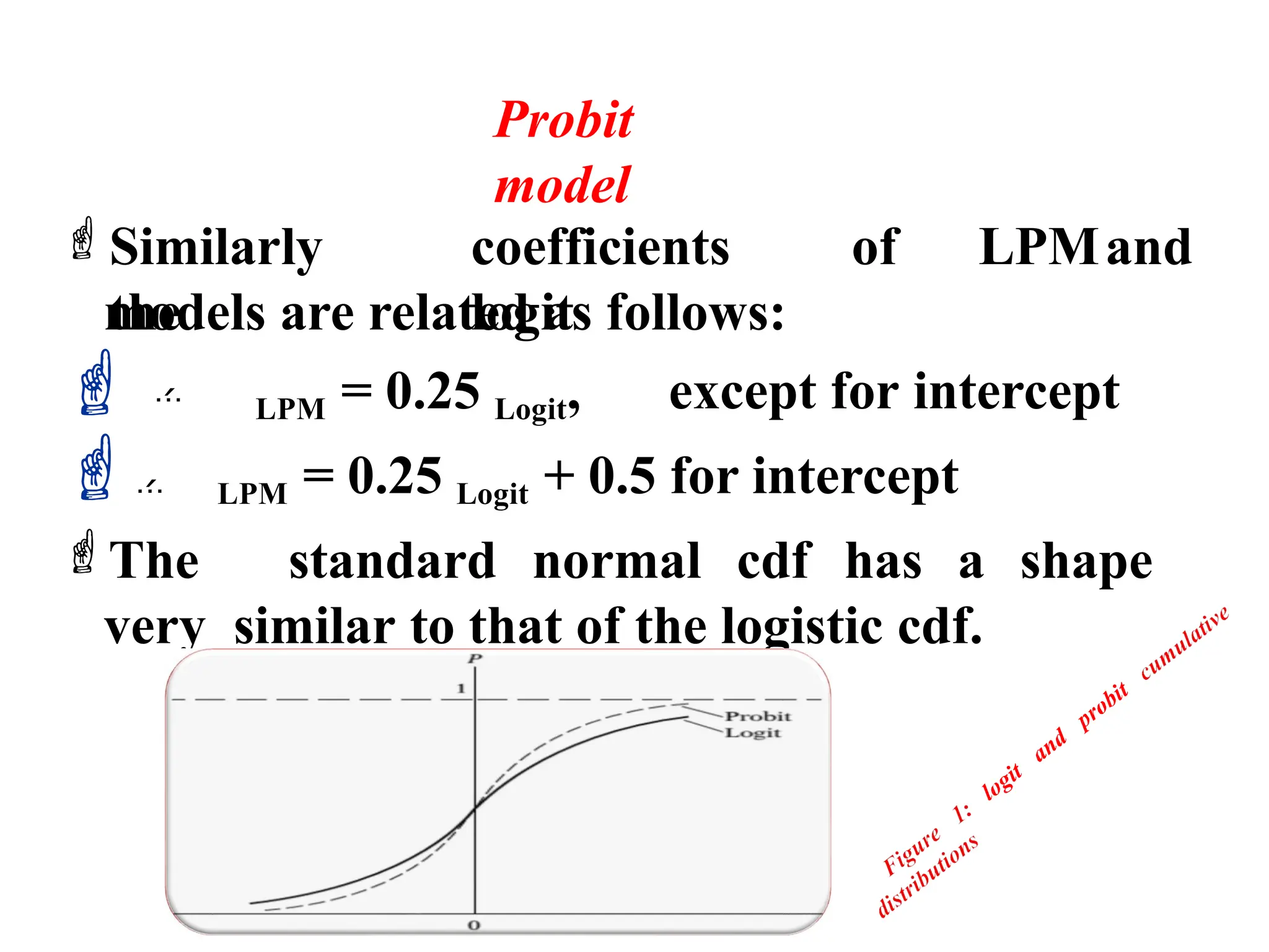
![Probit model
The coefficients derived from the maximum
likelihood (ML) function will be the coefficients
for the probit model, if we assume a normal
distribution.
If we assume that the appropriate distribution
of the error term is a logistic distribution, the
coefficients that we get from the ML function
will be the coefficient of the logit model.
In both cases, as with the LPM, it is assumed
that E[i/Xi] = 0](https://image.slidesharecdn.com/presentation1-250110143431-406bd835/75/Presentation1-econometrics-2-by-habtamuu-117-2048.jpg)