This document provides lecture notes on digital image processing. It discusses key topics such as the definition of digital images and how they are represented, the fundamental steps in digital image processing including image acquisition, enhancement, restoration, and compression, the components of an image processing system including sensors, hardware, software, storage and display, and elements of visual perception including the structure of the human eye and how light is sensed by the retina.


![Digital Image Processing
27
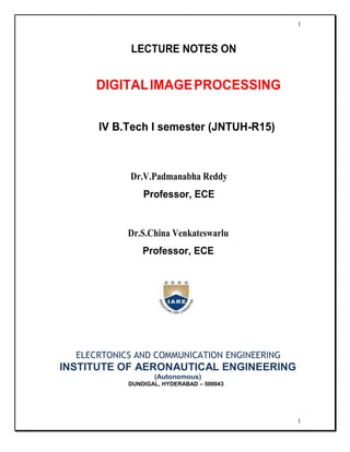
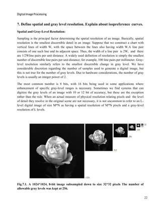
As a very rough rule of thumb, and assuming powers of 2 for convenience, images of size
256*256 pixels and 64 gray levels are about the smallest images that can be expected to be
reasonably free of objectionable sampling checker-boards and false contouring.
The results in Examples 7.2 and 7.3 illustrate the effects produced on image quality by varying N
and k independently. However, these results only partially answer the question of how varying N
and k affect images because we have not considered yet any relationships that might exist
between these two parameters.
An early study by Huang [1965] attempted to quantify experimentally the effects on image
quality produced by varying N and k simultaneously. The experiment consisted of a set of
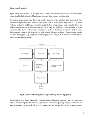
subjective tests. Images similar to those shown in Fig.7.4 were used. The woman’s face is
representative of an image with relatively little detail; the picture of the cameraman contains an
intermediate amount of detail; and the crowd picture contains, by comparison, a large amount of
detail. Sets of these three types of images were generated by varying N and k, and observers
were then asked to rank them according to their subjective quality. Results were summarized in
the form of so-called isopreference curves in the Nk-plane (Fig.7.5 shows average isopreference
curves representative of curves corresponding to the images shown in Fig. 7.4).Each point in the
Nk-plane represents an image having values of N and k equal to the coordinates of that point.
Fig.7.4 (a) Image with a low level of detail (b) Image with a medium level of detail (c) Image
with a relatively large amount of detail
Points lying on an isopreference curve correspond to images of equal subjective quality. It was
found in the course of the experiments that the isopreference curves tended to shift right and
upward, but their shapes in each of the three image categories were similar to those shown in](https://image.slidesharecdn.com/fzdjhosfqac3vchhf8as-dip-lecture-notes-230123055619-195b3297/85/DIP-LECTURE_NOTES-pdf-27-320.jpg)
![Digital Image Processing
29
8. Explain about Aliasing and Moire patterns.
Aliasing and Moiré Patterns:
Functions whose area under the curve is finite can be represented in terms of sines and cosines of
various frequencies. The sine/cosine component with the highest frequency determines the
highest ―frequency content‖ of the function. Suppose that this highest frequency is finite and that
the function is of unlimited duration (these functions are called band-limited functions).Then, the
Shannon sampling theorem [Brace well (1995)] tells us that, if the function is sampled at a rate
equal to or greater than twice its highest frequency, it is possible to recover completely the
original function from its samples. If the function is undersampled, then a phenomenon called
aliasing corrupts the sampled image. The corruption is in the form of additional frequency
components being introduced into the sampled function. These are called aliased frequencies.
Note that the sampling rate in images is the number of samples taken (in both spatial directions)
per unit distance.
As it turns out, except for a special case discussed in the following paragraph, it is impossible to
satisfy the sampling theorem in practice. We can only work with sampled data that are finite in
duration. We can model the process of converting a function of unlimited duration into a
function of finite duration simply by multiplying the unlimited function by a ―gating function‖
that is valued 1 for some interval and 0 elsewhere. Unfortunately, this function itself has
frequency components that extend to infinity. Thus, the very act of limiting the duration of a band-
limited function causes it to cease being band limited, which causes it to violate the key condition
of the sampling theorem. The principal approach for reducing the aliasing effects on an image is to
reduce its high-frequency components by blurring the image prior to sampling. However, aliasing
is always present in a sampled image. The effect of aliased frequencies can be seen under the right
conditions in the form of so called Moiré patterns.
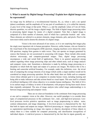
There is one special case of significant importance in which a function of infinite duration can be
sampled over a finite interval without violating the sampling theorem. When a function is
periodic, it may be sampled at a rate equal to or exceeding twice its highest frequency and it is
possible to recover the function from its samples provided that the sampling captures exactly an
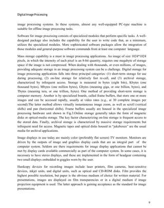
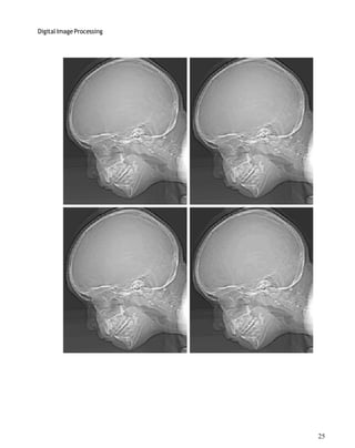
integer number of periods of the function. This special case allows us to illustrate vividly the
Moiré effect. Figure 8 shows two identical periodic patterns of equally spaced vertical bars,
rotated in opposite directions and then superimposed on each other by multiplying the two
images. A Moiré pattern, caused by a breakup of the periodicity, is seen in Fig.8 as a 2-D
sinusoidal (aliased) waveform (which looks like a corrugated tin roof) running in a vertical
direction. A similar pattern can appear when images are digitized (e.g., scanned) from a printed
page, which consists of periodic ink dots.](https://image.slidesharecdn.com/fzdjhosfqac3vchhf8as-dip-lecture-notes-230123055619-195b3297/85/DIP-LECTURE_NOTES-pdf-29-320.jpg)


![Digital Image Processing
42
F(u) = │F(u)│ejØ(u)
│F(u)│ = [R2
(u) + I2
(u)]1/2
Ø (u, v) = tan-1
[ I (u, v)/R (u, v) ]
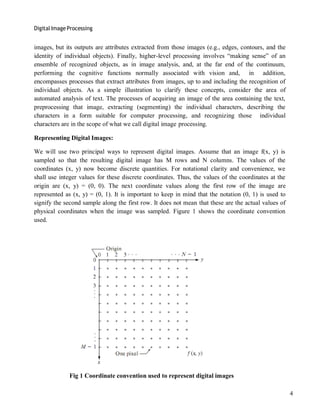
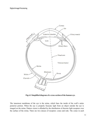
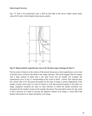
The magnitude function |F (u)| is called the Fourier Spectrum of f(x) and Φ(u) its phase angle.
The variable u appearing in the Fourier transform is called the frequency variable.
Fig 1 A simple function and its Fourier spectrum
The Fourier transform can be easily extended to a function f(x, y) of two variables. If f(x, y) is
continuous and integrable and F(u,v) is integrable, following Fourier transform pair exists
and
Where u, v are the frequency variables](https://image.slidesharecdn.com/fzdjhosfqac3vchhf8as-dip-lecture-notes-230123055619-195b3297/85/DIP-LECTURE_NOTES-pdf-42-320.jpg)
![Digital Image Processing
43
The Fourier spectrum, phase, are
│F(u, v)│ = [R2
(u, v) + I2
(u, v )]1/2
Ø(u, v) = tan-1
[ I(u, v)/R(u, v) ]
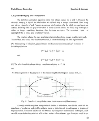
2. Define discrete Fourier transform and its inverse.
The discrete Fourier transform pair that applies to sampled function is given by,
(1)
For u = 0, 1, 2 . . . . , N-1, and
(2)
For x = 0, 1, 2 . . . ., N-1.
In the two variable case the discrete Fourier transform pair is
For u = 0, 1, 2 . . . , M-1, v = 0, 1, 2 . . . , N - 1, and
For x = 0, 1, 2 . . . , M-1, y = 0, 1, 2 . . . , N-1.
If M = N, then discrete Fourier transform pair is](https://image.slidesharecdn.com/fzdjhosfqac3vchhf8as-dip-lecture-notes-230123055619-195b3297/85/DIP-LECTURE_NOTES-pdf-43-320.jpg)
![Digital Image Processing
46
exp[j2Π(uox + voy)/N] = ejΠ(x + y)
=(-1)(x + y)](https://image.slidesharecdn.com/fzdjhosfqac3vchhf8as-dip-lecture-notes-230123055619-195b3297/85/DIP-LECTURE_NOTES-pdf-46-320.jpg)


![Digital Image Processing
52
For u = 0, 1, 2, . . , N-1. Similarly the inverse DCT is defined as
For u = 0, 1, 2, . . , N-1
Where α is
The corresponding 2-D DCT pair is
For u, v = 0, 1, 2, . . , N-1, and
For x, y= 0, 1, 2, . . , N-1
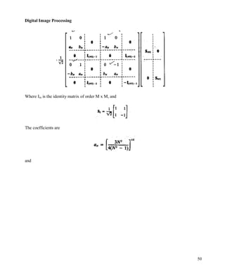
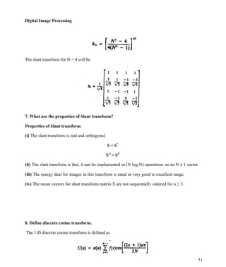
9. Explain about Haar transform.
The Haar transform is based on the Haar functions, hk(z), which are defined over the
continuous, closed interval z ε [0, 1], and for k = 0, 1, 2 . . . , N-1, where N = 2n
. The first step in
generating the Haar transform is to note that the integer k can be decomposed uniquely as
k = 2p
+ q - 1
where 0 ≤ p ≤ n-1, q = 0 or 1 for p = 0, and 1 ≤ q ≤ 2p
for p ≠ 0. For example, if N = 4, k, q, p
have following values](https://image.slidesharecdn.com/fzdjhosfqac3vchhf8as-dip-lecture-notes-230123055619-195b3297/85/DIP-LECTURE_NOTES-pdf-52-320.jpg)
![Digital Image Processing
53
The Haar functions are defined as
for z ε [0, 1] ……. (1)
and
These results allow derivation of Haar transformation matrices of order N x N by formation of
the ith row of a Haar matrix from elements oh hi(z) for z = 0/N, 1/N, . . . , (N-1)/N. For instance,
when N = 2, the first row of the 2 x 2 Haar matrix is computed by using ho(z) with z = 0/2, 1/2.
From equation (1) , ho(z) is equal to , independent of z, so the first row of the matrix has two
identical elements. Similarly row is computed. The 2 x 2 Haar matrix is
Similarly matrix for N = 4 is](https://image.slidesharecdn.com/fzdjhosfqac3vchhf8as-dip-lecture-notes-230123055619-195b3297/85/DIP-LECTURE_NOTES-pdf-53-320.jpg)


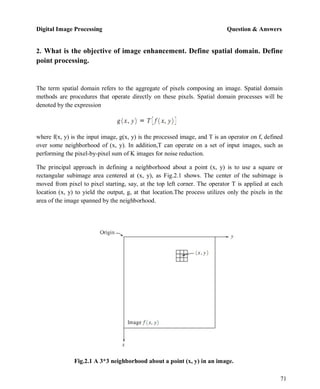
![Digital Image Processing Question & Answers
60
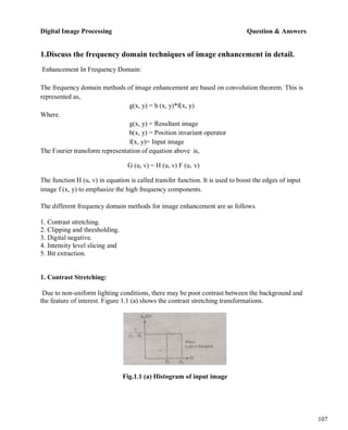
1.What is meant by image enhancement by point processing? Discuss any two
methods in it.
Basic Gray Level Transformations:
The study of image enhancement techniques is done by discussing gray-level transformation
functions. These are among the simplest of all image enhancement techniques. The values of
pixels, before and after processing, will be denoted by r and s, respectively. As indicated in the
previous section, these values are related by an expression of the form s=T(r), where T is a
transformation that maps a pixel value r into a pixel value s. Since we are dealing with digital
quantities, values of the transformation function typically are stored in a one-dimensional array
and the mappings from r to s are implemented via table lookups. For an 8-bit environment, a
lookup table containing the values of T will have 256 entries. As an introduction to gray-level
transformations, consider Fig. 1.1, which shows three basic types of functions used frequently
for image enhancement: linear (negative and identity transformations), logarithmic (log and
inverse-log transformations), and power-law (nth power and nth root transformations).The
identity function is the trivial case in which output intensities are identical to input intensities. It
is included in the graph only for completeness.
Image Negatives:
The negative of an image with gray levels in the range [0, L-1] is obtained by using the negative
transformation shown in Fig.1.1, which is given by the expression
s = L - 1 - r.
Reversing the intensity levels of an image in this manner produces the equivalent of a
photographic negative. This type of processing is particularly suited for enhancing white or gray
detail embedded in dark regions of an image, especially when the black areas are dominant in
size.](https://image.slidesharecdn.com/fzdjhosfqac3vchhf8as-dip-lecture-notes-230123055619-195b3297/85/DIP-LECTURE_NOTES-pdf-60-320.jpg)


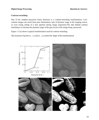
![Digital Image Processing Question & Answers
65
Fig.1.3 Contrast Stretching (a) Form of Transformation function (b) A low-contrast image
(c) Result of contrast stretching (d) Result of thresholding.
function. If r1=s1 and r2=s2, the transformation is a linear function that produces no changes in
gray levels. If r1=r2,s1=0 and s2=L-1, the transformation becomes a thresholding function that
creates a binary image, as illustrated in Fig. 1.3 (b). Intermediate values of (r1 , s1) and (r2 , s2)
produce various degrees of spread in the gray levels of the output image, thus affecting its
contrast. In general, r1 ≤ r2 and s1 ≤ s2 is assumed so that the function is single valued and
monotonically increasing.This condition preserves the order of gray levels, thus preventing the
creation of intensity artifacts in the processed image.
Figure 1.3 (b) shows an 8-bit image with low contrast. Fig. 1.3(c) shows the result of contrast
stretching, obtained by setting (r1 , s1) = (rmin , 0) and (r2 , s2) = (rmax , L-1) where rmin and rmax
denote the minimum and maximum gray levels in the image, respectively.Thus, the
transformation function stretched the levels linearly from their original range to the full range [0,
L-1]. Finally, Fig. 1.3 (d) shows the result of using the thresholding function defined
previously,with r1 = r2 = m, the mean gray level in the image.The original image on which these
results are based is a scanning electron microscope image of pollen,magnified approximately 700
times.
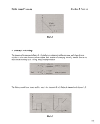
Gray-level slicing:
Highlighting a specific range of gray levels in an image often is desired. Applications include
enhancing features such as masses of water in satellite imagery and enhancing flaws in X-ray
images.There are several ways of doing level slicing, but most of them are variations of two
basic themes.One approach is to display a high value for all gray levels in the range of interest
and a low value for all other gray levels.This transformation, shown in Fig. 1.4 (a), produces a
binary image.The second approach, based on the transformation shown in Fig. 1.4 (b), brightens
the desired range of gray levels but preserves the background and gray-level tonalities in the
image. Figure 1.4(c) shows a gray-scale image, and Fig. 1.4 (d) shows the result of using the
transformation in Fig. 1.4 (a).Variations of the two transformations shown in Fig. 1.4 are easy to
formulate.](https://image.slidesharecdn.com/fzdjhosfqac3vchhf8as-dip-lecture-notes-230123055619-195b3297/85/DIP-LECTURE_NOTES-pdf-65-320.jpg)
![Digital Image Processing Question & Answers
66
Fig.1.4 (a) This transformation highlights range [A, B] of gray levels and reduce all others
to a constant level (b) This transformation highlights range [A, B] but preserves all other
levels (c) An image (d) Result of using the transformation in (a).
Bit-plane slicing:
Instead of highlighting gray-level ranges, highlighting the contributionmade to total image
appearance by specific bits might be desired. Suppose that each pixel in an image is represented
by 8 bits. Imagine that the image is composed of eight 1-bit planes, ranging from bit-plane 0 for](https://image.slidesharecdn.com/fzdjhosfqac3vchhf8as-dip-lecture-notes-230123055619-195b3297/85/DIP-LECTURE_NOTES-pdf-66-320.jpg)


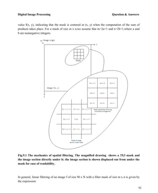
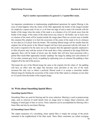
![Digital Image Processing Question & Answers
74
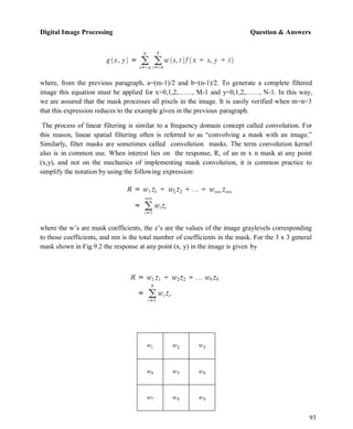
(also referred to as filters, kernels, templates, or windows). Basically, a mask is a small (say,
3*3) 2-D array, such as the one shown in Fig. 2.1, in which the values of the mask coefficients
determine the nature of the process, such as image sharpening.
3. Define histogram of a digital image. Explain how histogram is useful in
image enhancement?
Histogram Processing:
The histogram of a digital image with gray levels in the range [0, L-1] is a discrete function h(rk)
= (nk), where rk is the kth gray level and nk is the number of pixels in the image having gray level
rk. It is common practice to normalize a histogram by dividing each of its values by the total
number of pixels in the image, denoted by n. Thus, a normalized histogram is given by
for k=0,1,…… .,L-1. Loosely speaking, p(rk) gives an estimate of the probability of occurrence
of gray level rk. Note that the sum of all components of a normalized histogram is equal to 1.
Histograms are the basis for numerous spatial domain processing techniques.Histogram
manipulation can be used effectively for image enhancement. Histograms are simple to calculate
in software and also lend themselves to economic hardware implementations, thus making them
a popular tool for real-time image processing.
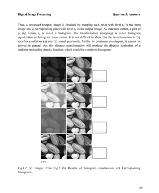
As an introduction to the role of histogram processing in image enhancement, consider Fig. 3,
which is the pollen image shown in four basic gray-level characteristics: dark, light, low contrast,
and high contrast.The right side of the figure shows the histograms corresponding to these
images. The horizontal axis of each histogram plot corresponds to gray level values, rk.
The vertical axis corresponds to values of h(rk) = nk or p(rk) = nk/n if the values are
normalized.Thus, as indicated previously, these histogram plots are simply plots of h(rk) = nk
versus rk or p(rk) = nk/n versus rk.](https://image.slidesharecdn.com/fzdjhosfqac3vchhf8as-dip-lecture-notes-230123055619-195b3297/85/DIP-LECTURE_NOTES-pdf-74-320.jpg)


![Digital Image Processing Question & Answers
77
range. It will be shown shortly that it is possible to develop a transformation function that can
automatically achieve this effect, based only on information available in the histogram of the
input image.
4. Write about histogram equalization.
Histogram Equalization:
Consider for a moment continuous functions, and let the variable r represent the gray levels of
the image to be enhanced. We assume that r has been normalized to the interval [0, 1], with r=0
representing black and r=1 representing white. Later, we consider a discrete formulation and
allow pixel values to be in the interval [0, L-1]. For any r satisfying the aforementioned
conditions, we focus attention on transformations of the form
that produce a level s for every pixel value r in the original image. For reasons that will become
obvious shortly, we assume that the transformation function T(r) satisfies the following
conditions:
(a) T(r) is single-valued and monotonically increasing in the interval 0 ≤ r ≤ 1; and
(b) 0 ≤ T(r) ≤ 1 for 0 ≤ r ≤ 1.
The requirement in (a) that T(r) be single valued is needed to guarantee that the inverse
transformation will exist, and the monotonicity condition preserves the increasing order from
black to white in the output image.A transformation function that is not monotonically increasing
could result in at least a section of the intensity range being inverted, thus producing some
inverted gray levels in the output image. Finally, condition (b) guarantees that the output gray
levels will be in the same range as the input levels. Figure 4.1 gives an example of a
transformation function that satisfies these two conditions.The inverse transformation from s
back to r is denoted
It can be shown by example that even if T(r) satisfies conditions (a) and (b), it is possible that the
corresponding inverse T-1
(s) may fail to be single valued.](https://image.slidesharecdn.com/fzdjhosfqac3vchhf8as-dip-lecture-notes-230123055619-195b3297/85/DIP-LECTURE_NOTES-pdf-77-320.jpg)
![Digital Image Processing Question & Answers
78
.
Fig.4.1 A gray-level transformation function that is both single valued and monotonically
increasing.
The gray levels in an image may be viewed as random variables in the interval [0, 1].One of the
most fundamental descriptors of a random variable is its probability density function (PDF).Let
pr(r) and ps(s) denote the probability density functions of random variables r and s,
respectively,where the subscripts on p are used to denote that pr and ps are different functions.A
basic result from an elementary probability theory is that, if pr(r) and T(r) are known and T-1
(s)
satisfies condition (a), then the probability density function ps(s) of the transformed variable s
can be obtained using a rather simple formula:
Thus, the probability density function of the transformed variable, s, is determined by the gray-
level PDF of the input image and by the chosen transformation function. A transformation
function of particular importance in image processing has the form
where w is a dummy variable of integration.The right side of Eq. above is recognized as the
cumulative distribution function (CDF) of random variable r. Since probability density functions
are always positive, and recalling that the integral of a function is the area under the function, it
follows that this transformation function is single valued and monotonically increasing, and,
therefore, satisfies condition (a). Similarly, the integral of a probability density function for
variables in the range [0, 1] also is in the range [0, 1], so condition (b) is satisfied as well.](https://image.slidesharecdn.com/fzdjhosfqac3vchhf8as-dip-lecture-notes-230123055619-195b3297/85/DIP-LECTURE_NOTES-pdf-78-320.jpg)
![Digital Image Processing Question & Answers
79
Given transformation function T(r),we find ps(s) by applying Eq. We know from basic calculus
(Leibniz’s rule) that the derivative of a definite integral with respect to its upper limit is simply
the integrand evaluated at that limit. In other words,
Substituting this result for dr/ds, and keeping in mind that all probability values are positive,
yields
Because ps(s) is a probability density function, it follows that it must be zero outside the interval
[0, 1] in this case because its integral over all values of s must equal 1.We recognize the form of
ps(s) as a uniform probability density function. Simply stated, we have demonstrated that
performing the transformation function yields a random variable s characterized by a uniform
probability density function. It is important to note from Eq. discussed above that T(r) depends
on pr(r), but, as indicated by Eq. after it, the resulting ps(s) always is uniform, independent of the
form of pr(r). For discrete values we deal with probabilities and summations instead of
probability density functions and integrals. The probability of occurrence of gray level r in an
image is approximated by
where, as noted at the beginning of this section, n is the total number of pixels in the image, nk is
the number of pixels that have gray level rk, and L is the total number of possible gray levels in
the image.The discrete version of the transformation function given in Eq. is](https://image.slidesharecdn.com/fzdjhosfqac3vchhf8as-dip-lecture-notes-230123055619-195b3297/85/DIP-LECTURE_NOTES-pdf-79-320.jpg)


![Digital Image Processing Question & Answers
83
As in the continuos case, we are seeking values of z that satisfy this equation.The variable vk was
added here for clarity in the discussion that follows. Finally, the discrete version of the above
Eqn. is given by
Or
Implementation:
We start by noting the following: (1) Each set of gray levels {rj} , {sj}, and {zj}, j=0, 1, 2, p , L-
1, is a one-dimensional array of dimension L X 1. (2) All mappings from r to s and from s to z
are simple table lookups between a given pixel value and these arrays. (3) Each of the elements
of these arrays, for example, sk, contains two important pieces of information: The subscript k
denotes the location of the element in the array, and s denotes the value at that location. (4) We
need to be concerned only with integer pixel values. For example, in the case of an 8-bit image,
L=256 and the elements of each of the arrays just mentioned are integers between 0 and 255.This
implies that we now work with gray level values in the interval [0, L-1] instead of the normalized
interval [0, 1] that we used before to simplify the development of histogram processing
techniques.
In order to see how histogram matching actually can be implemented, consider Fig. 5(a),
ignoring for a moment the connection shown between this figure and Fig. 5(c). Figure 5(a)
shows a hypothetical discrete transformation function s=T(r) obtained from a given image. The
first gray level in the image, r1 , maps to s1 ; the second gray level, r2 , maps to s2 ; the kth level rk
maps to sk; and so on (the important point here is the ordered correspondence between these
values). Each value sj in the array is precomputed, so the process of mapping simply uses the
actual value of a pixel as an index in an array to determine the corresponding value of s.This
process is particularly easy because we are dealing with integers. For example, the s mapping for
an 8-bit pixel with value 127 would be found in the 128th position in array {sj} (recall that we
start at 0) out of the possible 256 positions. If we stopped here and mapped the value of each
pixel of an input image by the](https://image.slidesharecdn.com/fzdjhosfqac3vchhf8as-dip-lecture-notes-230123055619-195b3297/85/DIP-LECTURE_NOTES-pdf-83-320.jpg)

![Digital Image Processing Question & Answers
85
Since we really do not have the z’s (recall that finding these values is precisely the objective of
histogram matching),we must resort to some sort of iterative scheme to find z from s.The fact
that we are dealing with integers makes this a particularly simple process. Basically, because vk =
sk, we have that the z’s for which we are looking must satisfy the equation G(zk)=sk, or (G(zk)-
sk)=0. Thus, all we have to do to find the value of zk corresponding to sk is to iterate on values of
z such that this equation is satisfied for k=0,1,2,…...., L-1. We do not have to find the inverse of
G because we are going to iterate on z. Since we are dealing with integers, the closest we can get
to satisfying the equation (G(zk)-sk)=0 is to let zk= for each value of k, where is the
smallest integer in the interval [0, L-1] such that
Given a value sk, all this means conceptually in terms of Fig. 5(c) is that we would start with and
increase it in integer steps until Eq is satisfied, at which point we let repeating this process for
all values of k would yield all the required mappings from s to z, which constitutes the
implementation of Eq. In practice, we would not have to start with each time because the values
of sk are known to increase monotonically. Thus, for k=k+1, we would start with and
increment in integer values from there.
6. Write about Local enhancement.
Local Enhancement:
The histogram processing methods discussed in the previous two sections are global, in the sense
that pixels are modified by a transformation function based on the gray-level content of an entire
image. Although this global approach is suitable for overall enhancement, there are cases in
which it is necessary to enhance details over small areas in an image. The number of pixels in
these areas may have negligible influence on the computation of a global transformation whose
shape does not necessarily guarantee the desired local enhancement. The solution is to devise
transformation functions based on the gray-level distribution—or other properties—in the
neighborhood of every pixel in the image.
The histogram processing techniques are easily adaptable to
local enhancement.The procedure is to define a square or rectangular neighborhood and move
the center of this area from pixel to pixel. At each location, the histogram of the points in the
neighborhood is computed and either a histogram equalization or histogram specification](https://image.slidesharecdn.com/fzdjhosfqac3vchhf8as-dip-lecture-notes-230123055619-195b3297/85/DIP-LECTURE_NOTES-pdf-85-320.jpg)


![Digital Image Processing Question & Answers
99
assign this value to that pixel. For example, in a 3 x 3 neighborhood the median is the 5th largest
value, in a 5 x 5 neighborhood the 13th largest value, and so on. When several values in a
neighborhood are the same, all equal values are grouped. For example, suppose that a 3 x 3
neighborhood has values (10, 20, 20, 20, 15, 20, 20, 25, 100). These values are sorted as (10, 15,
20, 20, 20, 20, 20, 25, 100), which results in a median of 20. Thus, the principal function of
median filters is to force points with distinct gray levels to be more like their neighbors. In fact,
isolated clusters of pixels that are light or dark with respect to their neighbors, and whose area is
less than n2 /
2 (one-half the filter area), are eliminated by an n x n median filter. In this case
―eliminated‖ means forced to the median intensity of the neighbors. Larger clusters are affected
considerably less.
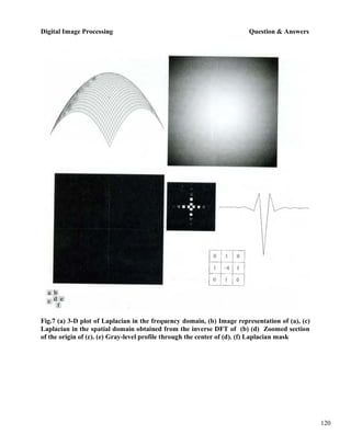
11. What is meant by the Gradiant and the Laplacian? Discuss their role in
image enhancement.
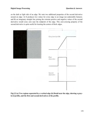
Use of Second Derivatives for Enhancement–The Laplacian:
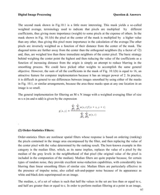
The approach basically consists of defining a discrete formulation of the second-order derivative
and then constructing a filter mask based on that formulation. We are interested in isotropic
filters, whose response is independent of the direction of the discontinuities in the image to
which the filter is applied. In other words, isotropic filters are rotation invariant, in the sense that
rotating the image and then applying the filter gives the same result as applying the filter to the
image first and then rotating the result.
Development of the method:
It can be shown (Rosenfeld and Kak [1982]) that the simplest isotropic derivative operator is the
Laplacian, which, for a function (image) f(x, y) of two variables, is defined as
Because derivatives of any order are linear operations, the Laplacian is a linear operator. In order
to be useful for digital image processing, this equation needs to be expressed in discrete form.
There are several ways to define a digital Laplacian using neighborhoods. digital second.Taking
into account that we now have two variables, we use the following notation for the partial second-](https://image.slidesharecdn.com/fzdjhosfqac3vchhf8as-dip-lecture-notes-230123055619-195b3297/85/DIP-LECTURE_NOTES-pdf-99-320.jpg)


![Digital Image Processing Question & Answers
104
The computational burden of implementing over an entire image is not trivial, and it is common
practice to approximate the magnitude of the gradient by using absolute values instead of squares
and square roots:
This equation is simpler to compute and it still preserves relative changes in gray levels, but the
isotropic feature property is lost in general. However, as in the case of the Laplacian, the
isotropic properties of the digital gradient defined in the following paragraph are preserved only
for a limited number of rotational increments that depend on the masks used to approximate the
derivatives. As it turns out, the most popular masks used to approximate the gradient give the
same result only for vertical and horizontal edges and thus the isotropic properties of the gradient
are preserved only for multiples of 90°.
As in the case of the Laplacian, we now define digital
approximations to the preceding equations, and from there formulate the appropriate filter masks.
In order to simplify the discussion that follows, we will use the notation in Fig. 11.2 (a) to denote
image points in a 3 x 3 region. For example, the center point, z5 , denotes f(x, y), z1 denotes f(x-
1, y-1), and so on. The simplest approximations to a first-order derivative that satisfy the
conditions stated in that section are Gx = (z8 –z5) and Gy = (z6 – z5) . Two other definitions
proposed by Roberts [1965] in the early development of digital image processing use cross
differences:
we compute the gradient as
If we use absolute values, then substituting the quantities in the equations gives us the following
approximation to the gradient:
This equation can be implemented with the two masks shown in Figs. 11.2 (b) and(c). These
masks are referred to as the Roberts cross-gradient operators. Masks of even size are awkward to
implement. The smallest filter mask in which we are interested is of size 3 x 3.An approximation
using absolute values, still at point z5 , but using a 3*3 mask, is](https://image.slidesharecdn.com/fzdjhosfqac3vchhf8as-dip-lecture-notes-230123055619-195b3297/85/DIP-LECTURE_NOTES-pdf-104-320.jpg)


![Digital Image Processing Question & Answers
108
Fig.1.1 (b) Linear Law
Fig.1.1 (c) Histogram of the transformed image
These stretching transformations are expressed as
In the area of stretching the slope of transformation is considered to be greater than unity. The
parameters of stretching transformations i.e., a and b can be determined by examining the
histogram of the image.
2. Clipping and Thresholding:
Clipping is considered as the special scenario of contrast stretching. It is the case in which the
parameters are α = γ = 0. Clipping is more advantageous for reduction of noise in input signals of
range [a, b].
Threshold of an image is selected by means of its histogram. Let us take the image shown in the
following figure 1.2.](https://image.slidesharecdn.com/fzdjhosfqac3vchhf8as-dip-lecture-notes-230123055619-195b3297/85/DIP-LECTURE_NOTES-pdf-108-320.jpg)

![Digital Image Processing Question & Answers
111
When an image is uniformly quantized then, the nth
most significant bit can be extracted and
displayed.
Let, u = k1 2B-1
+ k2 2B-2
+……………..+ kB-1 2 + kB
Then, the output is expressed as
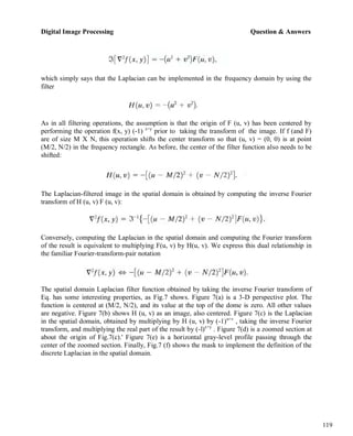
2. Distinguish between spatial domain and frequency domain enhancement
techniques.
The spatial domain refers to the image plane itself, and approaches in this category are based on
direct manipulation of pixels in an image. Frequency domain processing techniques are based on
modifying the Fourier transform of an image.
The term spatial domain refers to the aggregate of pixels
composing an image and spatial domain methods are procedures that operate directly on these
pixels. Image processing function in the spatial domain may he expressed as.
g(x, y) = T[f(x, y)]
Where
(x, y).
f(x, y) is the input image
g(x, y) is the processed image and
T is the operator on f defined over some neighborhood values of
Frequency domain techniques are based on convolution theorem. Let g(x, y) be the image
formed by the convolution of an image f(x, y) and linear position invariant operation h(x, y) i.e.,
g(x, y) = h(x, y) * f(x, y)
Applying convolution theorem
G(u, v) = H(u, v) F(u, v)](https://image.slidesharecdn.com/fzdjhosfqac3vchhf8as-dip-lecture-notes-230123055619-195b3297/85/DIP-LECTURE_NOTES-pdf-111-320.jpg)


![Digital Image Processing Question & Answers
129
where we used the fact that the product of a complex quantity with its conjugate is equal to the
magnitude of the complex quantity squared. This result is known as the Wiener filter, after N.
Wiener [1942], who first proposed the concept in the year shown. The filter, which consists of
the terms inside the brackets, also is commonly referred to as the minimum mean square error
filter or the least square error filter. The Wiener filter does not have the same problem as the
inverse filter with zeros in the degradation function, unless both H(u, v) and Sη(u, v) are zero for
the same value(s) of u and v.
The terms in above equation are as follows:
H (u, v) = degradation function
H*(u, v) = complex conjugate of H (u, v)
│H (u, v│ 2
= H*(u, v)* H (u, v)
Sη (u, v) = │N (u, v) 2
= power spectrum of the noise
Sf (u, v) = │F (u, v) 2
= power spectrum of the undegraded image.
As before, H (u, v) is the transform of the degradation function and G (u, v) is the
transform of the degraded image. The restored image in the spatial domain is given by the
inverse Fourier transform of the frequency-domain estimate F (u, v). Note that if the noise is
zero, then the noise power spectrum vanishes and the Wiener filter reduces to the inverse filter.
When we are dealing with spectrally white noise, the spectrum │N (u, v│ 2
is a constant,
which simplifies things considerably. However, the power spectrum of the undegraded image
seldom is known. An approach used frequently when these quantities are not known or cannot be
estimated is to approximate the equation as](https://image.slidesharecdn.com/fzdjhosfqac3vchhf8as-dip-lecture-notes-230123055619-195b3297/85/DIP-LECTURE_NOTES-pdf-129-320.jpg)


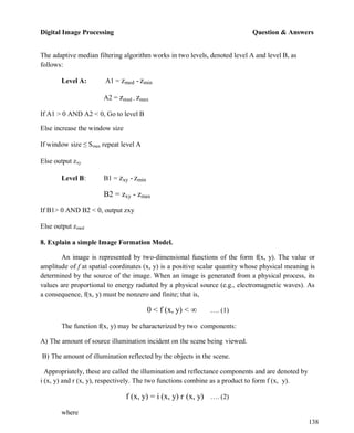
![Digital Image Processing Question & Answers
139
and
0 < i (x, y) < ∞ …. (3)
0 < r (x, y) < 1 …. (4)
Equation (4) indicates that reflectance is bounded by 0 (total absorption) and 1 (total
reflectance).The nature of i (x, y) is determined by the illumination source, and r (x, y) is
determined by the characteristics of the imaged objects. It is noted that these expressions also are
applicable to images formed via transmission of the illumination through a medium, such as a
chest X-ray.
9. Write brief notes on inverse filtering.
The simplest approach to restoration is direct inverse filtering, where F (u, v), the
transform of the original image is computed simply by dividing the transform of the degraded
image, G (u, v), by the degradation function
The divisions are between individual elements of the functions.
But G (u, v) is given by
Hence
G (u, v) = F (u, v) + N (u, v)
It tells that even if the degradation function is known the undegraded image cannot be
recovered [the inverse Fourier transform of F( u, v)] exactly because N(u, v) is a random
function whose Fourier transform is not known.
If the degradation has zero or very small values, then the ratio N(u, v)/H(u, v) could
easily dominate the estimate F(u, v).
One approach to get around the zero or small-value problem is to limit the filter](https://image.slidesharecdn.com/fzdjhosfqac3vchhf8as-dip-lecture-notes-230123055619-195b3297/85/DIP-LECTURE_NOTES-pdf-139-320.jpg)

![Digital Image Processing Question & Answers
141
is usually the highest value of H (u, v) in the frequency domain. Thus, by limiting the analysis to
frequencies near the origin, the probability of encountering zero values is reduced.
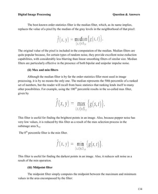
10. Write about Noise Probability Density Functions.
The following are among the most common PDFs found in image processing applications.
Gaussian noise
Because of its mathematical tractability in both the spatial and frequency domains,
Gaussian (also called normal) noise models are used frequently in practice. In fact, this
tractability is so convenient that it often results in Gaussian models being used in situations in
which they are marginally applicable at best.
The PDF of a Gaussian random variable, z, is given by
… (1)
where z represents gray level, µ is the mean of average value of z, and a σ is its standard
deviation. The standard deviation squared, σ2
, is called the variance of z. A plot of this function
is shown in Fig. 5.10. When z is described by Eq. (1), approximately 70% of its values will be in
the range [(µ - σ), (µ +σ)], and about 95% will be in the range [(µ - 2σ), (µ + 2σ)].
Rayleigh noise
The PDF of Rayleigh noise is given by
The mean and variance of this density are given by
µ = a +ƒMb/4
σ2
= b(4 – Π)/4](https://image.slidesharecdn.com/fzdjhosfqac3vchhf8as-dip-lecture-notes-230123055619-195b3297/85/DIP-LECTURE_NOTES-pdf-141-320.jpg)


![Digital Image Processing Question & Answers
161
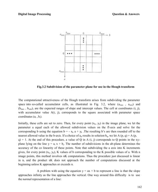
(ii) Global processing via the Hough Transform:
In this process, points are linked by determining first if they lie on a curve of specified shape. We
now consider global relationships between pixels. Given n points in an image, suppose that we
want to find subsets of these points that lie on straight lines. One possible solution is to first find
all lines determined by every pair of points and then find all subsets of points that are close to
particular lines. The problem with this procedure is that it involves finding n(n - 1)/2 ~ n2
lines
and then performing (n)(n(n - l))/2 ~ n3
comparisons of every point to all lines. This approach is
computationally prohibitive in all but the most trivial applications.
Hough [1962] proposed an alternative approach, commonly referred to as the Hough transform.
Consider a point (xi, yi) and the general equation of a straight line in slope-intercept form,
yi = a.xi + b. Infinitely many lines pass through (xi, yi) but they all satisfy the equation
yi = a.xi + b for varying values of a and b. However, writing this equation as b = -a.xi + yi, and
considering the ab-plane (also called parameter space) yields the equation of a single line for a
fixed pair (xi, yi). Furthermore, a second point (xj, yj) also has a line in parameter space
associated with it, and this line intersects the line associated with (xi, yi) at (a', b'), where a' is the
slope and b' the intercept of the line containing both (xi, yi) and (xj, yj) in the xy-plane. In fact, all
points contained on this line have lines in parameter space that intersect at (a', b'). Figure 3.1
illustrates these concepts.
Fig.3.1 (a) xy-plane (b) Parameter space](https://image.slidesharecdn.com/fzdjhosfqac3vchhf8as-dip-lecture-notes-230123055619-195b3297/85/DIP-LECTURE_NOTES-pdf-161-320.jpg)


![Digital Image Processing Question & Answers
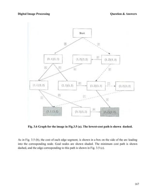
166
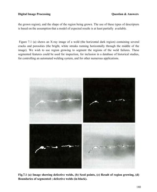
Fig.3.5 (a) A 3 X 3 image region, (b) Edge segments and their costs, (c) Edge corresponding
to the lowest-cost path in the graph shown in Fig. 3.6
coordinates and the numbers in brackets represent gray-level values. Each edge element, defined
by pixels p and q, has an associated cost, defined as
where H is the highest gray-level value in the image (7 in this case), and f(p) and f(q) are the gray-
level values of p and q, respectively. By convention, the point p is on the right-hand side of the
direction of travel along edge elements. For example, the edge segment (1, 2) (2, 2) is between
points (1, 2) and (2, 2) in Fig. 3.5 (b). If the direction of travel is to the right, then p is the point
with coordinates (2, 2) and q is point with coordinates (1, 2); therefore, c (p, q) = 7 - [7
- 6] = 6. This cost is shown in the box below the edge segment. If, on the other hand, we are
traveling to the left between the same two points, then p is point (1, 2) and q is (2, 2). In this case
the cost is 8, as shown above the edge segment in Fig. 3.5(b). To simplify the discussion, we
assume that edges start in the top row and terminate in the last row, so that the first element of an
edge can be only between points (1, 1), (1, 2) or (1, 2), (1, 3). Similarly, the last edge element has
to be between points (3, 1), (3, 2) or (3, 2), (3, 3). Keep in mind that p and q are 4-neighbors, as
noted earlier. Figure 3.6 shows the graph for this problem. Each node (rectangle) in the graph
corresponds to an edge element from Fig. 3.5. An arc exists between two nodes if the two
corresponding edge elements taken in succession can be part of an edge.](https://image.slidesharecdn.com/fzdjhosfqac3vchhf8as-dip-lecture-notes-230123055619-195b3297/85/DIP-LECTURE_NOTES-pdf-166-320.jpg)


![Digital Image Processing Question & Answers
181
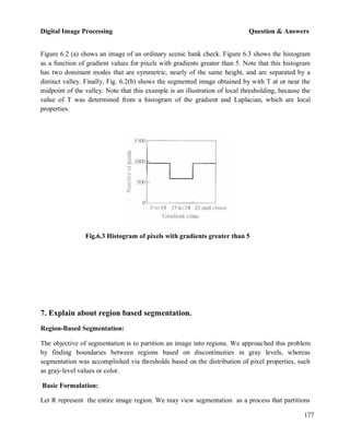
The first order of business is to determine the initial seed points. In this application, it is known
that pixels of defective welds tend to have the maximum allowable digital value B55 in this
case). Based on this information, we selected as starting points all pixels having values of 255.
The points thus extracted from the original image are shown in Fig. 10.40(b). Note that many of
the points are clustered into seed regions.
The next step is to choose criteria for region growing. In this particular
example we chose two criteria for a pixel to be annexed to a region: (1) The absolute gray-level
difference between any pixel and the seed had to be less than 65. This number is based on the
histogram shown in Fig. 7.2 and represents the difference between 255 and the location of the
first major valley to the left, which is representative of the highest gray level value in the dark
weld region. (2) To be included in one of the regions, the pixel had to be 8-connected to at least
one pixel in that region.
If a pixel was found to be connected to more than one region, the
regions were merged. Figure 7.1 (c) shows the regions that resulted by starting with the seeds in
Fig. 7.2 (b) and utilizing the criteria defined in the previous paragraph. Superimposing the
boundaries of these regions on the original image [Fig. 7.1(d)] reveals that the region-growing
procedure did indeed segment the defective welds with an acceptable degree of accuracy. It is of
interest to note that it was not necessary to specify any stopping rules in this case because the
criteria for region growing were sufficient to isolate the features of interest.
Fig.7.2 Histogram of Fig. 7.1 (a)](https://image.slidesharecdn.com/fzdjhosfqac3vchhf8as-dip-lecture-notes-230123055619-195b3297/85/DIP-LECTURE_NOTES-pdf-181-320.jpg)


![Digital Image Processing
187
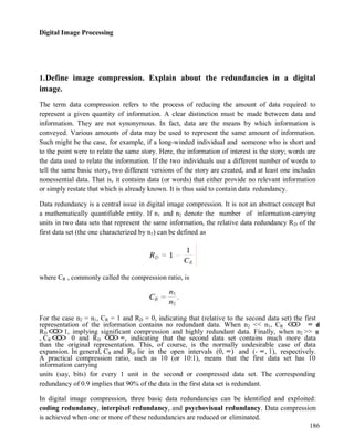
Coding Redundancy:
In this, we utilize formulation to show how the gray-level histogram of an image also can
provide a great deal of insight into the construction of codes to reduce the amount of data used to
represent it.
Let us assume, once again, that a discrete random variable rk in the interval [0, 1] represents the
gray levels of an image and that each rk occurs with probability pr (rk).
where L is the number of gray levels, nk is the number of times that the kth gray level appears in
the image, and n is the total number of pixels in the image. If the number of bits used to represent
each value of rk is l (rk), then the average number of bits required to represent each pixel is
That is, the average length of the code words assigned to the various gray-level values is found
by summing the product of the number of bits used to represent each gray level and the
probability that the gray level occurs. Thus the total number of bits required to code an M X N
image is MNLavg.
Interpixel Redundancy:
Consider the images shown in Figs. 1.1(a) and (b). As Figs. 1.1(c) and (d) show, these images
have virtually identical histograms. Note also that both histograms are trimodal, indicating the
presence of three dominant ranges of gray-level values. Because the gray levels in these images
are not equally probable, variable-length coding can be used to reduce the coding redundancy
that would result from a straight or natural binary encoding of their pixels. The coding process,
however, would not alter the level of correlation between the pixels within the images. In other
words, the codes used to represent the gray levels of each image have nothing to do with the
correlation between pixels. These correlations result from the structural or geometric
relationships between the objects in the image.](https://image.slidesharecdn.com/fzdjhosfqac3vchhf8as-dip-lecture-notes-230123055619-195b3297/85/DIP-LECTURE_NOTES-pdf-187-320.jpg)


![Digital Image Processing
194
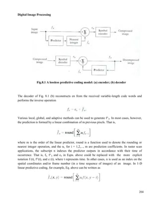
Fig. 3.2(a). In the predictive compression systems, for instance, the mapper and quantizer are
often represented by a single block, which simultaneously performs both operations.
The source decoder shown in Fig. 3.2(b) contains only two components: a symbol
decoder and an inverse mapper. These blocks perform, in reverse order, the inverse operations of
the source encoder's symbol encoder and mapper blocks. Because quantization results in
irreversible information loss, an inverse quantizer block is not included in the general source
decoder model shown in Fig. 3.2(b).
The Channel Encoder and Decoder:
The channel encoder and decoder play an important role in the overall encoding-decoding
process when the channel of Fig. 3.1 is noisy or prone to error. They are designed to reduce the
impact of channel noise by inserting a controlled form of redundancy into the source encoded
data. As the output of the source encoder contains little redundancy, it would be highly sensitive
to transmission noise without the addition of this "controlled redundancy." One of the most
useful channel encoding techniques was devised by R. W. Hamming (Hamming [1950]). It is
based on appending enough bits to the data being encoded to ensure that some minimum number
of bits must change between valid code words. Hamming showed, for example, that if 3 bits of
redundancy are added to a 4-bit word, so that the distance between any two valid code words is
3, all single-bit errors can be detected and corrected. (By appending additional bits of
redundancy, multiple-bit errors can be detected and corrected.) The 7-bit Hamming (7, 4) code
word h1, h2, h3…., h6, h7 associated with a 4-bit binary number b3b2b1b0 is
where Ⓧ denotes the exclusive OR operation. Note that bits h1, h2, and h4 are even- parity bits for
the bit fields b3 b2 b0, b3b1b0, and b2b1b0, respectively. (Recall that a string of binary bits has
even parity if the number of bits with a value of 1 is even.) To decode a Hamming encoded
result, the channel decoder must check the encoded value for odd parity over the bit fields in
which even parity was previously established. A single-bit error is indicated by a nonzero parity
word c4c2c1, where](https://image.slidesharecdn.com/fzdjhosfqac3vchhf8as-dip-lecture-notes-230123055619-195b3297/85/DIP-LECTURE_NOTES-pdf-194-320.jpg)
![Digital Image Processing
195
If a nonzero value is found, the decoder simply complements the code word bit position
indicated by the parity word. The decoded binary value is then extracted from the corrected code
word as h3h5h6h7.
4. Explain a method of generating variable length codes with an example.
Variable-Length Coding:
The simplest approach to error-free image compression is to reduce only coding redundancy.
Coding redundancy normally is present in any natural binary encoding of the gray levels in an
image. It can be eliminated by coding the gray levels. To do so requires construction of a variable-
length code that assigns the shortest possible code words to the most probable gray levels. Here,
we examine several optimal and near optimal techniques for constructing such a code. These
techniques are formulated in the language of information theory. In practice, the source symbols
may be either the gray levels of an image or the output of a gray-level mapping operation (pixel
differences, run lengths, and so on).
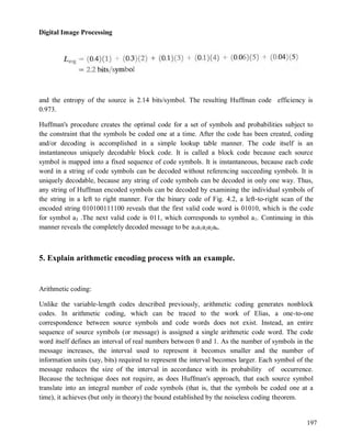
Huffman coding:
The most popular technique for removing coding redundancy is due to Huffman (Huffman
[1952]). When coding the symbols of an information source individually, Huffman coding yields
the smallest possible number of code symbols per source symbol. In terms of the noiseless
coding theorem, the resulting code is optimal for a fixed value of n, subject to the constraint that
the source symbols be coded one at a time.
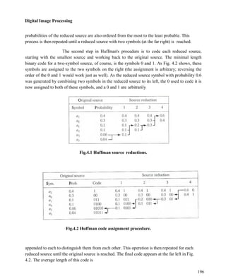
The first step in Huffman's approach is to create a series of source reductions by ordering the
probabilities of the symbols under consideration and combining the lowest probability symbols
into a single symbol that replaces them in the next source reduction. Figure 4.1 illustrates this
process for binary coding (K-ary Huffman codes can also be constructed). At the far left, a
hypothetical set of source symbols and their probabilities are ordered from top to bottom in terms
of decreasing probability values. To form the first source reduction, the bottom two probabilities,
0.06 and 0.04, are combined to form a "compound symbol" with probability 0.1. This compound
symbol and its associated probability are placed in the first source reduction column so that the](https://image.slidesharecdn.com/fzdjhosfqac3vchhf8as-dip-lecture-notes-230123055619-195b3297/85/DIP-LECTURE_NOTES-pdf-195-320.jpg)
![Digital Image Processing
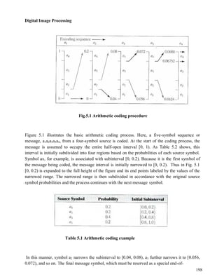
199
message indicator, narrows the range to [0.06752, 0.0688). Of course, any number within this
subinterval—for example, 0.068—can be used to represent the message.
In the arithmetically coded message of Fig. 5.1, three decimal digits are used
to represent the five-symbol message. This translates into 3/5 or 0.6 decimal digits per source
symbol and compares favorably with the entropy of the source, which is 0.58 decimal digits or 10-
ary units/symbol. As the length of the sequence being coded increases, the resulting arithmetic
code approaches the bound established by the noiseless coding theorem.
In practice, two factors cause coding performance to fall short of the bound: (1)
the addition of the end-of-message indicator that is needed to separate one message from an-
other; and (2) the use of finite precision arithmetic. Practical implementations of arithmetic
coding address the latter problem by introducing a scaling strategy and a rounding strategy
(Langdon and Rissanen [1981]). The scaling strategy renormalizes each subinterval to the [0, 1)
range before subdividing it in accordance with the symbol probabilities. The rounding strategy
guarantees that the truncations associated with finite precision arithmetic do not prevent the
coding subintervals from being represented accurately.
6. Explain LZW coding with an example.
LZW Coding:
The technique, called Lempel-Ziv-Welch (LZW) coding, assigns fixed-length code words to
variable length sequences of source symbols but requires no a priori knowledge of the
probability of occurrence of the symbols to be encoded. LZW compression has been integrated
into a variety of mainstream imaging file formats, including the graphic interchange format
(GIF), tagged image file format (TIFF), and the portable document format (PDF).
LZW coding is conceptually very simple (Welch [1984]). At the onset of the
coding process, a codebook or "dictionary" containing the source symbols to be coded is
constructed. For 8-bit monochrome images, the first 256 words of the dictionary are assigned to
the gray values 0, 1, 2..., and 255. As the encoder sequentially examines the image's pixels, gray-
level sequences that are not in the dictionary are placed in algorithmically determined (e.g., the
next unused) locations. If the first two pixels of the image are white, for instance, sequence ―255-
255‖ might be assigned to location 256, the address following the locations reserved for gray
levels 0 through 255. The next time that two consecutive white pixels are encountered, code
word 256, the address of the location containing sequence 255-255, is used to represent them. If
a 9-bit, 512-word dictionary is employed in the coding process, the original (8 + 8) bits that were](https://image.slidesharecdn.com/fzdjhosfqac3vchhf8as-dip-lecture-notes-230123055619-195b3297/85/DIP-LECTURE_NOTES-pdf-199-320.jpg)