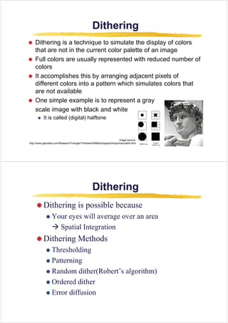
This document discusses various digital image processing techniques including dithering, warping, morphing, and view morphing. Specifically, it describes:
- Dithering techniques like thresholding, ordered dithering, and error diffusion to simulate colors not in the palette.
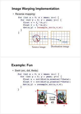
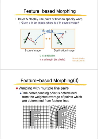
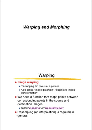
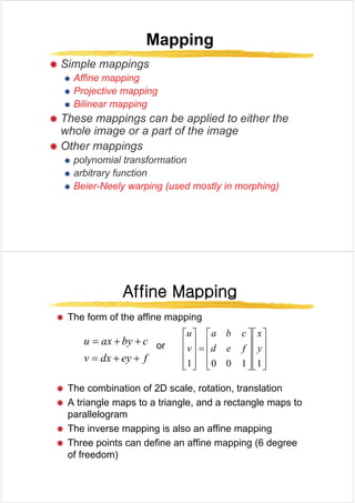
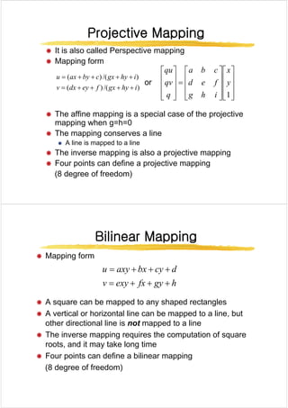
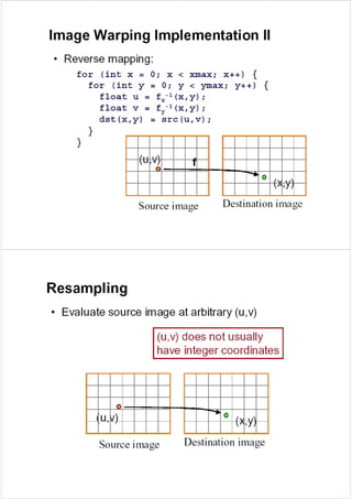
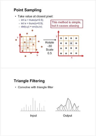
- Image warping methods like affine, projective, and bilinear mappings to rearrange pixel positions.
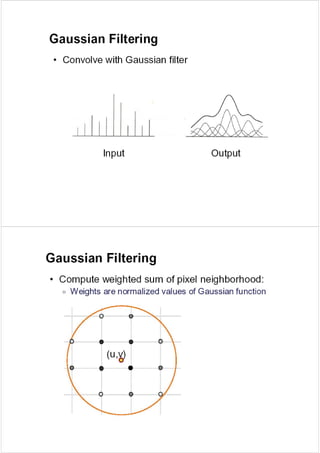
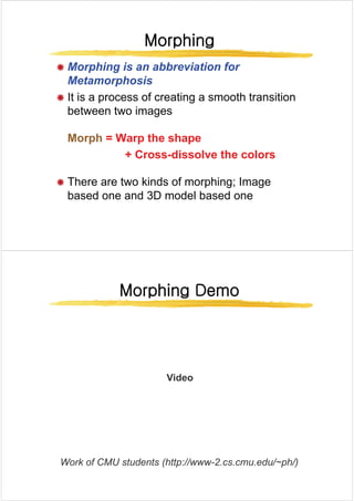
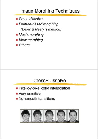
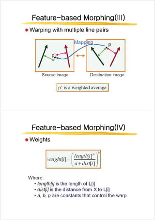
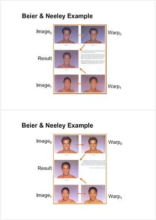
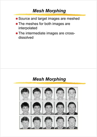
- Morphing as a process to create a smooth transition between two images using warping, color interpolation, and cross-dissolving.
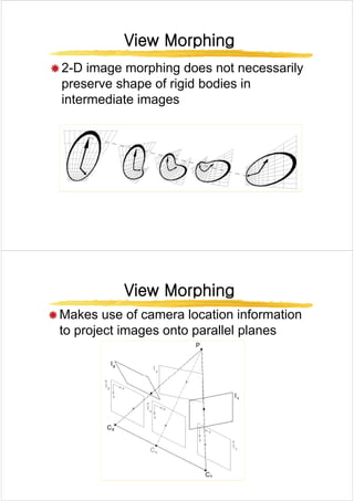
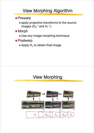
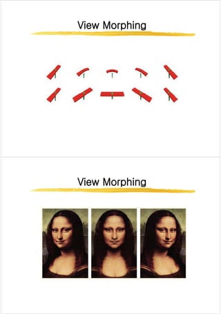
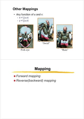
- View morphing which uses camera position to project images and preserve rigid body shapes during morphing.
The document discusses different techniques for image interpolation, which is the process of estimating unknown pixel values between known sample points in an image. It describes several 1D and 2D interpolation methods like nearest neighbor, bilinear, and bicubic interpolation. These methods are used in applications such as resolution enhancement through digital zooming, error concealment via image inpainting, and geometric transformations of images. Bicubic interpolation generally provides the smoothest results with fewest artifacts compared to other methods.
This document presents a novel algorithm that combines signature method and linear filtering techniques to detect convex polygons, specifically finder and alignment patterns, in slanted or distorted QR code images. The algorithm scans the image contour to generate a signature function, then applies linear filtering to extract high frequency components and identify vertices. It can locate multiple anchor patterns in one scan, arrange them to straighten the image. Only requiring a single scan, it is computationally efficient and suitable for real-time applications like QR code decoding.
This document discusses various techniques for enhancing images in the spatial domain, which involves direct manipulation of pixel values. It describes point processing techniques like gray-level transformations that map input pixel values to output values using functions like negative, logarithm, power-law, and piecewise linear. Histogram processing techniques are also covered, including histogram equalization, which spreads out the most frequent intensity values in an image. The document provides examples to illustrate the effect of these different enhancement methods.
This document discusses image enhancement techniques in the spatial domain. It defines spatial domain enhancement as the direct manipulation of pixel values. Some key techniques discussed include contrast stretching to improve low contrast, histogram equalization to improve contrast, sharpening filters to enhance edges using derivatives, and smoothing filters for noise reduction. The document provides examples and definitions of various spatial filters and their effects.
study Diffusion Curves: A Vector Representation for Smooth-Shaded ImagesChiamin Hsu
This document introduces diffusion curves, a new vector-based image representation. Diffusion curves represent smooth shaded images using curves that diffuse color on both sides. This allows for more complex gradients than previous methods. The document outlines how diffusion curves are created either manually, assisted via color sampling, or automatically from bitmaps. It also describes how diffusion curves are rendered by rasterizing color sources along curves, computing a gradient field, diffusing color, and reblurring. This new representation offers benefits over gradient meshes while being compact and enabling artistic control.
This document discusses various techniques for image enhancement, including point operations, mask operations, transform operations, and coloring operations. It provides details on techniques such as contrast stretching, histogram equalization, and histogram specification. Histogram equalization aims to produce an output image with a uniform histogram, while histogram specification allows specifying a desired output histogram. Both techniques involve transforming the input image using the cumulative distribution function of the input pixel values.
At the end of this lesson, you should be able to;
describe spatial resolution
describe intensity resolution
identify the effect of aliasing
describe image interpolation
describe relationships among the pixels
Image enhancement techniques aim to improve the visual quality of digital images for specific applications. The main goals are to process images to be more suitable without adding extra information. Enhancement is done in the spatial domain by directly manipulating pixel values, or in the frequency domain by modifying the image's Fourier transform. Common spatial techniques include point processing (intensity transformations) and neighborhood processing (smoothing filters). Intensity transformations like contrast stretching increase an image's dynamic range, while smoothing filters reduce noise through averaging or weighted averaging. Frequency domain techniques exploit aspects hidden in the spatial domain. Laplacian filtering and gradient operations like Roberts' method are also used for image sharpening by highlighting edges.
This document discusses single-view modeling using projective geometry. It begins with an overview of projective geometry concepts like homogeneous coordinates, duality of points and lines, and perspective projection. It then covers applications like computing vanishing points and lines from images to model the 3D scene layout. Methods for measuring object heights using cross-ratios and known reference heights are also presented. The document concludes with a discussion of related techniques like camera calibration and single-image depth prediction.
This document discusses image enhancement techniques in the spatial domain. It begins by introducing intensity transformations and spatial filtering as the two principal categories of spatial domain processing. It then describes the basics of intensity transformations, including how they directly manipulate pixel values in an image. The document focuses on different types of basic intensity transformation functions such as image negation, log transformations, power law transformations, and piecewise linear transformations. It provides examples of how these transformations can be used to enhance images. Finally, it discusses histogram processing and how the histogram of an image provides information about the distribution of pixel intensities.
This document provides an overview of key concepts in digital image fundamentals. It discusses the human visual system and image formation in the eye. It also covers image acquisition, sampling, quantization, and representation. Additionally, it defines concepts like spatial and intensity resolution and describes basic image processing operations and transforms. The goal is to introduce fundamental digital image processing concepts.
The document discusses various image enhancement techniques in the spatial domain. It describes how spatial domain techniques directly manipulate pixel values in an image. Basic approaches include gray level transformations, point processing, and histogram equalization. Gray level transformations map input pixel values to output values using functions like negation, logarithms, and power laws. Point processing methods apply operators locally within a neighborhood, such as contrast stretching. Histogram equalization spreads out the histogram of an image to increase contrast.
Here in the ppt a detailed description of Image Enhancement Techniques is given which includes topics like Basic Gray level Transformations,Histogram Processing.
Enhancement using Arithmetic/Logic Operations.
image averaging and image averaging methods.
Piecewise-Linear Transformation Functions
This document discusses pixel relationships and neighborhood concepts in digital images. It defines a pixel and pixel connectivity. There are different types of pixel neighborhoods, including 4-neighbor, 8-neighbor, and diagonal neighbors. Connected components are sets of pixels that are connected based on pixel adjacency. Algorithms can label connected components and identify distinct image regions. Various distance measures quantify how close pixels are, such as Euclidean, Manhattan, and chessboard distances. Arithmetic and logical operators can combine pixel values from different images. Neighborhood operations apply functions to pixels based on their values and those of nearby pixels.
The document provides an overview of key concepts in image processing, including definitions of digital images, image formats, data types, processing operations, and mathematical foundations. It defines what an image and digital image are, explains color models and image resolution. It also covers common image file formats, data types, the scope of image processing including low, mid, and high-level operations. Additionally, it introduces basic terms in image topology and the mathematical concepts of image formation, properties of the point spread function, and linear shift-invariance and convolution.
Interactive Stereoscopic Rendering for Non-Planar Projections (GRAPP 2009)Matthias Trapp
This document discusses approaches for interactive stereo rendering of 3D environments with non-planar projections. It compares a geometry-based approach (GBA) and an image-based approach (IBA) in terms of implementation complexity, memory footprint, rendering performance, and image quality. The GBA outperforms the IBA in rendering and image quality but is more complex and has a larger memory footprint for high field-of-view projections. The IBA is easier to implement but has artifacts from cubemap sampling. Future work is proposed to improve the IBA's performance and image quality.
The document discusses several basic image processing operations in OpenCV including flipping, rotating, resizing, cropping, and extracting color channels. Flipping uses cv2.flip() and takes an image and flip direction. Rotation uses cv2.rotate() and takes an image and rotation angle. Resizing uses cv2.resize() and takes an image and new dimensions. Cropping extracts a region of an image by specifying dimensions. Color channel extraction uses cv2.split() and cv2.merge() with NumPy arrays of zeros to isolate individual color channels in BGR order.
This document describes a project to develop a pedestrian detection system and lane detection and warning system for medium-class cars. It is created by group members Sanket R. Borhade, Manthan N. Shah, and Pravin D. Jadhav.
The document outlines the need for such systems to reduce traffic accidents and pedestrian fatalities. It then describes the existing technologies for lane detection and pedestrian detection systems. The document provides detailed explanations of the methods and algorithms used in their proposed lane detection system, including Hough transforms and lane identification. It also explains the use of Haar features, AdaBoost, and edgelet features in their proposed pedestrian detection system. Finally, it presents results from testing their systems and
This document provides an overview of key concepts in image processing, including:
- Digital image representation as a 2D array of integer pixel values
- Image acquisition through illumination of a scene and absorption of reflected energy by image sensors
- Sampling and quantization to convert a continuous image into discrete digital values
- Spatial and intensity resolution which determine image quality
- Common image file formats and operations like filtering, arithmetic/logical operations, and basic geometric transformations including translation, rotation, scaling and shearing.
This document discusses image features and their representation. It defines image features as a reduced representation of input image data. The main types of features discussed are pixel-level, local, and global features. Local features include edge detection, corner detection, and color features. Color features can be represented using histograms that count the number of pixels for each color value. The document also discusses different techniques for representing detected edges, including simple representation, chain codes, slope representation and signatures. Histograms are described as a common method for color feature representation.
The document provides information about computer graphics concepts including:
1. Summarizing questions and answers about 3D triangles, rotation matrices, vector operations, splines, and computer graphics techniques like environment mapping and anti-aliasing.
2. Explaining modifications made to the active edge list algorithm to enable scan conversion of different triangle types like smoothly shaded, textured, and environment mapped triangles.
3. Deriving the 4x4 projection matrix that maps a 3D object point to its shadow point on a plane, to create planar shadows.
beginning with a tree T containing a single vertex
repeatedly adding the least cost edge between T and the rest of the graph
terminating when T spans all vertices
- The document discusses graphs and graph algorithms including definitions of graph terminology, representations of graphs, graph traversal algorithms like depth-first search and breadth-first search, and algorithms for finding minimum spanning trees like Kruskal's algorithm and Prim's algorithm.
- It provides detailed descriptions and pseudocode for graph traversal algorithms, algorithms to find connected components and articulation points, and minimum cost spanning tree algorithms.
- The document is intended as a curriculum for teaching graph algorithms and data structures.
To create a digital image from a continuous sensed image, sampling and quantization must occur. Sampling involves digitizing the coordinate values to reduce the image to a series of amplitude values over time. Quantization digitizes the amplitude values by rounding them to the nearest value in a defined set of possible values. Together, sampling and quantization convert a continuous image into a digital form by discretizing both the coordinates and amplitudes.
Similar to Digital_Image_Processing_Digital_Image_Processing_Dithering_.pdf (20)
Open Channel Flow: fluid flow with a free surfaceIndrajeet sahu
Open Channel Flow: This topic focuses on fluid flow with a free surface, such as in rivers, canals, and drainage ditches. Key concepts include the classification of flow types (steady vs. unsteady, uniform vs. non-uniform), hydraulic radius, flow resistance, Manning's equation, critical flow conditions, and energy and momentum principles. It also covers flow measurement techniques, gradually varied flow analysis, and the design of open channels. Understanding these principles is vital for effective water resource management and engineering applications.
Software Engineering and Project Management - Introduction, Modeling Concepts...Prakhyath Rai
Introduction, Modeling Concepts and Class Modeling: What is Object orientation? What is OO development? OO Themes; Evidence for usefulness of OO development; OO modeling history. Modeling
as Design technique: Modeling, abstraction, The Three models. Class Modeling: Object and Class Concept, Link and associations concepts, Generalization and Inheritance, A sample class model, Navigation of class models, and UML diagrams
Building the Analysis Models: Requirement Analysis, Analysis Model Approaches, Data modeling Concepts, Object Oriented Analysis, Scenario-Based Modeling, Flow-Oriented Modeling, class Based Modeling, Creating a Behavioral Model.
Home security is of paramount importance in today's world, where we rely more on technology, home
security is crucial. Using technology to make homes safer and easier to control from anywhere is
important. Home security is important for the occupant’s safety. In this paper, we came up with a low cost,
AI based model home security system. The system has a user-friendly interface, allowing users to start
model training and face detection with simple keyboard commands. Our goal is to introduce an innovative
home security system using facial recognition technology. Unlike traditional systems, this system trains
and saves images of friends and family members. The system scans this folder to recognize familiar faces
and provides real-time monitoring. If an unfamiliar face is detected, it promptly sends an email alert,
ensuring a proactive response to potential security threats.
DEEP LEARNING FOR SMART GRID INTRUSION DETECTION: A HYBRID CNN-LSTM-BASED MODELijaia
As digital technology becomes more deeply embedded in power systems, protecting the communication
networks of Smart Grids (SG) has emerged as a critical concern. Distributed Network Protocol 3 (DNP3)
represents a multi-tiered application layer protocol extensively utilized in Supervisory Control and Data
Acquisition (SCADA)-based smart grids to facilitate real-time data gathering and control functionalities.
Robust Intrusion Detection Systems (IDS) are necessary for early threat detection and mitigation because
of the interconnection of these networks, which makes them vulnerable to a variety of cyberattacks. To
solve this issue, this paper develops a hybrid Deep Learning (DL) model specifically designed for intrusion
detection in smart grids. The proposed approach is a combination of the Convolutional Neural Network
(CNN) and the Long-Short-Term Memory algorithms (LSTM). We employed a recent intrusion detection
dataset (DNP3), which focuses on unauthorized commands and Denial of Service (DoS) cyberattacks, to
train and test our model. The results of our experiments show that our CNN-LSTM method is much better
at finding smart grid intrusions than other deep learning algorithms used for classification. In addition,
our proposed approach improves accuracy, precision, recall, and F1 score, achieving a high detection
accuracy rate of 99.50%.
Applications of artificial Intelligence in Mechanical Engineering.pdfAtif Razi
Historically, mechanical engineering has relied heavily on human expertise and empirical methods to solve complex problems. With the introduction of computer-aided design (CAD) and finite element analysis (FEA), the field took its first steps towards digitization. These tools allowed engineers to simulate and analyze mechanical systems with greater accuracy and efficiency. However, the sheer volume of data generated by modern engineering systems and the increasing complexity of these systems have necessitated more advanced analytical tools, paving the way for AI.
AI offers the capability to process vast amounts of data, identify patterns, and make predictions with a level of speed and accuracy unattainable by traditional methods. This has profound implications for mechanical engineering, enabling more efficient design processes, predictive maintenance strategies, and optimized manufacturing operations. AI-driven tools can learn from historical data, adapt to new information, and continuously improve their performance, making them invaluable in tackling the multifaceted challenges of modern mechanical engineering.
Generative AI Use cases applications solutions and implementation.pdfmahaffeycheryld
Generative AI solutions encompass a range of capabilities from content creation to complex problem-solving across industries. Implementing generative AI involves identifying specific business needs, developing tailored AI models using techniques like GANs and VAEs, and integrating these models into existing workflows. Data quality and continuous model refinement are crucial for effective implementation. Businesses must also consider ethical implications and ensure transparency in AI decision-making. Generative AI's implementation aims to enhance efficiency, creativity, and innovation by leveraging autonomous generation and sophisticated learning algorithms to meet diverse business challenges.
https://www.leewayhertz.com/generative-ai-use-cases-and-applications/
1. Digital Image Processing
Digital Image Processing
(UST 2007 Fall
(UST 2007 Fall)
)
(UST 2007 Fall
(UST 2007 Fall)
)
Sang Chul Ahn
asc@imrc.kist.re.kr
asc@imrc.kist.re.kr
Dithering
Dithering
2. Dithering
Dithering
Dithering
Dithering
Æ Dithering is a technique to simulate the display of colors
g q p y
that are not in the current color palette of an image
Æ Full colors are usually represented with reduced number of
colors
Æ It accomplishes this by arranging adjacent pixels of
different colors into a pattern which simulates colors that
are not available
Æ O i l l i t t
Æ One simple example is to represent a gray
scale image with black and white
It is called (digital) halftone
Æ It is called (digital) halftone
image source:
http://www.geocities.com/ResearchTriangle/Thinktank/5996/techpaps/introip/manual04.html
Dithering
Dithering
Dithering
Dithering
Æ Dithering is possible because
Æ Your eyes will average over an area
Æ S i l i
Æ Spatial Integration
Æ Dithering Methods
g
Æ Thresholding
Æ Patterning
Æ Patterning
Æ Random dither(Robert’s algorithm)
Æ Ordered dither
Æ Error diffusion
3. Thresholding
Thresholding
Thresholding
Thresholding
Æ A simple fixed threshold can be used but
Æ A simple fixed threshold can be used, but
average intensity for a threshold can give a
good(?) result Æ Average thresholding
image source: http://en.wikipedia.org/wiki/Dither
Patterning
Patterning
Patterning
Patterning
Æ Patterning is used when the spatial resolution
of an output is greater than that of a source
image
image
Æ It generates an image that is of higher spatial
resolution than the source image
Æ Compute the intensity of each sub-block(or
pixel) and index a pattern
Æ Pattern should grow as the intensity gets
brighter
Æ The 1’s pixels in the previous level pattern should
b d i h l l
be preserved in the next level
5. Random Dithering
Random Dithering
Random Dithering
Random Dithering
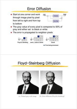
Æ Add a random amount to each pixel before thresholding
p g
Æ Typically add uniformly random amount from [-a,a]
Æ Pure addition of noise to the image
Æ Not good for black and white, but OK for more colors
Æ Add a small random color to each pixel before finding the
l t l i th t bl
closest color in the table
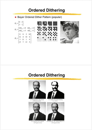
Ordered Dithering
Ordered Dithering
Ordered Dithering
Ordered Dithering
Æ Break the image into small blocks
Æ Define a threshold matrix
Æ Use a different threshold for each pixel of the block
Æ Compare each pixel to its own threshold
Æ The thresholds can be clustered, which looks like a
(di it l) h lft i
newspaper: (digital) halftoning
Æ The thresholds can be “random” which looks better
7. Error Diffusion
Error Diffusion
Error Diffusion
Error Diffusion
Æ Start at one corner and work
through image pixel by pixel
from left to right and from top
to bottom
Æ The gray value of every pixel is compared to 50% of
gray and either set to black or white
Æ The error is propagated to neighbor pixels
p p g g p
Floyd
Floyd-
-Steinberg Diffusion
Steinberg Diffusion
Floyd
Floyd Steinberg Diffusion
Steinberg Diffusion
9. Warping and Morphing
Warping and Morphing
Warping
Warping
Warping
Warping
Æ
Æ Image warping
Image warping
Æ
Æ Image warping
Image warping
Æ rearranging the pixels of a picture
Æ Also called “image distortion” “geometric image
Æ Also called image distortion , geometric image
transformation”
Æ We need a function that maps points between
corresponding points in the source and
destination images
destination images
Æ called “mapping” or “transformation”
Æ Resampling (or interpolation) is required in
general
10. Mapping
Mapping
Mapping
Mapping
Æ Simple mappings
Æ Affine mapping
Æ Projective mapping
Æ Bilinear mapping
Æ These mappings can be applied to either the
whole image or a part of the image
Æ Other mappings
Æ polynomial transformation
Æ arbitrary function
Æ Beier-Neely warping (used mostly in morphing)
Affine Mapping
Affine Mapping
Affine Mapping
Affine Mapping
Æ The form of the affine mapping
pp g
or
c
by
ax
u +
+
=
⎥
⎥
⎤
⎢
⎢
⎡
⎥
⎥
⎤
⎢
⎢
⎡
=
⎥
⎥
⎤
⎢
⎢
⎡
y
x
f
e
d
c
b
a
v
u
f
ey
dx
v +
+
= ⎥
⎥
⎦
⎢
⎢
⎣
⎥
⎥
⎦
⎢
⎢
⎣
=
⎥
⎥
⎦
⎢
⎢
⎣ 1
1
0
0
1
y
f
e
d
v
Æ The combination of 2D scale, rotation, translation
Æ A triangle maps to a triangle, and a rectangle maps to
parallelogram
Æ The inverse mapping is also an affine mapping
pp g pp g
Æ Three points can define an affine mapping (6 degree
of freedom)
11. Projective Mapping
Projective Mapping
Projective Mapping
Projective Mapping
Æ It is also called Perspective mapping
Æ Mapping form
)
/(
)
( i
hy
gx
c
by
ax
u +
+
+
+
= ⎥
⎤
⎢
⎡
⎥
⎤
⎢
⎡
⎥
⎤
⎢
⎡ x
f
d
c
b
a
qu
or
)
/(
)
(
)
(
)
(
i
hy
gx
f
ey
dx
v
y
g
y
+
+
+
+
=
⎥
⎥
⎥
⎦
⎢
⎢
⎢
⎣
⎥
⎥
⎥
⎦
⎢
⎢
⎢
⎣
=
⎥
⎥
⎥
⎦
⎢
⎢
⎢
⎣ 1
y
i
h
g
f
e
d
q
qv
Æ The affine mapping is a special case of the projective
mapping when g=h=0
mapping when g h 0
Æ The mapping conserves a line
Æ A line is mapped to a line
Æ The inverse mapping is also a projective mapping
Æ Four points can define a projective mapping
(8 degree of freedom)
Bilinear Mapping
Bilinear Mapping
Bilinear Mapping
Bilinear Mapping
Æ Mapping form
h
gy
fx
exy
v
d
cy
bx
axy
u
+
+
+
=
+
+
+
=
Æ A square can be mapped to any shaped rectangles
h
gy
fx
exy
v +
+
+
=
q pp y p g
Æ A vertical or horizontal line can be mapped to a line, but
other directional line is not mapped to a line
Æ The inverse mapping requires the computation of square
roots, and it may take long time
Æ Four points can define a bilinear mapping
(8 degree of freedom)
17. Bilinear Interpolation
Bilinear Interpolation
Æ A B C D are intensity s )
1
( s
A B
E
Æ A,B,C,D are intensity
values t
s )
1
( s
−
A B
E
sB
A
s
E +
−
= )
1
( )
1
( t
G
sD
C
s
F
sB
A
s
E
+
−
=
+
)
1
(
)
1
( )
1
( t
−
C D
tF
E
t
G +
−
= )
1
(
[ ] [ ]
sD
C
s
t
sB
A
s
t +
−
+
+
−
−
= )
1
(
)
1
(
)
1
(
C D
F
[ ] [ ]
tsD
C
s
t
sB
t
A
s
t
sD
C
s
t
sB
A
s
t
+
−
+
−
+
−
−
=
+
+
+
=
)
1
(
)
1
(
)
1
)(
1
(
)
1
(
)
1
(
)
1
(
18.
19.
20. Morphing
Morphing
Morphing
Morphing
Æ Morphing is an abbreviation for
Metamorphosis
Æ It is a process of creating a smooth transition
between two images
Morph
Morph = Warp the shape
= Warp the shape
+ Cross
+ Cross dissolve the colors
dissolve the colors
+ Cross
+ Cross-
-dissolve the colors
dissolve the colors
Æ There are two kinds of morphing; Image
based one and 3D model based one
Morphing Demo
Morphing Demo
Morphing Demo
Morphing Demo
Vid
Video
W k f CMU t d t (htt // 2 d / h/)
Work of CMU students (http://www-2.cs.cmu.edu/~ph/)
22. Feature
Feature-
-based Morphing
based Morphing
Feature
Feature based Morphing
based Morphing
Feature
Feature-
-based Morphing(II)
based Morphing(II)
Feature
Feature based Morphing(II)
based Morphing(II)
Æ Warping with multiple line pairs
Æ The corresponding point is determined
from the weighted average of points which
are determined from feature lines
23. Feature
Feature-
-based Morphing(III)
based Morphing(III)
Feature
Feature based Morphing(III)
based Morphing(III)
Æ Warping with multiple line pairs
Feature
Feature-
-based Morphing(IV
based Morphing(IV)
)
Feature
Feature based Morphing(IV
based Morphing(IV)
)
Æ Weights
Æ Weights
24.
25. Mesh Morphing
Mesh Morphing
Mesh Morphing
Mesh Morphing
Æ Source and target images are meshed
Æ The meshes for both images are
i t l t d
interpolated
Æ The intermediate images are cross-
Æ The intermediate images are cross
dissolved
Mesh Morphing
Mesh Morphing
Mesh Morphing
Mesh Morphing
26. View Morphing
View Morphing
View Morphing
View Morphing
Æ 2-D image morphing does not necessarily
Æ 2 D image morphing does not necessarily
preserve shape of rigid bodies in
intermediate images
intermediate images
View Morphing
View Morphing
View Morphing
View Morphing
Æ Makes use of camera location information
to project images onto parallel planes
27. View Morphing Algorithm
View Morphing Algorithm
Æ Prewarp
Æ Prewarp
Æ apply projective transforms to the source
images (H -1 and H -1)
images (H0
-1 and H1
-1)
Æ Morph
Æ Use any image morphing technique
Æ Postwarp
Æ Postwarp
Æ Apply Hs to obtain final image
View Morphing
View Morphing
View Morphing
View Morphing