#1 If this PowerPoint presentation contains mathematical equations, you may need to check that your computer has the following installed:
1) MathType Plugin
2) Math Player (free versions available)
3) NVDA Reader (free versions available)
#19 Long Description:
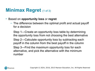
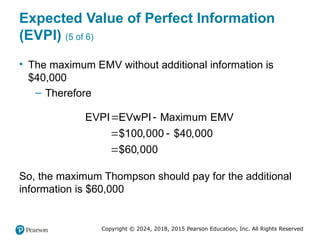
E M V, left parenthesis, alternative i, right parenthesis, equals, left parenthesis, payoff of first state of nature, right parenthesis, times, left parenthesis, probability of first state of nature, right parenthesis, plus, left parenthesis, payoff of second state of nature, right parenthesis, times, left parenthesis, probability of second state of nature, right parenthesis, plus, ellipsis, plus, left parenthesis, payoff of last state of nature, right parenthesis, times, left parenthesis, probability of last state of nature, right parenthesis.
#28 Long description:
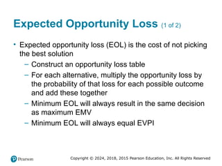
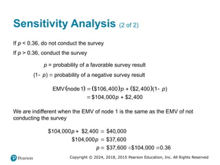
E O L, left parenthesis, large plant, right parenthesis, equals, left parenthesis, 0.50, right parenthesis, times, left parenthesis, 0 dollar, right parenthesis, plus, left parenthesis, 0.50, right parenthesis times left parenthesis, 180,000 dollars, right parenthesis, equals 90,000 dollars. E O L, left parenthesis, small plant, right parenthesis, equals, left parenthesis, 0.50, right parenthesis, times, left parenthesis, 100,000 dollars, right parenthesis, plus, left parenthesis, 0.50, right parenthesis, times, left parenthesis, 20,000 dollars, right parenthesis, equals 60,000 dollars. E O L, left parenthesis, do nothing, right parenthesis, equals, left parenthesis, 0.50, right parenthesis, times, left parenthesis, 200,000 dollars, right parenthesis, plus, left parenthesis, 0.50, right parenthesis, times, left parenthesis, 0 dollar, right parenthesis, equals 100,000 dollars.
#29 Long Description:
E M V, left parenthesis, large plant, right parenthesis, equals, 200,000 dollars P minus 180,000 dollars, right parenthesis, times, left parenthesis, 1 minus P, right parenthesis, equals 200,000 dollars P minus 180,000 dollars plus 180,000 dollars P equals 380,000 dollars P minus 180,000 dollars. E M V, left parenthesis, small plant, right parenthesis equals 100,000 dollars P minus 20,000 dollars, right parenthesis, times, left parenthesis, 1 minus P, right parenthesis, equals 100,000 dollars P minus 20,000 dollars plus 20,000 dollars P equals 120,000 dollars P minus 20,000 dollars. E M V, left parenthesis, do nothing, right parenthesis, equals 0 dollar P plus 0, times, left parenthesis, 1 minus P, right parenthesis, equals 0 dollar.
#30 Long Description:
The graph’s y axis is labeled E M V Value and is scaled in units of one hundred thousand dollars from negative two hundred thousand dollars to positive three hundred thousand dollars. The X axis, labeled Value of P, originates from the zero point on the y axis and has three data points labeled 0.167, 0.615, and 1.
The x axis represents an E M V, do nothing. There is a line that originates from the negative two hundred thousand dollar point of the y axis and ascends up and to the right, crossing the x axis right before the data point of 0.61. It ends on the far right of the x axis, parallel to the positive two hundred thousand dollar point of the y axis. It is marked as E M V, large plant.
A second line originates just under the zero point of the y axis, it ascends up and to the right, crossing the x axis exactly at the 0.167 mark. This intersection is labeled Point One. This same line continues ascending and intersects the first line at the 0.615 data mark, this intersection is labeled Point Two. It ends on the far right of the x axis, parallel to the positive one hundred thousand dollar point of the y axis. It is marked as E M V, small plant.
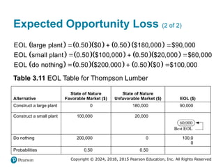
#33 Hurwicz criterion with 70% coefficient
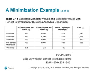
Machine A = 0.7×950+0.3×1150=1010
Machine B = 0.7×850+0.3×1350=1000
Machine C = 0.7×700+0.3×1300=880 → Choose C
Equally likely criterion
Machine A = (950+1050+1150)/3 = 1050
Machine B = (850+1100+1350)/3 = 1100
Machine C = (700+1000+1300)/3 = 1000 → Choose C
EMV criterion
Machine A = 950×0.4+1050×0.3+1150×0.3 = 1040
Machine B = 850×0.4+1100×0.3+1350×0.3 = 1075
Machine C = 700×0.4+1000×0.3+1300×0.3 = 970 → Choose C
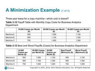
#36 Long Description:
A tip box gives instructions to enter data into table and type the row and column names. The words Thompson Lumber appear on the upper right row of the Excel screen. There are three columns of five cells each underneath Thompson Lumber.
The input in the first column, descending, is as follows,
First cell is blank
Probabilities
Large Plant
Small Plant
Do Nothing
The input in the second column, descending, is as follows,
Favorable market
0.5
200,000
100,000
Zero
The input in the third column, descending, is as follows,
Unfavorable market
0.5
Negative 180000
Negative 20000
Zero
#37 Long Description:
The pop up window is labeled Decision Table Results. There are a minus sign, square, and x on the upper right corner of the pop up.
The output is in the form of a table titled Thompson Lumber Solutions. The table contains seven columns of seven rows each.
The data in column one, descending, is as follows,
The first cell is blank
Probabilities
Large Plant
Small Plant
Do Nothing
The data in column two, descending, is as follows,
Favorable Market
0.5
200,000
100,000
Zero
The sixth cell is blank
The seventh cell is blank
The data in column three, descending, is as follows,
Unfavorable Market
0.5
Negative 180000
Negative 20000
Zero
Maximum
The seventh cell is blank
The data in column four, descending, is as follows,
E M V
The second cell is blank
10000
40000
Zero
40000
Best E V
The data in column five, descending, is as follows,
Row Min
The second cell is blank
Negative 180000
Negative 20000
Zero
Zero
Maximin
The data in column six, descending, is as follows,
Row Max
The second cell is blank
200000
100000
Zero
200000
Maximax
The data in column seven, descending, is as follows,
Hurwicz
The second cell is blank
86000
64000
Zero
860000
Best Hurwicz
Underneath the table, the following text appears, The maximum expected monetary value is 40000 given by Small Plant. The maximin is zero given by Do Nothing. The maximax is 200000 given by Large Plant.
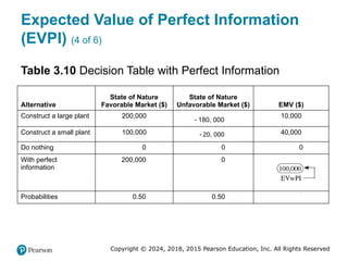
#38 Long Description:
A tip box provides guidance that To see the formulas, hold down the control key left parenthesis C t r l right parenthesis and press the grave accent key, which is usually found above the Tab key. A pop up box on the Excel chart instructs you to enter the profits in the main body of the data table. Enter probabilities in the first row if you want to compute the expected value. The screenshot is divided roughly into three vertical sections. The top section spans rows seven through twelve. The middle section spans rows fourteen through seventeen. The bottom section spans rows nineteen through twenty five.
The topmost third consists of two data tables. The first data table contains three columns, labeled Profit, Favorable Market, and Unfavorable Market. Input for the Profit column, descending, is as follows, Probability, Large plant, Small plant, and Do nothing. Input for the Favorable Market, descending, is as follows, 0.5, 200000, 100000, and zero. Input for the Unfavorable Market column, descending, is as follows, 0.5, negative 180000, negative 20000, and zero.
The second data table is adjacent to the first table, a single blank column, column D, separates the two. This second table contains three columns, labeled E M V, Minimum, and Maximum. Input for the E M V column, descending, is BLANK, 10000, 40000, and zero. Input for the Minimum column, descending, is BLANK, negative 180000, negative 20000, and zero. Input for the Maximum column, descending, is BLANK, 200000, 100000, and zero. Underneath this table is a row titled Maximum. 40000 appears under the E M V column, zero appears underneath the minimum column, and 200000 appears underneath the maximum column.
The middle third begins with the following text in row fourteen, Expected value of perfect information. Row fifteen, cell A reads Column best. Row fifteen, cell B contains the number 200000 and row fifteen, column C contains the number zero.
To the right of that is a table that spans two columns, D and E. Column D is blank, Column E contains the following numbers, descending, 100000 (labeled Expected value WITH perfect information), 40000 (labeled Best expected value), and 60000 (labeled Expected value OF perfect information.
The bottom third of the chart begins with row nineteen, which reads Regret. Underneath that word is a table that spans Columns A through F. The data in this table is as follows,
Column A, descending,
Blank cell
Probability
Large plant
Small plant
Do nothing
Column B, descending,
Favorable Market
0.5
Zero
100000
200000
Column C, descending,
Unfavorable Market
0.5
180000
20000
Zero
Column D, descending,
Blank cell
Blank cell
Blank cell
Blank cell
Blank cell
Minimum
Column E, descending,
Expected
Blank cell
90000
60000
100000
60000
Column F, descending,
Maximum
Blank cell
180000
100000
200000
100000
#39 Long Description:
This screenshot focuses in on the E M V, Minimum, Maximum table from the top third of the output screen, the Expected Value table from the middle third of the output screen, and the Expected, Maximum information from the bottom third of the output screen. The screenshot shows three columns, E, F, and G, and rows nine through twenty five.
Data in Column E, descending, are as follows,
Equals SUM PRODUCT left parenthesis B dollar sign 8
Equals SUM PRODUCT left parenthesis B dollar sign 8
Equals SUM PRODUCT left parenthesis B dollar sign 8
Equal MAX left parenthesis E 9 colon E 11
Blank cell
Blank cell
Equals SUM PRODUCT left parenthesis B dollar sign 8
Equals E 12
Equals E 15 minus E 12
Blank cell
Blank cell
Expected
Blank cell
Equals SUM PRODUCT left parenthesis B dollar sign 8
Equals SUM PRODUCT left parenthesis B dollar sign 8
Equals SUM PRODUCT left parenthesis B dollar sign 8
Equals MIN left parenthesis E 22 colon E 24
Data in Column F, descending, are as follows,
Equals MIN left parenthesis B 9 colon C 9 right parenthesis
Equals MIN left parenthesis B 10 colon C 10 right parenthesis
Equals MIN left parenthesis B 11 colon C 11 right parenthesis
Equals MAX left parenthesis F 9 colon F 11 right parenthesis
Blank cell
Blank cell
Expected value under certainty
Best expected value
Expected value of perfect information
Blank cell
Blank cell
Maximum
Blank cell
Equals MAX left parenthesis B 22 colon C 22 right parenthesis
Equals MAX left parenthesis B 23 colon C 23 right parenthesis
Equals MAX left parenthesis B 24 colon C 24 right parenthesis
Equals MIN left parenthesis F 22 colon F 24 right parenthesis
Data in Column G, descending, are as follows,
Equals MAX left parenthesis B 9 colon C 9 right parenthesis
Equals MAX left parenthesis B 10 colon C 10 right parenthesis
Equals MAX left parenthesis B 11 colon C 11 right parenthesis
Equals MAX left parenthesis G 9 colon G 11 right parenthesis
#42 Long Description:
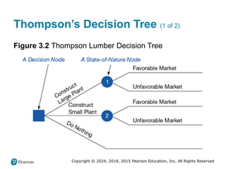
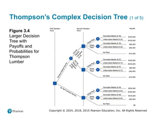
The first line is labeled construct large plant and extends to state-of-nature node 1. Two lines, labeled favorable market and unfavorable market, extend from this node. The second line from the decision node is labeled construct small plant and extends to state-of-nature node 2. Two lines, labeled favorable market and unfavorable market, extend from this node. The third line from the decision node is labeled do nothing.
#43 Long Description:
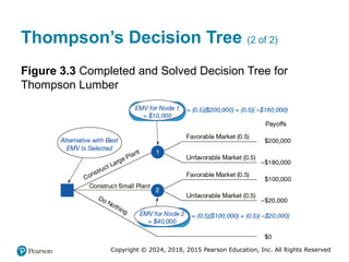
State of Nature Node 2 is labeled E M V for Node 2 equals forty thousand dollars. Formulas and payoff amounts are included on the tree. State of Nature Node 1 has the following formula next to it, The sum of 0.5 times two hundred thousand dollars added to the sum of 0.5 times negative one hundred and eighty thousand dollars. State of Nature Node 2 has the following formula next to it, The sum of 0.5 times one hundred thousand dollars added to the sum of 0.5 times negative twenty thousand dollars.
The Favorable and Unfavorable Market branches all include the number 0.5 at the end of their title, payoff amounts are listed as follows,
Construct Large Plant, Favorable Market equals two hundred thousand dollars
Construct Large Plant, Unfavorable Market equals negative one hundred and eighty thousand dollars
Construct Small Plant, Favorable Market equals one hundred thousand dollars
Construct Small Plant, Unfavorable Market equals negative twenty thousand dollars
Do Nothing equals zero
#44 Long Description:
Two additional branches come off the Conduct Market Survey branch, Survey Results Favorable left parenthesis 0.45 right parenthesis and Survey Results Negative left parenthesis 0.55 right parenthesis. There is now a vertical row of three square decision nodes marked Second Decision Point that leads to branches for plant construction options and payoff amounts.
The data on the decision tree from the Second Decision Point is as follows,
The square decision node stemming from favourable survey results branches into five additional branches,
Large Plant, State of Nature Node 2, Favorable Market left parenthesis 0.78 right parenthesis equals a payoff of one hundred and ninety thousand dollars.
Large Plant, State of Nature Node 2, Unfavorable Market left parenthesis 0.22 right parenthesis equals a payoff of negative one hundred and ninety thousand dollars.
Small Plant, State of Nature Node 3, Favorable Market left parenthesis 0.78 right parenthesis equals a payoff of ninety thousand dollars.
Small Plant, State of Nature Node 3, Unfavorable Market left parenthesis 0.22 right parenthesis equals a payoff of negative thirty thousand dollars.
No plant equals a payoff of negative ten thousand dollars.
The square decision node stemming from negative survey results branches into five additional branches,
Large Plant, State of Nature Node 4, Favorable Market left parenthesis 0.27 right parenthesis equals a payoff of one hundred and ninety thousand dollars.
Large Plant, State of Nature Node 4, Unfavorable Market left parenthesis 0.73 right parenthesis equals a payoff of negative one hundred and ninety thousand dollars.
Small Plant, State of Nature Node 5, Favorable Market left parenthesis 0.27 right parenthesis equals a payoff of ninety thousand dollars.
Small Plant, State of Nature Node 3, Unfavorable Market left parenthesis 0.73 right parenthesis equals a payoff of negative thirty thousand dollars.
No plant equals a payoff of negative ten thousand dollars.
The square decision node stemming from Do Not Conduct Survey branches into five additional branches,
Large Plant, State of Nature Node 6, Favorable Market left parenthesis 0.50 right parenthesis equals a payoff of two hundred thousand dollars.
Large Plant, State of Nature Node 6, Unfavorable Market left parenthesis 0.50 right parenthesis equals a payoff of negative one hundred and eighty thousand dollars.
Small Plant, State of Nature Node 7, Favorable Market left parenthesis 0.50 right parenthesis equals a payoff of one hundred thousand dollars.
Small Plant, State of Nature Node 7, Unfavorable Market left parenthesis 0.50 right parenthesis equals a payoff of negative twenty thousand dollars.
No plant equals a payoff of zero.
#45 Long Description:
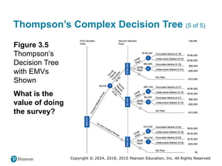
Equals E M V, left parenthesis, large plant vertical bar positive survey, right parenthesis, equals, left parenthesis, 0.78, right parenthesis, left parenthesis, 190,000 dollars, right parenthesis, plus, left parenthesis, 0.22, right parenthesis, left parenthesis, negative 190,000 dollars, right parenthesis, equals 106,400 dollars. E M V, node 3, equals E M V, left parenthesis, small plant vertical bar positive survey, right parenthesis, equals, left parenthesis, 0.78, right parenthesis, left parenthesis, 90,000 dollars, right parenthesis, plus, left parenthesis, 0.22, right parenthesis, left parenthesis, negative 30,000 dollars, right parenthesis, equals 63,600 dollars. E M V for no plant equals negative 10,000.
#46 Long Description:
Equals E M V, left parenthesis, large plant vertical bar negative survey, right parenthesis, equals, left parenthesis, 0.27, right parenthesis, left parenthesis, 190,000 dollars, right parenthesis, plus, left parenthesis, 0.73, right parenthesis, left parenthesis, negative 190,000 dollars, right parenthesis, equals negative 87,400 dollars. E M V, node 5, equals E M V, left parenthesis, small plant vertical bar negative survey, right parenthesis, equals, left parenthesis, 0.27, right parenthesis, left parenthesis, 90,000 dollars, right parenthesis, plus, left parenthesis, 0.73, right parenthesis, left parenthesis, negative 30,000 dollars, right parenthesis, equals 2,400 dollars. E M V for no plant equals negative 10,000.
#47 Long Description:
Equals E M V, left parenthesis, large plant, right parenthesis, equals, left parenthesis, 0.50, right parenthesis, left parenthesis, 200,000 dollars, right parenthesis, plus, left parenthesis, 0.50, right parenthesis, left parenthesis, negative 180,000 dollars, right parenthesis, equals 10,000 dollars. E M V, node 7, equals E M V, left parenthesis, small plant, right parenthesis, equals, left parenthesis, 0.50, right parenthesis, left parenthesis, 100,000 dollars, right parenthesis, plus, left parenthesis, 0.50, right parenthesis, left parenthesis, negative 20,000 dollars, right parenthesis, equals 40,000 dollars. E M V for no plant equals 0 dollar.
#48 Long Description:
The first decision point is at 49,200 dollars. The first decision point branches out into two as follows. Conduct market survey that runs to node 1 with 49,200 dollars and do not conduct survey that runs to second decision point with 40,000 dollars. The options after conducting survey are as follows. Survey results favorable with probability of 0.45 that runs to second decision point with 106,400 dollars, and survey results negative with probability of 0.55 that runs to second decision point with 2,400 dollars. 106,400 dollars at the top of the second decision point branches into the following. Large plant that runs to node 2, small plant that runs to node 3, and no plant with negative 10,000 dollars. Node 2 with 106,400 dollars branches into the following. Favorable market with probability of 0.78 and 190,000 dollars, unfavorable market with probability of 0.22 and negative 190,000 dollars. Node 3 with 63,600 dollars branches into the following. Favorable market with probability of 0.78 and 90,000 dollars, unfavorable market with probability of 0.22 and negative 30,000 dollars. 2,400 dollars at the mid section of the second decision point branches into the following. Large plant that runs to node 4, small plant that runs to node 5, and no plant with negative 10,000 dollars. Node 4 with negative 87,400 dollars branches into the following. Favorable market with probability of 0.27 and 190,000 dollars, unfavorable market with probability of 0.73 and negative 190,000 dollars. Node 5 with 2,400 dollars branches into the following. Favorable market with probability of 0.27 and 90,000 dollars, unfavorable market with probability of 0.73 and negative 30,000 dollars. 40,000 dollars at the bottom of the second decision point branches into the following. Large plant that runs to node 6, small plant that runs to node 7, and no plant with 0 dollars. Node 6 with 10,000 dollars branches into the following. Favorable market with probability of 0.50 and 200,000 dollars, unfavorable market with probability of 0.50 and negative 180,000 dollars. Node 7 with 40,000 dollars branches into the following. Favorable market with probability of 0.50 and 100,000 dollars, unfavorable market with probability of 0.50 and negative 20,000 dollars.
#53 Long Description:
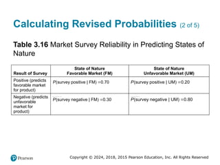
P, left parenthesis, unfavorable market, left parenthesis, U M, right parenthesis, vertical bar survey results positive, right parenthesis, equals 0.22. P, left parenthesis, favorable market, left parenthesis, F M, right parenthesis, vertical bar survey results negative, right parenthesis, equals 0.27. P, left parenthesis, unfavorable market, left parenthesis, U M, right parenthesis, vertical bar survey results negative, right parenthesis, equals 0.73.
#58 Long Description:
Two data tables, Probability Revisions Given a Positive Survey and Probability Revisions Given a Negative Survey, appear on the screen. Probability Revisions for a positive survey are calculated at 0.45, while Probability Revisions for a negative survey are calculated at 0.55.
Each probability revision table consists of five columns of four rows each.
The Probability Revisions Given a Positive Survey table is as follows,
Column A, descending,
State of Nature
F M
U M
Column B, descending,
P left parenthesis Sur. Pos.
0.7
0.2
Column C, descending,
Prior Prob.
0.5
0.5
P left parenthesisSur.pos right parenthesis equals
Column D, descending,
Joint Prob.
0.35
0.1
0.45 appears in bold text
Column E, descending,
Posterior Probability
0.78
0.22
Blank cell
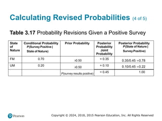
The Probability Revisions Given a Negative Survey table is as follows,
Column A, descending,
State of Nature
F M
U M
Column B, descending,
P left parenthesis Sur. Pos.
0.3
0.8
Column C, descending,
Prior Prob.
0.5
0.5
P left parenthesisSur.neg right parenthesis equals
Column D, descending,
Joint Prob.
0.15
0.4
0.55 appears in bold text
Column E, descending,
Posterior Probability
0.27
0.73
Blank cell
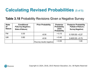
#59 Long Description:
The first row of the screenshot reads, from left to right, 0.7, 0.5, equals B 7 times C 7, equals D 7 forward slash dollar sign D dollar sign 9
The second row reads 0.2, equals 1 minus C 7, equals B 8 times C 8, equals D 8 forward slash dollar sign D dollar sign 9
The third row reads Blank cell, P left parenthesis Sur.pos. right parenthesis equals, equals SUM left parenthesis D 7 colon D 8 right parenthesis
The fourth and fifth rows are blank.
The sixth row reads P left parenthesis Sur. Pos. state of, Prior Prob., Joint Prob., and Posterior Probability
The seventh row reads = 1 minus B 7, equals C 7, equals B 13 times C 13, equals D 13 forward slash dollar sign D dollar sign 15
The eighth row reads equals 1 minus B 8, equals C 8, equals B 14 times C 14, equals D 14 forward slash dollar sign D dollar sign 15
The ninth row reads Blank cell, P left parenthesis Sur. neg. right parenthesis equals, equals SUM left parenthesis D 13 colon D 14 right parenthesis
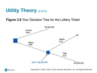
#62 Long Description:
The Reject Offer branch ends in a state of nature node labeled E M V equals two million, five hundred dollars. That node branches into a Heads left parenthesis 0.5 right parenthesis branch with zero dollars appearing at the end and a Tails left parenthesis 0.5 right parenthesis branch with five million dollars appearing at the end.
#63 Expected utility of alternative 2 = Expected utility of alternative 1
Utility of other outcome = p×(utility of best outcome, which is 1) + (1-p)×(utility of worst outcome, which is 0)
Utility of other outcome = p×(1)+(1-p)×0 = p
Long Description:
The Alternative 1 branch ends in a state of nature node, two branches stem from it, left parenthesis p right parenthesis that ends with the text Best Outcome Utility equals 1 and left parenthesis 1 minus p right parenthesis that ends with the text Worst Outcome Utility equals zero. The Alternative 2 branch ends with the text Other Outcome Utility equals question mark.
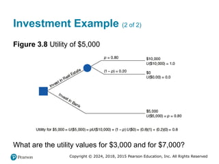
#65 Assess other utility values:
Utility for $7,000 = 0.9
Utility for $3,000 = 0.5
Use the three different dollar amounts and assess utilities.
Long Description:
Along the bottom of the diagram is the following equation, Utility for five thousand dollars equals U times five thousand dollars equals the product of p times U times ten thousand dollars the whole added to the product of 1 minus p times U times zero dollars equals the sum of 0.8 times 1and 0.2 times zero equals 0.8. The first branch extending from the decision node is labeled Invest in Real Estate. There is a state of nature node at the end, it branches into the following,
P equals 0.80 which results in ten thousand dollars, U times ten thousand dollars equals 1.0
Left parenthesis 1 minus p right parenthesis equals 0.20 which results in zero dollars, U times 0 dollars equals 0.0
The second branch extending from the decision node is labeled Invest in Bank. It ends with the data five thousand dollars, U times five thousand dollars equals p equals 0.80
#66 Long Description:
The line graph has Monetary Value, ranging from zero to ten thousand dollars in increments of one thousand, on the horizontal axis and Utility, ranging from zero to 1.0 in increments of 0.1, on the vertical axis, plots the following data, U times zero dollars equals zero, U times three thousand dollars equals 0.50, U times five thousand dollars equals 0.80, U times seven thousand dollars equals 0.90, and U times ten thousand dollars equals 1.0. The graph starts at ($0, 0), rises through ($3,000, 0.5), ($5,000, 0.80), ($7,000, 0.90), ($10,000, 1.0).
#67 Long Description:
A straight line bisects the graph area into two triangular halves, the top area shows a curved line bending downward toward the bisector and is labeled Risk Avoider. The bottom area shows a curved line bending upward toward the bisector and is labeled Risk Seeker. The bisecting line is labeled Risk Indifference.
#68 Long Description:
Alternative 1 Mark plays the game come to a state of nature node with two additional branches, Tack lands point up left parenthesis 0.45 right parenthesis which would yield ten thousand dollars, and Tack lands point down left parenthesis 0.55 right parenthesis which would yield negative ten thousand dollars. Alternative 2 Mark does not play the game would result in zero dollars.
#69 Long Description:
Utility is plotted on the vertical axis, ranging from zero to 1.00 in the following increments, 0.05, 0.15, 0.25, 0.30, 0.50, 0.75, and 1.00. The line curves up and to the right, crossing the following intersections, ten thousand dollars and 0.05, zero dollars and 0.15, ten thousand dollars and 0.30. The graph starts at ($ negative 20,000, 0), and rises through (negative 10,000, 0.05), ($0, 0.15), ($10,000, 0.30) to the first quadrant.
#70 Long Description:
Utility values have been added to each branch of the tree. Tack Lands Point Up has a utility of 0.30, Tack Lands Point Down has a utility of 0.05, and Don’t Play has a utility of 0.15. There is a pair of slash lines through the Don’t Play branch.


![[DSC Europe 25] Stefan Brankovic - #ResumeIsDead. AI-Powered Interviews and C...](https://cdn.slidesharecdn.com/ss_thumbnails/qnmbsv0xq3uysdrq3sev-2-stefan-brankovic-job-bolt-260114111931-a065aa3d-thumbnail.jpg?width=640&height=640&fit=bounds)


![[DSC Europe 25] Ivan Lukovic & Marija Djukic - From Data to Value: Why Maturi...](https://cdn.slidesharecdn.com/ss_thumbnails/ahrfps8xr6knowwhacxh-1-ivan-marija-dsc-2025-ld-v1-presentation-260115093812-be21adfc-thumbnail.jpg?width=640&height=640&fit=bounds)


![[DSC Europe 25] Slobodan Dolinic - Smart and Intelligent Green Region.pptx](https://cdn.slidesharecdn.com/ss_thumbnails/0bribinjsp6ghwtvsvor-2-sigre-slobodan-dolinic-260115093812-c9c10e90-thumbnail.jpg?width=640&height=640&fit=bounds)


