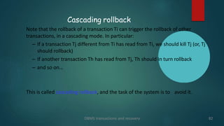
The document discusses transaction management and recovery management in database management systems. It begins by defining a schedule as an ordering of transactions' operations and characterizes schedules based on recoverability and serializability. It then discusses lock-based protocols, including two-phase locking and its pitfalls like deadlocks. Timestamp-based protocols are also covered. Validation-based optimistic concurrency control is defined with its three phases of read, validation, and write. The document concludes by discussing multiple granularity locking.


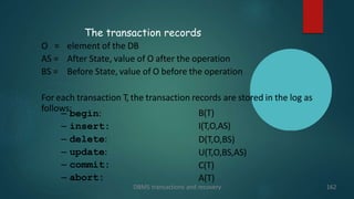
![New rules for the use of timestamps
DBMS transactions and recovery 142
The scheduler uses suitable data structures:
– For each version Xi the scheduler maintains a range range(Xi) = [wts, rts], where wts is
the timestamp of the transaction that wrote Xi, and rts is the highest timestamp
among those of the transactions that read Xi (if no one read Xi, then rts=wts).
– We denote with ranges(X) the set:
{ range(Xi) | Xi is a version of X }
– When ri(X) is processed, the scheduler uses ranges(X) to find the version Xj such that
range(Xj) = [wts, rts] has the highest wts that is less than or equal to the timestamp
ts(Ti) of Ti. Moreover, if ts(Ti) > rts, then the rts of range(Xj) is set to ts(Ti).
– When wi(x) is processed, the scheduler uses ranges(X) to find the version Xj such that
range(Xj) = [wts, rts] has the highest wts that is less than or equal to the timestamp
ts(Ti) of Ti. Moreover, if rts > ts(Ti), then wi(X) is rejected, else wi(Xi) is accepted, and
the version Xi with range(Xi) = [wts, rts], with wts = rts = ts(Ti) is created.](https://image.slidesharecdn.com/recoverability-240108054432-97b3ec76/85/db-unit-4-dbms-protocols-in-transaction-142-320.jpg)