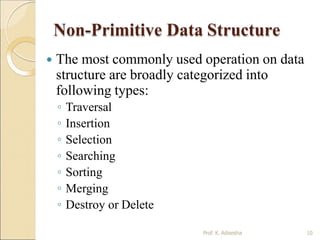
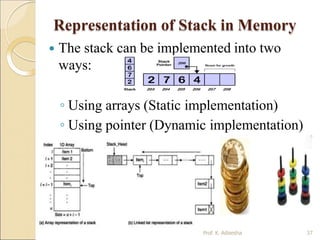
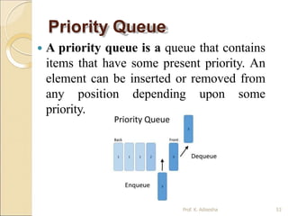
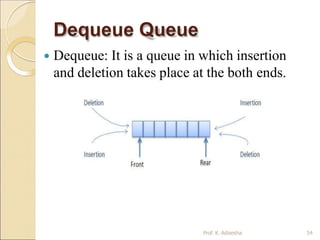
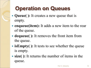
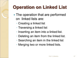
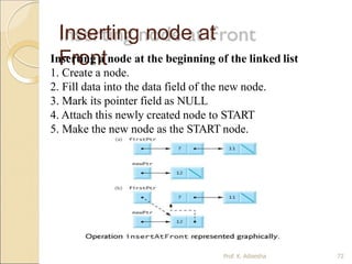
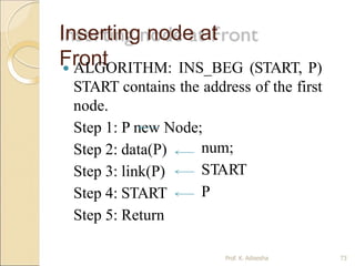
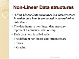
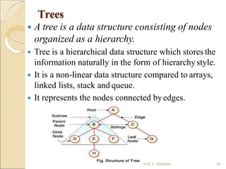
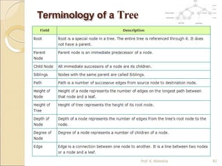
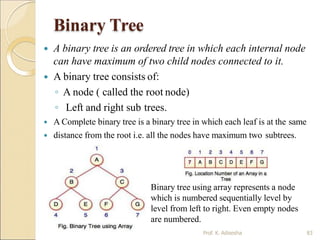
This document provides an introduction to data structures presented by Prof. K. Adisesha. It defines data structures as representations of logical relationships between data elements that consider both the elements and their relationships. Data structures affect both structural and functional aspects of programs. They are classified as primitive or non-primitive, with primitive structures operated on directly by machine instructions and non-primitive structures derived from primitive ones. Linear data structures like stacks and queues have elements in sequence, while non-linear structures like trees and graphs have hierarchical or parent-child relationships. Common operations on data structures include traversal, insertion, selection, searching, sorting, merging, and deletion. Arrays are also discussed in detail as a fundamental data structure.
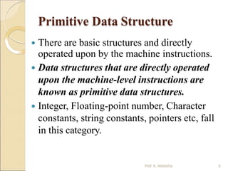
![One dimensional array:
Prof. K. Adisesha 13
An array with only one row or column is called one-dimensional
array.
It is finite collection of n number of elements of same type such
that:
◦ can be referred by indexing.
◦ The syntax Elements are stored in continuous locations.
◦ Elements x to define one-dimensional array is:
Syntax: Datatype Array_Name [Size];
Where,
Datatype : Type of value it can store (Example: int, char, float)
Array_Name: To identify the array.
Size : The maximum number of elements that the array can hold.](https://image.slidesharecdn.com/datastructureppt-1903271743401-230813114653-bf1a824b/85/datastructureppt-190327174340-1-pptx-13-320.jpg)
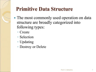
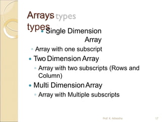
![Arrays
Prof. K. Adisesha 14
Simply, declaration of array is as follows:
int arr[10]
Where int specifies the data type or type of
elements arrays stores.
“arr” is the name of array & the number
specified inside the square brackets is the
number of elements an array can store, this is
also called sized or length of array.](https://image.slidesharecdn.com/datastructureppt-1903271743401-230813114653-bf1a824b/85/datastructureppt-190327174340-1-pptx-14-320.jpg)
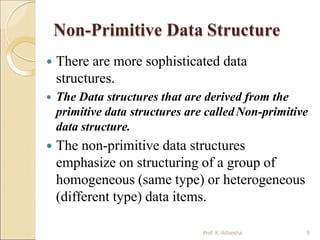
![Arrays
Prof. K. Adisesha 16
◦ The elements of array will always be stored in the
consecutive (continues) memory location.
◦ The number of elements that can be stored in an
array, that is the size of array or its length isgiven
by the following equation:
(Upperbound-lowerbound)+1
◦ For the above array it would be (9-0)+1=10,where 0
is the lower bound of array and 9 is the upper bound
of array.
◦ Array can always be read or written through loop.
For(i=0;i<=9;i++)
{ scanf(“%d”,&arr[i]);
printf(“%d”,arr[i]); }](https://image.slidesharecdn.com/datastructureppt-1903271743401-230813114653-bf1a824b/85/datastructureppt-190327174340-1-pptx-16-320.jpg)
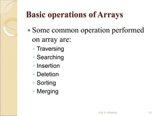
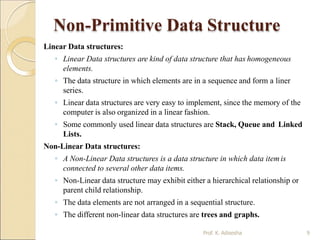
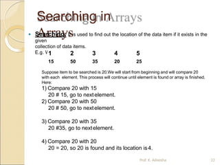
![Traversing
Arrays
Traversing: It is used to access each data item exactly
once so
that it can be processed.
E.g.
We have linear array A as below:
1 2 3 4 5
10 20 30 40 50
Here we will start from beginning and will go till last element
and during this process we will access value of each
element exactly once as below:
A [1] = 10
A [2] = 20
A [3] = 30
A [4] = 40
A [5] = 50
Prof. K. Adisesha 19](https://image.slidesharecdn.com/datastructureppt-1903271743401-230813114653-bf1a824b/85/datastructureppt-190327174340-1-pptx-19-320.jpg)
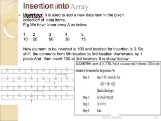
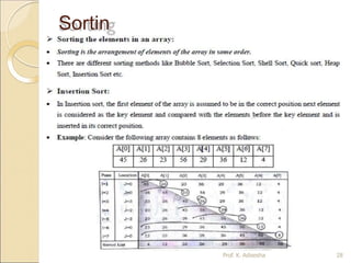
![Insertion Sort
ALGORITHM: Insertion Sort (A, N)A is an array with N
unsorted elements.
◦ Step 1: for I=1 to N-1
◦ Step 2: J = I
While(J >= 1)
if ( A[J] < A[J-1]) then
Temp = A[J];
A[J] = A[J-1];
A[J-1] =
Temp;
[End if]
J = J-1
[End of While
loop] [End of For
loop]
◦ Step 3: Exit Prof. K. Adisesha 29](https://image.slidesharecdn.com/datastructureppt-1903271743401-230813114653-bf1a824b/85/datastructureppt-190327174340-1-pptx-29-320.jpg)
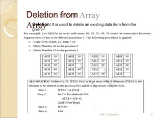
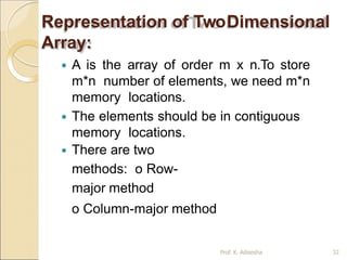
![Two dimensional
array
Prof. K. Adisesha 31
A two dimensional array is a collection of elements and
each element is identified by a pair of subscripts. ( A[3]
[3] )
The elements are stored in continuous memory
locations.
The elements of two-dimensional array as rows and
columns.
The number of rows and columns in a matrix is called
as
the order of the matrix and denoted as mxn.
The number of elements can be obtained by
multiplying
number of rows and number of columns.
A[0] A[1] A[2]
A[0] 10 20 30
A[1] 40 50 60
A[2] 70 80 90](https://image.slidesharecdn.com/datastructureppt-1903271743401-230813114653-bf1a824b/85/datastructureppt-190327174340-1-pptx-31-320.jpg)
![Two Dimensional Array:
Prof. K. Adisesha 33
Row-Major Method: All the first-row elements are stored in
sequential memory locations and then all the second-row
elements are stored and so on. Ex:A[Row][Col]
Column-Major Method: All the first column elements are
stored in sequential memory locations and then all the second-
column elements are stored and so on. Ex: A[Col][Row]
1000 10 A[0][0]
1002 20 A[0][1]
1004 30 A[0][2]
1006 40 A[1][0]
1008 50 A[1][1]
1010 60 A[1][2]
1012 70 A[2][0]
1014 80 A[2][1]
1016 90 A[2][2]
Row-Major Method
1000 10 A[0][0]
1002 40 A[1][0]
1004 70 A[2][0]
1006 20 A[0][1]
1008 50 A[1][1]
1010 80 A[2][1]
1012 30 A[0][2]
1014 60 A[1][2]
1016 90 A[2][2]
Col-Major Method](https://image.slidesharecdn.com/datastructureppt-1903271743401-230813114653-bf1a824b/85/datastructureppt-190327174340-1-pptx-33-320.jpg)
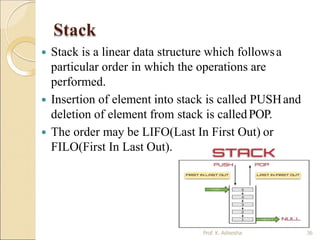
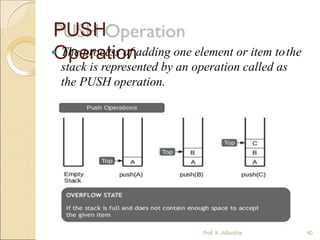
![PUSH
Operation:
Prof. K. Adisesha 41
The process of adding one element or item to the stack is
represented by an operation called as the PUSH operation.
The new element is added at the topmost position of the stack.
ALGORITHM:
PUSH (STACK, TOP, SIZE, ITEM)
STACK is the array with N elements. TOP is the pointer to the top of the
element of the array. ITEM to be inserted.
Step 1: if TOP = N then [Check Overflow]
PRINT “ STACK is Full or Overflow”
Exit
[Increment the TOP]
[Insert the ITEM]
[End if]
Step 2: TOP = TOP +1
Step 3: STACK[TOP] = ITEM
Step 4: Return](https://image.slidesharecdn.com/datastructureppt-1903271743401-230813114653-bf1a824b/85/datastructureppt-190327174340-1-pptx-41-320.jpg)
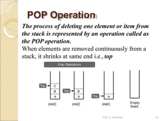
![POP Operation
Prof. K. Adisesha 43
The process of deleting one element or item from the stack
is represented by an operation called as the POP
operation.
ALGORITHM: POP (STACK, TOP, ITEM)
STACK is the array with N elements. TOP is the pointer to the top of the
element of the array. ITEM to be inserted.
Step 1: if TOP = 0 then [Check Underflow]
PRINT “ STACK is Empty or Underflow”
Exit
[End if]
[copy the TOPElement]
[Decrement the TOP]
Step 2: ITEM = STACK[TOP]
Step 3: TOP = TOP -1
Step 4: Return](https://image.slidesharecdn.com/datastructureppt-1903271743401-230813114653-bf1a824b/85/datastructureppt-190327174340-1-pptx-43-320.jpg)
![PEEK
Operation
Prof. K. Adisesha 44
The process of returning the top item from the
stack but does not remove it called as the POP
operation.
ALGORITHM: PEEK (STACK, TOP)
STACK is the array with N elements. TOP is the pointer to
the top of the element of the array.
Step 1: if TOP = NULL then [Check Underflow]
PRINT “ STACK is Empty or Underflow”
Exit
[End if]
Step 2: Return (STACK[TOP] [Return the top
element of the stack]
Step 3:Exit](https://image.slidesharecdn.com/datastructureppt-1903271743401-230813114653-bf1a824b/85/datastructureppt-190327174340-1-pptx-44-320.jpg)
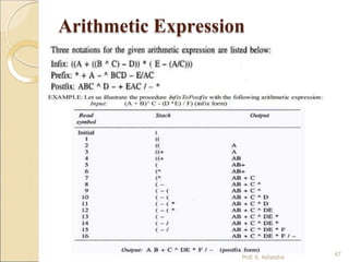
![Arithmetic Expression
Example: +ab
Prof. K. Adisesha 46
An expression is a combination of operands and operators
that after evaluation results in a single value.
· Operand consists of constants and variables.
· Operators consists of {, +, -, *, /, ), ] etc.
Expression can be
Infix Expression: If an operator is in between two operands, it is called
infix expression.
Example: a + b, where a and b are operands and + is an operator.
Postfix Expression: If an operator follows the two operands, it is called
postfix expression.
Example: ab +
Prefix Expression: an operator precedes the two operands, it is called
prefix expression.](https://image.slidesharecdn.com/datastructureppt-1903271743401-230813114653-bf1a824b/85/datastructureppt-190327174340-1-pptx-46-320.jpg)
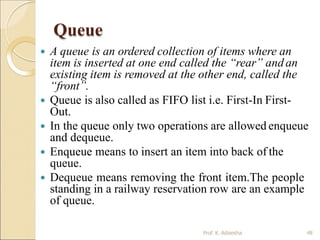
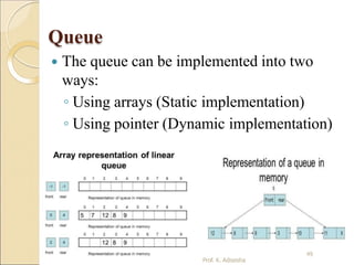
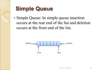
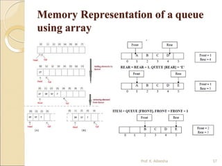
![Queue Insertion Operation
(ENQUEUE):
ALGORITHM: ENQUEUE (QUEUE, REAR, FRONT, ITEM)
QUEUE is the array with N elements. FRONT is the pointer that contains the
location of the element to be deleted and REAR contains the location of the
inserted element. ITEM is the element to be inserted.
Step 1: if REAR = N-1 then [Check Overflow]
PRINT “QUEUE is Full or Overflow”
Exit
[End if]
Step 2: if FRONT = NULL then [Check Whether Queue isempty]
FRONT = -1
REAR = -1
else
REAR = REAR + 1 [Increment REAR Pointer]
Step 3: QUEUE[REAR] = ITEM [Copy ITEM to REAR position]
Step 4: Return
Prof. K. Adisesha 58](https://image.slidesharecdn.com/datastructureppt-1903271743401-230813114653-bf1a824b/85/datastructureppt-190327174340-1-pptx-58-320.jpg)
![Queue Deletion Operation
(DEQUEUE)
ALGORITHM: DEQUEUE (QUEUE, REAR, FRONT, ITEM)
QUEUE is the array with N elements. FRONT is the pointer that contains the
location of the element to be deleted and REAR contains the location of the
inserted element. ITEM is the element to be inserted.
Step 1: if FRONT = NULL then [Check Whether Queue isempty]
PRINT “QUEUE is Empty or Underflow”
Exit
[End if]
Step 2: ITEM = QUEUE[FRONT]
Step 3: if FRONT = REAR then [if QUEUE has only one element]
FRONT = NULL
REAR = NULL
else
FRONT = FRONT + 1 [Increment FRONT pointer]
Step 4: Return
Prof. K. Adisesha 59](https://image.slidesharecdn.com/datastructureppt-1903271743401-230813114653-bf1a824b/85/datastructureppt-190327174340-1-pptx-59-320.jpg)

![Operator new and delete
Prof. K. Adisesha 69
Operators new allocate memory
space.
◦ Operators new [ ] allocates memory
space for array.
Operators delete deallocate
memory space.
◦ Operators delete [ ] deallocate
memory space for array.](https://image.slidesharecdn.com/datastructureppt-1903271743401-230813114653-bf1a824b/85/datastructureppt-190327174340-1-pptx-69-320.jpg)
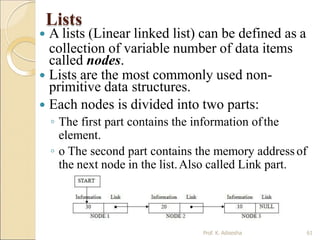
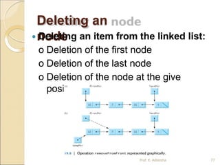
![Traversing a linked list:
Prof. K. Adisesha 70
Traversing is the process of accessing each node of the
linked list exactly once to perform some operation.
ALGORITHM: TRAVERS (START, P) START contains
the address of the first node. Another pointer p is
temporarily used to visit all the nodes from the beginning to
the end of the linked list.
Step 1: P = START
Step 2: while P != NULL
Step 3:
Step 4:
PROCESS data (P)
P = link(P)
[Fetch the data]
[Advance P to next node]
Step 5: End of while
Step 6: Return](https://image.slidesharecdn.com/datastructureppt-1903271743401-230813114653-bf1a824b/85/datastructureppt-190327174340-1-pptx-70-320.jpg)
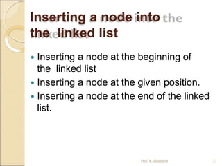
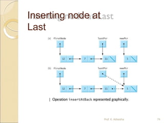
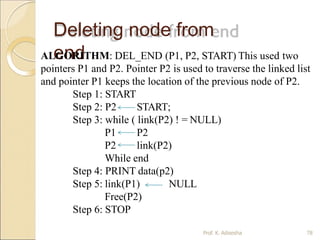
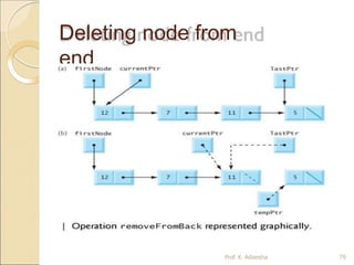
![Inserting node at
Last
ALGORITHM: INS_END (START, P) START contains
the address of the first node.
Step 1: START
Step 2: P START [identify the last node]
while P!= null
P next (P)
End while
Step 3: N new Node;
Step 4: data(N) item;
Step 5: link(N) null
Step 6: link(P) N
Step 7: Return Prof. K. Adisesha 75](https://image.slidesharecdn.com/datastructureppt-1903271743401-230813114653-bf1a824b/85/datastructureppt-190327174340-1-pptx-75-320.jpg)
![Inserting node at a given
Position
count+1
next (P)
Count 0
Step 3: while P!= null
count
P
End while
Step 4: if (POS=1)
Call function INS_BEG( )
else if (POS=Count +1)
Call function INS_END( )
For(i=1; i<=pos; i++)
P next(P);
end for
new node
item;
link(P)
N
[create] N
data(N)
link(N)
link(P)
else
PRINT “Invalid position”
Step 5: Return
ALGORITHM: INS_POS (START, P) START contains the
address of the first node.
Step 1: START else if (POS<=Count)
Step 2: P START [Initialize node] P Start
Prof. K. Adisesha 76](https://image.slidesharecdn.com/datastructureppt-1903271743401-230813114653-bf1a824b/85/datastructureppt-190327174340-1-pptx-76-320.jpg)
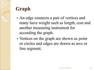
![Graph
Example of graph:
v2
v1
v5
v3
10
15
8
6
11
9
v4
v1
v2 v4
v3
[a] Directed &
Weighted Graph Prof. K. Adisesha 85
[b] Undirected Graph](https://image.slidesharecdn.com/datastructureppt-1903271743401-230813114653-bf1a824b/85/datastructureppt-190327174340-1-pptx-85-320.jpg)