BCS304 Module 5 slides DSA notes 3rd sem

SIR M VISVESVARAYA INSTITUTE OF TECHNOLOGY
Krishnadevarayanagar, Hunasamaranahalli, Yelahanka, International
Airport Road, Bengaluru - 562 157
Data Structures and Applications
BCS304

Syllabus
Department of CSE 2
Module – 1
INTRODUCTION TO DATA STRUCTURES: Data Structures, Classifications (Primitive & Non-Primitive),
Data structure Operations, Review of pointers and dynamic Memory Allocation,
ARRAYS and STRUCTURES: Arrays, Dynamic Allocated Arrays, Structures and Unions, Polynomials,
Sparse Matrices, representation of Multidimensional Arrays, Strings
STACKS: Stacks, Stacks Using Dynamic Arrays, Evaluation and conversion of Expressions
Text Book: Chapter-1:1.2 Chapter-2: 2.1 to 2.7 Chapter-3: 3.1,3.2,3.6
Reference Book 1: 1.1 to 1.4 8 Hours
Module – 2
QUEUES: Queues, Circular Queues, Using Dynamic Arrays, Multiple Stacks and queues.
LINKED LISTS : Singly Linked, Lists and Chains, Representing Chains in C, Linked Stacks and
Queues, Polynomials
Text Book: Chapter-3: 3.3, 3.4, 3.7 Chapter-4: 4.1 to 4.4

Syllabus
Department of CSE 3
Module – 3
LINKED LISTS : Additional List Operations, Sparse Matrices, Doubly Linked List.
TREES: Introduction, Binary Trees, Binary Tree Traversals, Threaded Binary Trees.
Text Book: Chapter-4: 4.5,4.7,4.8 Chapter-5: 5.1 to 5.3, 5.5 8 Hours
Module – 4
TREES(Cont..): Binary Search trees, Selection Trees, Forests, Representation of Disjoint sets,
Counting Binary Trees,
GRAPHS: The Graph Abstract Data Types, Elementary Graph Operations
Text Book: Chapter-5: 5.7 to 5.11 Chapter-6: 6.1, 6.2
Module – 5
HASHING: Introduction, Static Hashing, Dynamic Hashing
PRIORITY QUEUES: Single and double ended Priority Queues, Leftist Trees
INTRODUCTION TO EFFICIENT BINARY SEARCH TREES: Optimal Binary Search Trees
Text Book: Chapter 8: 8.1 to 8.3 Chapter 9: 9.1, 9.2 Chapter 10: 10.1

Textbook and References
Department of CSE 4
Textbooks:
1. Ellis Horowitz and Sartaj Sahni, Fundamentals of Data Structures in C, 2nd Ed, Universities Press,
2014.
Reference Books:
1. Seymour Lipschutz, Data Structures Schaum's Outlines, Revised 1st Ed, McGraw Hill,2014.
Cengage
2. Gilberg & Forouzan, Data Structures: A Pseudo-code approach with C, 2nd
Ed, Learning,2014.
3. Reema Thareja, Data Structures using C, 3rd Ed, Oxford press, 2012.
4. Jean-Paul Tremblay & Paul G. Sorenson, An Introduction to Data Structures with Applications, 2nd
Ed, McGraw Hill, 2013
5. A M Tenenbaum, Data Structures using C, PHI, 1989
6. Robert Kruse, Data Structures and Program Design in C, 2nd Ed, PHI, 1996.

COURSE OBJECTIVE
Department of CSE 5
After studying this course, students will be able
to: Course Learning Objective
1. To explain fundamentals of data structures and
their applications.
2. To illustrate representation of Different data structures such as Stack, Queues,
LinkedLists, Trees and Graphs.
3.
4.
5. and Optimal
To Design and Develop Solutions to problems using Linear Data Structures.
To discuss applications of Nonlinear Data Structures in problem solving.
To introduce advanced Data structure concepts such as Hashing
BinarySearch Trees

COURSE OUTCOMES
Department of CSE 6
After studying this course, students will be able
to: Course Outcomes
1. Explain different data structures and their
applications.
2. Apply Arrays, Stacks and Queue data structures to
solve the given problems.
3.
4.
5.
Use the concept of linked list in problem solving.
Develop solutions using trees and graphs to model the real-world problem.
Explain the advanced Data Structures concepts such as Hashing Techniques and
Optimal Binary Search Trees.

HASHING: Introduction, Static Hashing, Dynamic Hashing
PRIORITY QUEUES: Single and double ended Priority Queues, Leftist Trees
INTRODUCTION TO EFFICIENT BINARY SEARCH TREES: Optimal Binary
Search Trees
Text Book: Chapter 8: 8.1 to 8.3 Chapter 9: 9.1, 9.2 Chapter 10: 10.1
8 Hours
Department of CSE 7
Module – 5

Additional Operations on Linked List
Department of CSE 8
1. Inserting an element at a given position
2. Inserting an element after a given position
3. Inserting an element before a given position
4. Inserting an element before Key Element
5. Inserting an element after the key element
6. Ordered Inserting into a list
7. Deleting a key element
8. Deleting an element at a given position
9. Reverse a linked list
10. Concatenation of two linked list
11. Count the number of nodes in a list

Hashing
Department of CSE 9
The Symbol Table Abstract Data Type
Static Hashing
Hash Tables
Hashing Functions
Mid-square
Division
Folding
Digit Analysis
Overflow Handling
Linear Open Addressing, Quadratic probing,
Rehashing Chaining

The Symbol Table ADT
Department of CSE 10
• Many example of dictionaries are found in many applications, Ex.
spelling checker
• In computer science, we generally use the term symbol table rather
than dictionary, when referring to the ADT.
• We define the symbol table as a set of name-attribute pairs.
• Example: In a symbol table for a compiler
• the name is an identifier
• the attributes might include an initial value
• a list of lines that use the identifier.

• Operations on symbol table:
• Determine if a particular name is in the table
• Retrieve/modify the attributes of that name
• Insert/delete a name and its attributes
• Implementations
• Binary search tree: the complexity is O(n)
• Some other binary trees (chapter 10): O(log n).
• Hashing
• A technique for search, insert, and delete operations that
has very good expected performance.

Search Techniques
• Hashing methods
• Relies on a formula called the hash function.
• Types of hashing
• Static hashing
• In• stDatyicnahmasichihnags,hwineg store the identifiers in a fixed size
table called a
hash table
• Arithmetic function, f
• To determine the address of an identifier, x, in the table
• f(x) gives the hash, or home address, of x in the table
• Hash table, ht

Hash Tables

Hash Tables
• The identifier density of a hash table
is the ratio n/T
• n is the number of identifiers in the
table
• T is possible identifiers
• The loading density or loading
factor
of a hash table is α = n/(sb)
• s is the number of slots
• b is the number of buckets

Hash Tables
1 2 1 2
• Two identifiers, i and i are synonyms with respect to f if f(i ) =
f(i )
• We enter distinct synonyms into the same bucket as long as the bucket has
slots available
• An overflow occurs when we hash a new identifier into a full bucket
• A collision occurs when we hash twonon-identical identifiers into the same
bucket.
• When the bucket size is 1, collisions and overflows occur simultaneously.
• Example 8.1: Hash table
• b = 26 buckets and s = 2 slots. Distinct identifiers n = 10
• The loading factor, is 10/52 = 0.19.
• Associate the letters, a-z, with the numbers , 0-25, respectively

Hash Tables
• The time required to enter, delete, or search for identifiers does not depend on
the number of identifiers n in use; Hash function requirements:
• Easy to compute and produces few collisions.
• Unfortunately, since the ration b/T is usually small, we cannot avoid collisions
altogether.
=> Overload handling mechanisms are needed
C library functions (f(x)):
acos(0), define(3), float(5), exp(4), char(2),
atan(0), ceil(2), floor(5), clock(2), ctime(2)
overflow: clock, ctime

Hashing Functions
• A hash function, f, transforms an identifier, x, into a bucket address in the hash
table.
• We want a hash function that is easy to compute and that minimizes the
number of collisions.
• Hashing functions should be unbiased.
• That is, if we randomly choose an identifier, x, from the identifier space, the
probability that f(x) = i is 1/b for all buckets i.
• We call a hash function that satisfies unbiased property a
uniform hash function.
Mid-square, Division, Folding, Digit Analysis

Hashing Functions - Mid-square
• Mid-square f (x)=middle(x2
):
m
• Frequently used in symbol table applications.
• We compute fm
by squaring the identifier and then using an appropriate
number of bits from the middle of the square to obtain the bucket
address.
• The number of bits used to obtain the bucket address depends on the table
size. If we use r bits, the range of the value is 2r
.
• Since the middle bits of the square usually depend upon all the characters in
an identifier, there is high probability that different identifiers will
produce different hash addresses.

Hashing Functions - Division
• Division fD
(x) = x % M :
• Using the modulus (%) operator.
• We divide the identifier x by some number M and use the remainder as
the hash address for x.
• This gives bucket addresses that range from 0 to M - 1, where M = that
table size.
• The choice of M is critical.
• If M is divisible by 2, then odd keys to odd buckets and even keys
to even buckets. (biased!!)

Hashing Functions - Division (Cont..)
The choice of M is critical (cont’d)
• When many identifiers are permutations of each other, a biased use of the table
results.
• Example: X=x1
x2
and Y=x2
x1
Internal binary representation: x1
--> C(x1
) and x2
--> C(x2
)
Each character is represented by six bits
1 2 2 1
X: C(x ) * 26
+ C(x ), Y: C(x ) * 26
+ C(x )
(fD
(X) - fD
(Y)) % p (where p is a prime number)
1 2 2 1
= (C(x ) * 26
% p + C(x ) % p - C(x ) * 26
% p - C(x ) % p ) % p
6
p = 3, 2 =64
(64 % 3 * C(x1
) % 3 + C(x2
) % 3 - 64 % 3 * C(x2
) % 3 - C(x1
) % 3) % 3
= C(x1
) % 3 + C(x2
) % 3 - C(x2
) % 3 - C(x1
) % 3 = 0 % 3
The same behavior can be expected when p = 7
• A good choice for M would be : M a prime number such that M does not divide rk
±a
for small k and a.

Hashing Functions - Folding
Folding
• Partition identifier x into several parts
• All parts except for the last one have the same length
• Add the parts together to obtain the hash address
• Two possibilities (divide x into several parts)
• Shift folding:
Shift all parts except for the last one, so that the least significant bit
of each part lines up with corresponding bit of the last part.
x1
=123, x2
=203, x3
=241, x4
=112, x5
=20, address=699
• Folding at the boundaries:
reverses every other partition before adding
x1
=123, x2
=302, x3
=241, x4
=211, x5
=20, address=897

Hashing Functions - Folding
P1 P2 P3 P4 P5
20
shift folding 123
203
241
1
1
2
2
0
699
folding at the
boundaries
MSD ---> LSD
LSD <--- MSD
123 203 241 112 20
Folding example:
123
203
241
112

Hashing Functions - Digit Analysis
Digit Analysis
• Used with static files
• A static files is one in which all the identifiers are known in advance.
• Using this method,
• First, transform the identifiers into numbers using some radix, r.
• Second, examine the digits of each identifier, deleting those digits that have
the most skewed distribution.
• We continue deleting digits until the number of remaining digits is small
enough to give an address in the range of the hash table.

Hashing Functions - Digit Analysis
Digital Analysis example:
All the identifiers are known in advance, M=1~999
d12
d22
…
…
X1
:d11
X2
:d21
…
dm2
Xm
:dm1
…
d1n
d2n
dm
n
Select 3 digits from n
Criterion: Delete the digits having the most skewed distributions
• The one most suitable for general purpose applications is the division method
with a divisor, M, such that M has no prime factors less than 20.

Overflow Handling - Linear probing
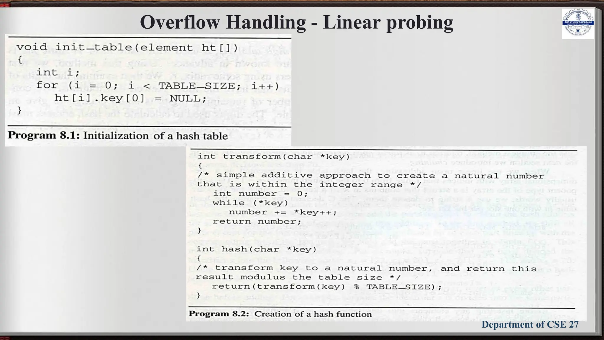
Linear open addressing (Linear probing)
• Compute f(x) for identifier x
• Examine the buckets:
ht[(f(x)+j)%TABLE_SIZE], 0 ≤ j ≤ TABLE_SIZE
• The bucket contains x.
• The bucket contains the empty string (insert to it)
• The bucket contains a nonempty string other than x
(examine the next bucket) (circular rotation)
• Return to the home bucket ht[f(x)],
if the table is full we report an error condition and
exit

Additive transformation and Division
Hash table with linear probing (13 buckets, 1 slot/bucket)

Overflow Handling - Problem of Linear Probing
Problem of Linear Probing
• Identifiers tend to cluster together
• Adjacent cluster tend to coalesce
• Increase the search time
• Example: suppose we enter the C built-in
functions into a 26-bucket hash table in order.
The hash function uses the first character in
Hash table with linear probing (26 buckets, 1 slot/bucket)
Enter:
cfaacd
felltott
ehoxe
oiomo
aipafs
ollitsr
nree
Enter seeqacuhenfucnec:tion name
acos, atoi, char, define, exp,
ceil, cos, float, atol, floor, ctime
# of key
comparisons=35/11=3.18

Overflow Handling
• Alternative techniques to improve open addressing
approach:
• Quadratic probing
• rehashing
• random probing
• Rehashing
• Try f1
, f2
, …, fm
in sequence if collision occurs
• disadvantage
• comparison of identifiers with different hash values
• use chain to resolve collisions

Overflow Handling - Quadratic Probing
Prime j Prime j
3 0 43 10
7 1 59 14
11 2 127 31
19 4 251 62
23 5 503 125
31 7 1019 254
Quadratic Probing
• Linear probing searches buckets (f(x)+i)%b
• Quadratic probing uses a quadratic function of i as the increment
• Examine buckets f(x),
(f(x)+i2
)%b, (f(x)-i2
)%b, for 1<=i<=(b-1)/2
• When b is a prime number of the form 4j+3, j is an integer, the
Chaqiunaidnrgatic search examines every bucket in the table
• Linear probing and its variations perform poorly because inserting an identifier requires
the comparison of identifiers with different hash values.
• In this approach we maintained a list of synonyms for each bucket.
• To insert a new element
• Compute the hash address f (x)
• Examine the identifiers in the list for f(x).
• Since we would not know the sizes of the lists in advance, we should maintain them as
lined chains

Overflow Handling - Hash Chaining
Results of Hash Chaining
acos, atoi, char, define, exp,
ceil, cos, float, atol, floor,
ctime
f (x)=first character of x
# of key comparisons=21/11=1.91

Overflow Handling - Comparison
Comparison:
• In Figure 8.7, The values in each column give the average number of
bucket accesses made in searching eight different table with
33,575, 24,050, 4909, 3072, 2241, 930, 762, and 500 identifiers each.
• Chaining performs better than linear open addressing.
• We can see that division is generally superior

Dynamic Hashing-using directories
• simulation
• Dynamic hashing using directories
• Analysis of directory dynamic hashing
• Directoryless dynamic hashing

Dynamic Hashing Using Directories

Directoryless Dynamic Hashing

Thank You

BCS304 Module 5 slides DSA notes 3rd sem

More Related Content

What's hot

Similar to BCS304 Module 5 slides DSA notes 3rd sem

Recently uploaded

BCS304 Module 5 slides DSA notes 3rd sem