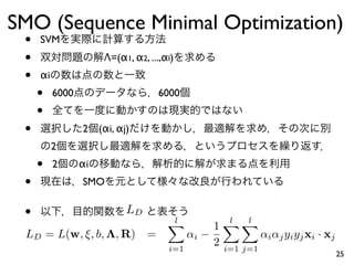
SlideShare a Scribd company logo
•          k-NN
         •             Yes, No


Training Data


 Test Data


                                 3
4
•                         xi                       yi      i
              1   -1
    (xi , yi )(i = 1, . . . , l, xi ∈ Rn , yi ∈ {1, −1})

•                  w, b
    yi (w · (xi − b)) > 0 (i = 0, . . . , l)


                                                           5
•                w.x+b≧0
•                 
                      1,
                           x      d(x)
                          if w · x + b ≥ 0
        d(x) =
                      −1, otherwise
•
    •


                                             6
Fisher            (1)
•                     2    2


    •          aw+b
    •   aw+b


                                7
Fisher                              (2)
•                  
                       m+ m-
                                              
                     d(x)=1   x                  d(x)=−1   x
         m+ =                     , m− =
                 |{x|d(x) = 1}|             |{x|d(x) = −1}|

•                      |(m+ − m− ) · w|
    •
•        
          w.x+b=0
                                    
                           2                               2
            ((x − m+ ) · w) +               ((x − m− ) · w)
        d(x)=1                    d(x)=−1


    •

                                                               8
Fisher                               (3)
•
•               |w|=1                J(w)                 w
    •                        w.x+b
    •   b
                                                2
                           |(m+ − m− ) · w|
    J(w) =                       2                        2
            d(x)=1 ((x − m+ ) · w) + d(x)=−1 ((x − m− ) · w)


                              J(w)          w
                              J(w)     w             0


                                                                9
Fisher                       (4)
 J(w)
          w T SB w
J(w)    =
          w T SW w
          SB = (m+ − m− )(m+ − m− )T
                                            
          SW =      (x − m+ )(x − m+ )T +             (x − m− )(x − m− )T
                   d(x)=1                   d(x)=−1
             ∂J(w)
           0       =0
              ∂w
          
          f     f  g − f g
              =
          g           g2

(wT SB w)SW w = (wT SW w)SB w
            2                          SB w  m+ − m−
 w ∝ S−1 (m+ − m− )
      W


                  Sw                                                  10
SVM (Support Vector Machine)
•
    •
•


                               11
•       ρ(w,b)
                         xi · w              xi · w
    ρ(w, b) =   min             − max
              {xi |yi =1} |w|    {xi |yi =−1} |w|


                                                      12
2/|w0 |
             w0         w0 · x + b0 ≥ 1


                                            w0 · x + b0 = 1
                                                w0 · x + b0 = 0
          w0 · x + b0 ≤ −1                w0 · x + b0 = −1


w0 · x + b0 = ±1                 w0, b0
                                      xi · w0               xi · w0
            ρ(w0 , b0 ) =   min                − max
                          {xi |yi =1} |w0 |     {xi |yi =−1} |w0 |
                          1 − b0       −1 − b0       2
                        =           −           =
                           |w0 |         |w0 |    |w0 |
                                                                      13
• 2/|w0 |               w0 · w0


            yi (w0 · xi + b) ≥ 1 (i = 1, . . . , l)

                      w0 · w0                  w0

•             2                 2
    •                                          2
    •             1
•   2


    •                                                 14
(1)
    yi (w0 · xi + b) ≥ 1 (i = 1, . . . , l)               (1)

            w0 · w0                    w0
       Λ = (α1 , . . . , αl ) (αi ≥ 0)
                                       l
                            |w|2 
       L(w, b, Λ)      =        −     αi (yi (xi · w + b) − 1)
                             2    i=1

•                             w, b                  Λ


                                                           15
(2)
•   w=w0, b=b0
                          
                                  L(w, b, Λ)
                                                              l
              ∂L(w, b, Λ)                                    
                                          =       w0 −             αi yi xi = 0
                 ∂w       
                             
                                 w=w0
                                                        l
                                                              i=1                  (2)
                 ∂L(w, b, Λ)                           
                                          =       −          αi yi = 0
                    ∂b       
                                  b=b0                  i=1
                          l
                                                  l
                                                   
                 w0 =           αi yi xi   ,             αi yi = 0
                          i=1                      i=1

•                         w=w0, b=b0
                                        l
                            1
       L(w0 , b0 , Λ) =       w0 · w0 −     αi [yi (xi · w0 + b0 ) − 1]
                            2           i=1
                            l
                                              l    l
                                     1 
                     =          αi −           αi αj yi yj xi · xj
                            i=1
                                     2 i=1 j=1

•                     w     b
                      Λ                                                                  16
SVM
•             l
              
                                  w, b
                    αi yi = 0, αi ≥ 0
              i=1                                                         (3)
                                 l
                                                 l   l
                                          1 
         L(w0 , b0 , Λ) =            αi −           αi αj yi yj xi · xj
                                 i=1
                                          2 i=1 j=1
                       Λ
•   SVM
•   w0                        Λ
                                  l
    •     (2)           ( w0 =          i=1   αi yi xi )
•       (2)         αi≠0           xi     w                KKKT


    •    KKT         : αi [yi (xi · w0 + b0 ) − 1] = 0
                                                                           17
•
•
•


    (A)   (B)   18
(       )
•
    •
    •
•
    •                        l
                                           l   l
                                       1 
        L(w0 , b0 , Λ) =          αi −           αi αj yi yj xi · xj
                              i=1
                                       2 i=1 j=1
    •    x
                         l
                         
                                Φ(x)
                                        l   l
                                  1 
        L(w0 , b0 , Λ) =     αi −           αi αj yi yj Φ(xi ) · Φ(xj )
                         i=1
                                  2 i=1 j=1
    •                            l
                                 
        Φ(x) · w0 + b0      =          αi yi Φ(x) · Φ(xi ) + b0 = 0
                                 i=1

    •             Φ
                                                                          19
Kernel
•            K(x, y) = Φ(x)
                              √
                                Φ(y)
                                           √     √
•       Φ((x1 , x2 )) = (x1 , 2x1 x2 , x2 , 2x1 , 2x2 , 1)
                           2             2

        Φ((x1 , x2 )) · Φ((y1 , y2 ))
          = (x1 y1 )2 + 2x1 y1 x2 y2 + (x2 y2 )2 + 2x1 y1 + 2x2 y2 + 1
          = (x1 y1 + x2 y2 + 1)2
          = ((x1 , x2 ) · (y1 , y2 ) + 1)2
    •                 (6     )
•
    •                         (x · y + 1)d ,
    •     RBF                 exp(−||x − y||2 /2σ 2 ),
    •                         tanh(κx · y − δ)
         •   σ κ   δ
         •                                                     Mercer
                                                                         20
•

•
    •
        •   ξ

yi (w · xi + b) ≥ 1 − ξi
  where ξi ≥ 0 (i = 1, . . . , l)

             l     
    1        
      w·w+C      ξi
    2        i=1

                                    21
(1)
         •
                               Λ = (α1 , . . . , αl ), R = (r1 , . . . , rl )
                   L
  L(w, ξ, b, Λ, R)
                        l
                                    l
                                                                                l
                                                                                 
         1
     =     w·w+C              ξi −         αi [yi (xi · w + b) − 1 + ξi ] −            ri ξi
         2              i=1          i=1                                         i=1

w0 , b0 , ξi L
           0
                               w, b, ξi                                KKT
                                                         l
                                                          
             ∂L(w, ξ, b, Λ, R) 
                               
                                            = w0 −             α i y i xi = 0
                   ∂w              w=w0                   i=0
                                                   l
                                                    
              ∂L(w, ξ, b, Λ, R) 
                                
                                            = −          αi yi = 0
                     ∂b
                                 b=b0              i=0
              ∂L(w, ξ, b, Λ, R) 
                                
                                 0          = C − αi − ri = 0
                    ∂ξi           ξ=ξ                                                          22
                                       i
(2)
•                                    l
                                     
                                             L
                                                 l
                                              1 
                                                     l
        L(w, ξ, b, Λ, R) =               αi −           αi αj yi yj xi · xj
                                              2 i=1 j=1
•
                                     i=1
                                                               C ξ
                                          SVM
    •                           αi            C
    •   C
•   C - αi - ri = 0        ri                                0≦αi≦C

                l
                                    w,b
                
                      αi yi = 0, 0 ≤ αi ≤ C
                i=1

                                     l
                                                 l    l
                                              1 
        L(w, ξ, b, Λ, R)        =        αi −           αi αj yi yj xi · xj
                                     i=1
                                              2 i=1 j=1
                      Λ                                                       23
: Karush-Kuhn-Tucker                     (KKT               )
•
•              gi(x) ≦ 0 (x = (x1, x2, ..., xn))                f(x)


•   KKT     :
                 m
                 ∂gi (x)
      ∂f (x)
              +     λi     = 0, j = 1, 2, ..., n
        ∂xj     i=1
                       ∂xj
       λi gi (x) = 0, λi ≥ 0, gi (x) ≤ 0, i = 1, 2, ..., m


•   f(x)   gi(x)                                   x, λ   KKT
                          f(x)


                                                                           24
SMO (Sequence Minimal Optimization)
 •   SVM
 •                     Λ=(α1, α2, ...,αl)
 •   αi
     •    6000                       6000
     •
 •               2    (αi, αj)
          2
     •    2      αi
 •               SMO


 •                           LD
                                       l
                                                     l
                                                      l
                                                    1
 LD = L(w, ξ, b, Λ, R) =                     αi −                 αi αj yi yj xi · xj
                                       i=1
                                                    2   i=1 j=1
                                                                                        25
2                                       (1)
•   α 1 , α2                          LD
•                old  old
               α 1 , α2                        new  new
                                             α 1 , α2

                   Ei ≡ wold · xi + bold − yi
                    old

                      η ≡ 2K12 − K11 − K22 , where Kij = xi · xj
                                 α2
                                   y2 (E1 − E2 )
                                        old  old
                    new
                   α2       = α2 −
                               old
                                           η
               l
                   i=1   αi y i = 0    γ ≡ α1 + sα2 = Const.
    LD              LD’=0


               η   =      2K12 − K11 − K22 = − | x2 − x1 |2 ≤ 0    26
2                                     (2)
• α 1 , α2       γ ≡ α1 + sα2 = Const.
•                                                 new  new
                                                α 1 , α2     0
             C
  •                                        α2
                                                  clipped
                                                 α2


  (A)                                    (B)                 27
2                                (3)
y1 = y1 (s = 1)
          L = max(0, α1 + α2 − C),
                      old  old
                                      H = min(C, α1 + α2 )
                                                  old  old


y1 = y2 (s = −1)
          L = max(0, α2 − α1 ),
                      old  old
                                   H = min(C, C + α2 − α1 )
                                                   old  old

                L ≤ α2 ≤ H
           s γ

 clipped
α2
                        
                         H,      if α2 ≥ H
                                      new
            clipped
           α2         =    new
                          α2 ,    if L  α2  H
                                          new
                        
                          L,      if α2 ≤ L
                                      new


           LD

                                                              28
•         L ≤ α2 ≤ H


    (A)          (B)


    (C)          (D)
•    clipped
          α2

                       (B)


                     (C)


(A)


                       (D)
: (α1 , α2 )
    new  new

         clipped
: (α1 , α2
    new
                 )
2
 1. η = 2K12 − K11 − K22
 2. η  0                                α
                                old old
                           y2 (E2 −E1 )
      (a) α2 = α2 +
           new  old
                                  η
         clipped
    (b) α2
                       clipped
    (c) α1 = α1 − s(α2
         new     old
                               − α2 )
                                  old

 3. η = 0        LD α2 1                          L   H
                                         α1           2(c)
 4.                                      α1,2
      • bnew     E new = 0
                                    clipped
wnew   = wold + (α1 − α1 )y1 x1 + (α2
                  new     old
                                            − α2 )y2 x2
                                               old


E new (x, y) = E old (x, y) + y1 (α1 − α1 )x1 · x
                                    new   old
                       clipped
               +y2 (α2         − α2 )x2 · x − bold + bnew
                                   old

                                                        clipped
bnew = bold − E old (x, y) − y1 (α1 − α1 )x1 · x − y2 (α2
                                  new  old
                                                                − α2 )x2 · x
                                                                   old
                                                                          31
αi
•                         α1 α2
•   α1
    •                   KKT                  KKT


    •
    •   2
        •    0  αi  C
        •
•   α2
    •   LD
    •
              |E1-E2|
        •    E1               E2        E1         32
SMO                         SVM
•
•
    •                                   α≠0
•                     α 2
    •   2
•   2       α
    •           |E2-E1|
•                   LD            KKT


                                              33
•             3                    (                     )
    •   A                 B                                  2


•
    •             (regression problem)
    •   0   100                   0      10, 10    20,


•             1
    •   Web
                         100                 100
               Web
        •
    •   One Class SVM                                            34

More Related Content

What's hot

Reflect tsukuba524
Reflect tsukuba524Reflect tsukuba524
Reflect tsukuba524
kazuhase2011
 
Gaussseidelsor
GaussseidelsorGaussseidelsor
Gaussseidelsor
uis
 
ตัวอย่างข้อสอบเก่า วิชาคณิตศาสตร์ ม.6 ปีการศึกษา 2553
ตัวอย่างข้อสอบเก่า วิชาคณิตศาสตร์ ม.6 ปีการศึกษา 2553ตัวอย่างข้อสอบเก่า วิชาคณิตศาสตร์ ม.6 ปีการศึกษา 2553
ตัวอย่างข้อสอบเก่า วิชาคณิตศาสตร์ ม.6 ปีการศึกษา 2553
Destiny Nooppynuchy
 
X2 T06 01 Discs & Washers
X2 T06 01 Discs & WashersX2 T06 01 Discs & Washers
X2 T06 01 Discs & Washers
Nigel Simmons
 
Datamining 7th kmeans
Datamining 7th kmeansDatamining 7th kmeans
Datamining 7th kmeans
sesejun
 

What's hot (20)

確率伝播
確率伝播確率伝播
確率伝播
 
Reflect tsukuba524
Reflect tsukuba524Reflect tsukuba524
Reflect tsukuba524
 
Mesh Processing Course : Active Contours
Mesh Processing Course : Active ContoursMesh Processing Course : Active Contours
Mesh Processing Course : Active Contours
 
Gaussseidelsor
GaussseidelsorGaussseidelsor
Gaussseidelsor
 
Proximal Splitting and Optimal Transport
Proximal Splitting and Optimal TransportProximal Splitting and Optimal Transport
Proximal Splitting and Optimal Transport
 
ตัวอย่างข้อสอบเก่า วิชาคณิตศาสตร์ ม.6 ปีการศึกษา 2553
ตัวอย่างข้อสอบเก่า วิชาคณิตศาสตร์ ม.6 ปีการศึกษา 2553ตัวอย่างข้อสอบเก่า วิชาคณิตศาสตร์ ม.6 ปีการศึกษา 2553
ตัวอย่างข้อสอบเก่า วิชาคณิตศาสตร์ ม.6 ปีการศึกษา 2553
 
Additional notes EC220
Additional notes EC220Additional notes EC220
Additional notes EC220
 
X2 T06 01 Discs & Washers
X2 T06 01 Discs & WashersX2 T06 01 Discs & Washers
X2 T06 01 Discs & Washers
 
Low Complexity Regularization of Inverse Problems - Course #1 Inverse Problems
Low Complexity Regularization of Inverse Problems - Course #1 Inverse ProblemsLow Complexity Regularization of Inverse Problems - Course #1 Inverse Problems
Low Complexity Regularization of Inverse Problems - Course #1 Inverse Problems
 
One way to see higher dimensional surface
One way to see higher dimensional surfaceOne way to see higher dimensional surface
One way to see higher dimensional surface
 
Signal Processing Course : Convex Optimization
Signal Processing Course : Convex OptimizationSignal Processing Course : Convex Optimization
Signal Processing Course : Convex Optimization
 
Low Complexity Regularization of Inverse Problems - Course #2 Recovery Guaran...
Low Complexity Regularization of Inverse Problems - Course #2 Recovery Guaran...Low Complexity Regularization of Inverse Problems - Course #2 Recovery Guaran...
Low Complexity Regularization of Inverse Problems - Course #2 Recovery Guaran...
 
近似ベイズ計算によるベイズ推定
近似ベイズ計算によるベイズ推定近似ベイズ計算によるベイズ推定
近似ベイズ計算によるベイズ推定
 
Mesh Processing Course : Multiresolution
Mesh Processing Course : MultiresolutionMesh Processing Course : Multiresolution
Mesh Processing Course : Multiresolution
 
Digital fiiter
Digital fiiterDigital fiiter
Digital fiiter
 
Andreas Eberle
Andreas EberleAndreas Eberle
Andreas Eberle
 
Datamining 7th kmeans
Datamining 7th kmeansDatamining 7th kmeans
Datamining 7th kmeans
 
Model Selection with Piecewise Regular Gauges
Model Selection with Piecewise Regular GaugesModel Selection with Piecewise Regular Gauges
Model Selection with Piecewise Regular Gauges
 
Lecture 1: linear SVM in the primal
Lecture 1: linear SVM in the primalLecture 1: linear SVM in the primal
Lecture 1: linear SVM in the primal
 
L. Jonke - A Twisted Look on Kappa-Minkowski: U(1) Gauge Theory
L. Jonke - A Twisted Look on Kappa-Minkowski: U(1) Gauge TheoryL. Jonke - A Twisted Look on Kappa-Minkowski: U(1) Gauge Theory
L. Jonke - A Twisted Look on Kappa-Minkowski: U(1) Gauge Theory
 

Viewers also liked (8)

Datamining 9th Association Rule
Datamining 9th Association RuleDatamining 9th Association Rule
Datamining 9th Association Rule
 
Ohp Seijoen H20 05 Hairetsu
Ohp Seijoen H20 05 HairetsuOhp Seijoen H20 05 Hairetsu
Ohp Seijoen H20 05 Hairetsu
 
PRE: Datamining 2nd R
PRE: Datamining 2nd RPRE: Datamining 2nd R
PRE: Datamining 2nd R
 
080812
080812080812
080812
 
Ohp Seijoen H20 03 Seigyobun
Ohp Seijoen H20 03 SeigyobunOhp Seijoen H20 03 Seigyobun
Ohp Seijoen H20 03 Seigyobun
 
Datamining R 2nd
Datamining R 2ndDatamining R 2nd
Datamining R 2nd
 
Ohp Seijoen H20 07 Arraylist
Ohp Seijoen H20 07 ArraylistOhp Seijoen H20 07 Arraylist
Ohp Seijoen H20 07 Arraylist
 
Datamining 4th Adaboost
Datamining 4th AdaboostDatamining 4th Adaboost
Datamining 4th Adaboost
 

Similar to Datamining 6th svm

Datamining 7th Kmeans
Datamining 7th KmeansDatamining 7th Kmeans
Datamining 7th Kmeans
sesejun
 
Graphing Exponentials
Graphing ExponentialsGraphing Exponentials
Graphing Exponentials
teachingfools
 
Absolute value function
Absolute value functionAbsolute value function
Absolute value function
gindar
 

Similar to Datamining 6th svm (20)

Datamining 7th Kmeans
Datamining 7th KmeansDatamining 7th Kmeans
Datamining 7th Kmeans
 
Complex varible
Complex varibleComplex varible
Complex varible
 
Optimal Finite Difference Grids
Optimal Finite Difference GridsOptimal Finite Difference Grids
Optimal Finite Difference Grids
 
Alg2 lesson 6-6
Alg2 lesson 6-6Alg2 lesson 6-6
Alg2 lesson 6-6
 
Ch33 11
Ch33 11Ch33 11
Ch33 11
 
In to el
In to elIn to el
In to el
 
Tut 1
Tut 1Tut 1
Tut 1
 
Preserving Personalized Pagerank in Subgraphs(ICML 2011)
Preserving Personalized Pagerank in Subgraphs(ICML 2011) Preserving Personalized Pagerank in Subgraphs(ICML 2011)
Preserving Personalized Pagerank in Subgraphs(ICML 2011)
 
calculo vectorial
calculo vectorialcalculo vectorial
calculo vectorial
 
2º mat emática
2º mat emática2º mat emática
2º mat emática
 
Cs 601
Cs 601Cs 601
Cs 601
 
Special second order non symmetric fitted method for singular
Special second order non symmetric fitted method for singularSpecial second order non symmetric fitted method for singular
Special second order non symmetric fitted method for singular
 
Calculus First Test 2011/10/20
Calculus First Test 2011/10/20Calculus First Test 2011/10/20
Calculus First Test 2011/10/20
 
集合知プログラミングゼミ第1回
集合知プログラミングゼミ第1回集合知プログラミングゼミ第1回
集合知プログラミングゼミ第1回
 
Graphing Exponentials
Graphing ExponentialsGraphing Exponentials
Graphing Exponentials
 
Clonal Selection: an Immunological Algorithm for Global Optimization over Con...
Clonal Selection: an Immunological Algorithm for Global Optimization over Con...Clonal Selection: an Immunological Algorithm for Global Optimization over Con...
Clonal Selection: an Immunological Algorithm for Global Optimization over Con...
 
BBMP1103 - Sept 2011 exam workshop - part 8
BBMP1103 - Sept 2011 exam workshop - part 8BBMP1103 - Sept 2011 exam workshop - part 8
BBMP1103 - Sept 2011 exam workshop - part 8
 
Absolute value function
Absolute value functionAbsolute value function
Absolute value function
 
Chapter4 tf
Chapter4 tfChapter4 tf
Chapter4 tf
 
Ism et chapter_12
Ism et chapter_12Ism et chapter_12
Ism et chapter_12
 

More from sesejun

次世代シーケンサが求める機械学習
次世代シーケンサが求める機械学習次世代シーケンサが求める機械学習
次世代シーケンサが求める機械学習
sesejun
 
20110524zurichngs 2nd pub
20110524zurichngs 2nd pub20110524zurichngs 2nd pub
20110524zurichngs 2nd pub
sesejun
 
20110524zurichngs 1st pub
20110524zurichngs 1st pub20110524zurichngs 1st pub
20110524zurichngs 1st pub
sesejun
 
20110214nips2010 read
20110214nips2010 read20110214nips2010 read
20110214nips2010 read
sesejun
 
Datamining 9th association_rule.key
Datamining 9th association_rule.keyDatamining 9th association_rule.key
Datamining 9th association_rule.key
sesejun
 
Datamining 8th hclustering
Datamining 8th hclusteringDatamining 8th hclustering
Datamining 8th hclustering
sesejun
 
Datamining r 4th
Datamining r 4thDatamining r 4th
Datamining r 4th
sesejun
 
Datamining r 3rd
Datamining r 3rdDatamining r 3rd
Datamining r 3rd
sesejun
 
Datamining r 2nd
Datamining r 2ndDatamining r 2nd
Datamining r 2nd
sesejun
 
Datamining r 1st
Datamining r 1stDatamining r 1st
Datamining r 1st
sesejun
 
Datamining 5th knn
Datamining 5th knnDatamining 5th knn
Datamining 5th knn
sesejun
 
Datamining 4th adaboost
Datamining 4th adaboostDatamining 4th adaboost
Datamining 4th adaboost
sesejun
 
Datamining 3rd naivebayes
Datamining 3rd naivebayesDatamining 3rd naivebayes
Datamining 3rd naivebayes
sesejun
 
Datamining 2nd decisiontree
Datamining 2nd decisiontreeDatamining 2nd decisiontree
Datamining 2nd decisiontree
sesejun
 
100401 Bioinfoinfra
100401 Bioinfoinfra100401 Bioinfoinfra
100401 Bioinfoinfra
sesejun
 
Datamining 8th Hclustering
Datamining 8th HclusteringDatamining 8th Hclustering
Datamining 8th Hclustering
sesejun
 
Datamining 9th Association Rule
Datamining 9th Association RuleDatamining 9th Association Rule
Datamining 9th Association Rule
sesejun
 

More from sesejun (20)

RNAseqによる変動遺伝子抽出の統計: A Review
RNAseqによる変動遺伝子抽出の統計: A ReviewRNAseqによる変動遺伝子抽出の統計: A Review
RNAseqによる変動遺伝子抽出の統計: A Review
 
バイオインフォマティクスによる遺伝子発現解析
バイオインフォマティクスによる遺伝子発現解析バイオインフォマティクスによる遺伝子発現解析
バイオインフォマティクスによる遺伝子発現解析
 
次世代シーケンサが求める機械学習
次世代シーケンサが求める機械学習次世代シーケンサが求める機械学習
次世代シーケンサが求める機械学習
 
20110602labseminar pub
20110602labseminar pub20110602labseminar pub
20110602labseminar pub
 
20110524zurichngs 2nd pub
20110524zurichngs 2nd pub20110524zurichngs 2nd pub
20110524zurichngs 2nd pub
 
20110524zurichngs 1st pub
20110524zurichngs 1st pub20110524zurichngs 1st pub
20110524zurichngs 1st pub
 
20110214nips2010 read
20110214nips2010 read20110214nips2010 read
20110214nips2010 read
 
Datamining 9th association_rule.key
Datamining 9th association_rule.keyDatamining 9th association_rule.key
Datamining 9th association_rule.key
 
Datamining 8th hclustering
Datamining 8th hclusteringDatamining 8th hclustering
Datamining 8th hclustering
 
Datamining r 4th
Datamining r 4thDatamining r 4th
Datamining r 4th
 
Datamining r 3rd
Datamining r 3rdDatamining r 3rd
Datamining r 3rd
 
Datamining r 2nd
Datamining r 2ndDatamining r 2nd
Datamining r 2nd
 
Datamining r 1st
Datamining r 1stDatamining r 1st
Datamining r 1st
 
Datamining 5th knn
Datamining 5th knnDatamining 5th knn
Datamining 5th knn
 
Datamining 4th adaboost
Datamining 4th adaboostDatamining 4th adaboost
Datamining 4th adaboost
 
Datamining 3rd naivebayes
Datamining 3rd naivebayesDatamining 3rd naivebayes
Datamining 3rd naivebayes
 
Datamining 2nd decisiontree
Datamining 2nd decisiontreeDatamining 2nd decisiontree
Datamining 2nd decisiontree
 
100401 Bioinfoinfra
100401 Bioinfoinfra100401 Bioinfoinfra
100401 Bioinfoinfra
 
Datamining 8th Hclustering
Datamining 8th HclusteringDatamining 8th Hclustering
Datamining 8th Hclustering
 
Datamining 9th Association Rule
Datamining 9th Association RuleDatamining 9th Association Rule
Datamining 9th Association Rule
 

Datamining 6th svm

  • 1.
  • 2.
  • 3. k-NN • Yes, No Training Data Test Data 3
  • 4. 4
  • 5. xi yi i 1 -1 (xi , yi )(i = 1, . . . , l, xi ∈ Rn , yi ∈ {1, −1}) • w, b yi (w · (xi − b)) > 0 (i = 0, . . . , l) 5
  • 6. w.x+b≧0 • 1, x d(x) if w · x + b ≥ 0 d(x) = −1, otherwise • • 6
  • 7. Fisher (1) • 2 2 • aw+b • aw+b 7
  • 8. Fisher (2) • m+ m- d(x)=1 x d(x)=−1 x m+ = , m− = |{x|d(x) = 1}| |{x|d(x) = −1}| • |(m+ − m− ) · w| • • w.x+b=0 2 2 ((x − m+ ) · w) + ((x − m− ) · w) d(x)=1 d(x)=−1 • 8
  • 9. Fisher (3) • • |w|=1 J(w) w • w.x+b • b 2 |(m+ − m− ) · w| J(w) = 2 2 d(x)=1 ((x − m+ ) · w) + d(x)=−1 ((x − m− ) · w) J(w) w J(w) w 0 9
  • 10. Fisher (4) J(w) w T SB w J(w) = w T SW w SB = (m+ − m− )(m+ − m− )T SW = (x − m+ )(x − m+ )T + (x − m− )(x − m− )T d(x)=1 d(x)=−1 ∂J(w) 0 =0 ∂w f f g − f g = g g2 (wT SB w)SW w = (wT SW w)SB w 2 SB w m+ − m− w ∝ S−1 (m+ − m− ) W Sw 10
  • 11. SVM (Support Vector Machine) • • • 11
  • 12. ρ(w,b) xi · w xi · w ρ(w, b) = min − max {xi |yi =1} |w| {xi |yi =−1} |w| 12
  • 13. 2/|w0 | w0 w0 · x + b0 ≥ 1 w0 · x + b0 = 1 w0 · x + b0 = 0 w0 · x + b0 ≤ −1 w0 · x + b0 = −1 w0 · x + b0 = ±1 w0, b0 xi · w0 xi · w0 ρ(w0 , b0 ) = min − max {xi |yi =1} |w0 | {xi |yi =−1} |w0 | 1 − b0 −1 − b0 2 = − = |w0 | |w0 | |w0 | 13
  • 14. • 2/|w0 | w0 · w0 yi (w0 · xi + b) ≥ 1 (i = 1, . . . , l) w0 · w0 w0 • 2 2 • 2 • 1 • 2 • 14
  • 15. (1) yi (w0 · xi + b) ≥ 1 (i = 1, . . . , l) (1) w0 · w0 w0 Λ = (α1 , . . . , αl ) (αi ≥ 0) l |w|2 L(w, b, Λ) = − αi (yi (xi · w + b) − 1) 2 i=1 • w, b Λ 15
  • 16. (2) • w=w0, b=b0 L(w, b, Λ) l ∂L(w, b, Λ) = w0 − αi yi xi = 0 ∂w w=w0 l i=1 (2) ∂L(w, b, Λ) = − αi yi = 0 ∂b b=b0 i=1 l l w0 = αi yi xi , αi yi = 0 i=1 i=1 • w=w0, b=b0 l 1 L(w0 , b0 , Λ) = w0 · w0 − αi [yi (xi · w0 + b0 ) − 1] 2 i=1 l l l 1 = αi − αi αj yi yj xi · xj i=1 2 i=1 j=1 • w b Λ 16
  • 17. SVM • l w, b αi yi = 0, αi ≥ 0 i=1 (3) l l l 1 L(w0 , b0 , Λ) = αi − αi αj yi yj xi · xj i=1 2 i=1 j=1 Λ • SVM • w0 Λ l • (2) ( w0 = i=1 αi yi xi ) • (2) αi≠0 xi w KKKT • KKT : αi [yi (xi · w0 + b0 ) − 1] = 0 17
  • 18. • • • (A) (B) 18
  • 19. ( ) • • • • • l l l 1 L(w0 , b0 , Λ) = αi − αi αj yi yj xi · xj i=1 2 i=1 j=1 • x l Φ(x) l l 1 L(w0 , b0 , Λ) = αi − αi αj yi yj Φ(xi ) · Φ(xj ) i=1 2 i=1 j=1 • l Φ(x) · w0 + b0 = αi yi Φ(x) · Φ(xi ) + b0 = 0 i=1 • Φ 19
  • 20. Kernel • K(x, y) = Φ(x) √ Φ(y) √ √ • Φ((x1 , x2 )) = (x1 , 2x1 x2 , x2 , 2x1 , 2x2 , 1) 2 2 Φ((x1 , x2 )) · Φ((y1 , y2 )) = (x1 y1 )2 + 2x1 y1 x2 y2 + (x2 y2 )2 + 2x1 y1 + 2x2 y2 + 1 = (x1 y1 + x2 y2 + 1)2 = ((x1 , x2 ) · (y1 , y2 ) + 1)2 • (6 ) • • (x · y + 1)d , • RBF exp(−||x − y||2 /2σ 2 ), • tanh(κx · y − δ) • σ κ δ • Mercer 20
  • 21. • • • • ξ yi (w · xi + b) ≥ 1 − ξi where ξi ≥ 0 (i = 1, . . . , l) l 1 w·w+C ξi 2 i=1 21
  • 22. (1) • Λ = (α1 , . . . , αl ), R = (r1 , . . . , rl ) L L(w, ξ, b, Λ, R) l l l 1 = w·w+C ξi − αi [yi (xi · w + b) − 1 + ξi ] − ri ξi 2 i=1 i=1 i=1 w0 , b0 , ξi L 0 w, b, ξi KKT l ∂L(w, ξ, b, Λ, R) = w0 − α i y i xi = 0 ∂w w=w0 i=0 l ∂L(w, ξ, b, Λ, R) = − αi yi = 0 ∂b b=b0 i=0 ∂L(w, ξ, b, Λ, R) 0 = C − αi − ri = 0 ∂ξi ξ=ξ 22 i
  • 23. (2) • l L l 1 l L(w, ξ, b, Λ, R) = αi − αi αj yi yj xi · xj 2 i=1 j=1 • i=1 C ξ SVM • αi C • C • C - αi - ri = 0 ri 0≦αi≦C l w,b αi yi = 0, 0 ≤ αi ≤ C i=1 l l l 1 L(w, ξ, b, Λ, R) = αi − αi αj yi yj xi · xj i=1 2 i=1 j=1 Λ 23
  • 24. : Karush-Kuhn-Tucker (KKT ) • • gi(x) ≦ 0 (x = (x1, x2, ..., xn)) f(x) • KKT : m ∂gi (x) ∂f (x) + λi = 0, j = 1, 2, ..., n ∂xj i=1 ∂xj λi gi (x) = 0, λi ≥ 0, gi (x) ≤ 0, i = 1, 2, ..., m • f(x) gi(x) x, λ KKT f(x) 24
  • 25. SMO (Sequence Minimal Optimization) • SVM • Λ=(α1, α2, ...,αl) • αi • 6000 6000 • • 2 (αi, αj) 2 • 2 αi • SMO • LD l l l 1 LD = L(w, ξ, b, Λ, R) = αi − αi αj yi yj xi · xj i=1 2 i=1 j=1 25
  • 26. 2 (1) • α 1 , α2 LD • old old α 1 , α2 new new α 1 , α2 Ei ≡ wold · xi + bold − yi old η ≡ 2K12 − K11 − K22 , where Kij = xi · xj α2 y2 (E1 − E2 ) old old new α2 = α2 − old η l i=1 αi y i = 0 γ ≡ α1 + sα2 = Const. LD LD’=0 η = 2K12 − K11 − K22 = − | x2 − x1 |2 ≤ 0 26
  • 27. 2 (2) • α 1 , α2 γ ≡ α1 + sα2 = Const. • new new α 1 , α2 0 C • α2 clipped α2 (A) (B) 27
  • 28. 2 (3) y1 = y1 (s = 1) L = max(0, α1 + α2 − C), old old H = min(C, α1 + α2 ) old old y1 = y2 (s = −1) L = max(0, α2 − α1 ), old old H = min(C, C + α2 − α1 ) old old L ≤ α2 ≤ H s γ clipped α2   H, if α2 ≥ H new clipped α2 = new α2 , if L α2 H new  L, if α2 ≤ L new LD 28
  • 29. L ≤ α2 ≤ H (A) (B) (C) (D)
  • 30. clipped α2 (B) (C) (A) (D) : (α1 , α2 ) new new clipped : (α1 , α2 new )
  • 31. 2 1. η = 2K12 − K11 − K22 2. η 0 α old old y2 (E2 −E1 ) (a) α2 = α2 + new old η clipped (b) α2 clipped (c) α1 = α1 − s(α2 new old − α2 ) old 3. η = 0 LD α2 1 L H α1 2(c) 4. α1,2 • bnew E new = 0 clipped wnew = wold + (α1 − α1 )y1 x1 + (α2 new old − α2 )y2 x2 old E new (x, y) = E old (x, y) + y1 (α1 − α1 )x1 · x new old clipped +y2 (α2 − α2 )x2 · x − bold + bnew old clipped bnew = bold − E old (x, y) − y1 (α1 − α1 )x1 · x − y2 (α2 new old − α2 )x2 · x old 31
  • 32. αi • α1 α2 • α1 • KKT KKT • • 2 • 0 αi C • • α2 • LD • |E1-E2| • E1 E2 E1 32
  • 33. SMO SVM • • • α≠0 • α 2 • 2 • 2 α • |E2-E1| • LD KKT 33
  • 34. 3 ( ) • A B 2 • • (regression problem) • 0 100 0 10, 10 20, • 1 • Web 100 100 Web • • One Class SVM 34