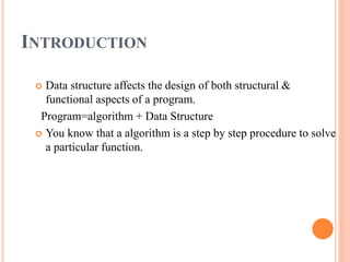
This document discusses data structures and algorithm efficiency. It defines data structures as representations of logical relationships between data elements. Data structures are classified as primitive (basic types like integers) and non-primitive (derived types like lists, stacks, queues, trees, graphs). The document explains various non-primitive data structures and their implementations. It also discusses measuring algorithm efficiency, including analyzing best, worst, and average cases. Asymptotic analysis using Big O notation is introduced as a machine-independent way to compare algorithm growth rates and determine asymptotic complexity classes.


![ARRAYS
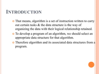
Simply, declaration of array is as follows:
int arr[10]
Where int specifies the data type or type of elements arrays
stores.
“arr” is the name of array & the number specified inside the
square brackets is the number of elements an array can store,
this is also called sized or length of array.](https://image.slidesharecdn.com/datastructuresmoduleiii-231118053822-8b9a4acf/85/data-structures-module-I-II-pptx-14-320.jpg)
![ARRAYS
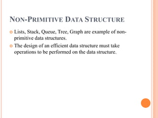
Following are some of the concepts to be remembered
about arrays:
The individual element of an array can
be accessed by specifying name of the
array, following by index or subscript
inside square brackets.
The first element of the array has index
zero[0]. It means the first element and
last element will be specified as:arr[0] &
arr[9]
Respectively.](https://image.slidesharecdn.com/datastructuresmoduleiii-231118053822-8b9a4acf/85/data-structures-module-I-II-pptx-15-320.jpg)


![ARRAYS
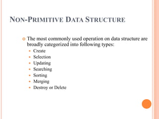
For example: Reading an array
For(i=0;i<=9;i++)
scanf(“%d”,&arr[i]);
For example: Writing an array
For(i=0;i<=9;i++)
printf(“%d”,arr[i]);](https://image.slidesharecdn.com/datastructuresmoduleiii-231118053822-8b9a4acf/85/data-structures-module-I-II-pptx-18-320.jpg)


![LISTS
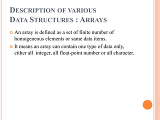
Technically each such element is referred to as a node,
therefore a list can be defined as a collection of nodes as
show bellow:
Head
AAA BBB CCC
Information field Pointer field
[Linear Liked List]](https://image.slidesharecdn.com/datastructuresmoduleiii-231118053822-8b9a4acf/85/data-structures-module-I-II-pptx-22-320.jpg)


![STACK
Insertion of element into stack is called PUSH and
deletion of element from stack is called POP.
The bellow show figure how the operations take place on
a stack:
PUSH POP
[STACK]](https://image.slidesharecdn.com/datastructuresmoduleiii-231118053822-8b9a4acf/85/data-structures-module-I-II-pptx-26-320.jpg)


![GRAPH
Example of graph:
v2
v1
v4
v5
v3
10
15
8
6
11
9
v4
v1
v2
v4
v3
[a] Directed &
Weighted Graph
[b] Undirected Graph](https://image.slidesharecdn.com/datastructuresmoduleiii-231118053822-8b9a4acf/85/data-structures-module-I-II-pptx-36-320.jpg)


![Running Time Examples (cont.’d)
Algorithm 1 Cost
arr[0] = 0; c1
arr[1] = 0; c1
arr[2] = 0; c1
...
arr[N-1] = 0; c1
-----------
c1+c1+...+c1 = c1 x N
Algorithm 2 Cost
for(i=0; i<N; i++) c2
arr[i] = 0; c1
-----------
(N+1) x c2 + N x c1 = (c2 + c1) x N + c2](https://image.slidesharecdn.com/datastructuresmoduleiii-231118053822-8b9a4acf/85/data-structures-module-I-II-pptx-86-320.jpg)
![Cost
sum = 0; c1
for(i=0; i<N; i++) c2
for(j=0; j<N; j++) c2
sum += arr[i][j]; c3
------------
c1 + c2 x (N+1) + c2 x N x (N+1) + c3 x N x N
87
Running Time Examples (cont.’d)](https://image.slidesharecdn.com/datastructuresmoduleiii-231118053822-8b9a4acf/85/data-structures-module-I-II-pptx-87-320.jpg)
![Complexity Examples
What does the following algorithm compute?
int who_knows(int a[n]) {
int m = 0;
for {int i = 0; i<n; i++}
for {int j = i+1; j<n; j++}
if ( abs(a[i] – a[j]) > m )
m = abs(a[i] – a[j]);
return m;
}
returns the maximum difference between any two
numbers in the input array
Comparisons: n-1 + n-2 + n-3 + … + 1 = (n-1)n/2 = 0.5n2 - 0.5n
Time complexity is O(n2)](https://image.slidesharecdn.com/datastructuresmoduleiii-231118053822-8b9a4acf/85/data-structures-module-I-II-pptx-88-320.jpg)
![Complexity Examples
Another algorithm solving the same problem:
int max_diff(int a[n]) {
int min = a[0];
int max = a[0];
for {int i = 1; i<n; i++}
if ( a[i] < min )
min = a[i];
else if ( a[i] > max )
max = a[i];
return max-min;
}
Comparisons: 2n - 2
Time complexity is O(n).](https://image.slidesharecdn.com/datastructuresmoduleiii-231118053822-8b9a4acf/85/data-structures-module-I-II-pptx-89-320.jpg)
![Examples of Growth Rate
/* @return Position of largest value in "A“ */
static int largest(int[] A) {
int currlarge = 0; // Position of largest
for (int i=1; i<A.length; i++)
if (A[currlarge] < A[i])
currlarge = i; // Remember position
return currlarge; // Return largest
position
}](https://image.slidesharecdn.com/datastructuresmoduleiii-231118053822-8b9a4acf/85/data-structures-module-I-II-pptx-90-320.jpg)


![Time Complexity Examples (2)
sum = 0;
for (j=1; j<=n; j++)
for (i=1; i<=j; i++)
sum++;
for (k=0; k<n; k++)
A[k] = k;](https://image.slidesharecdn.com/datastructuresmoduleiii-231118053822-8b9a4acf/85/data-structures-module-I-II-pptx-93-320.jpg)


![Traversal Singly Linked Lists
ALGORITHM FOR TRAVERSING A LINKED LIST
Step 1: [INITIALIZE] SET PTR = START
Step 2: Repeat Steps 3 and 4 while PTR != NULL
Step 3: Apply Process to PTR->DATA
Step 4: SET PTR = PTR->NEXT
[END OF LOOP]
Step 5: EXIT
void display(struct node *ptr) {
while(ptr != NULL) {
printf("%d ", ptr->data); // process
ptr = ptr->next;
}
}
Call as display(START);](https://image.slidesharecdn.com/datastructuresmoduleiii-231118053822-8b9a4acf/85/data-structures-module-I-II-pptx-108-320.jpg)

![Searching a Linked List
ALGORITHM TO SEARCH A LINKED LIST
Step 1: [INITIALIZE] SET PTR = START
Step 2: Repeat Step 3 while PTR != NULL
Step 3: IF VAL = PTR->DATA
SET POS = PTR
Go To Step 5
ELSE
SET PTR = PTR->NEXT
[END OF IF]
[END OF LOOP]
Step 4: SET POS = NULL // not found
Step 5: EXIT // found, output POS
struct node* search(struct node *ptr, int num) {
while((ptr != NULL) && (ptr->data != num)) {
ptr = ptr->next;
}
return ptr;
}
// call example, search(START, 4)](https://image.slidesharecdn.com/datastructuresmoduleiii-231118053822-8b9a4acf/85/data-structures-module-I-II-pptx-110-320.jpg)
![Inserting a Node at the Beginning
1 7 3 4 2 6 5 X
START
START
9 1 7 3 4 2 6 5 X
ALGORITHM: INSERT A NEW NODE IN THE BEGINNING OF THE LINKED LIST
Step 1: IF AVAIL = NULL, then
Write OVERFLOW
Go to Step 7
[END OF IF]
Step 2: SET New_Node = AVAIL
Step 3: SET AVAIL = AVAIL->NEXT
Step 4: SET New_Node->DATA = VAL
Step 5: SET New_Node->Next = START
Step 6: SET START = New_Node
Step 7: EXIT
See example](https://image.slidesharecdn.com/datastructuresmoduleiii-231118053822-8b9a4acf/85/data-structures-module-I-II-pptx-111-320.jpg)
![Inserting a Node at the End
1 7 3 4 2 6 5 X
START, PTR
1 7 3 4 2 6 5 9 X
START
ALGORITHM TO INSERT A NEW NODE AT THE END OF THE LINKED LIST
Step 1: IF AVAIL = NULL, then
Write OVERFLOW
Go to Step 10
[END OF IF]
Step 2: SET New_Node = AVAIL
Step 3: SET AVAIL = AVAIL->NEXT
Step 4: SET New_Node->DATA = VAL
Step 5: SET New_Node->Next = NULL
Step 6: SET PTR = START
Step 7: Repeat Step 8 while PTR->NEXT != NULL
Step 8: SET PTR = PTR ->NEXT
[END OF LOOP]
Step 9: SET PTR->NEXT = New_Node
Step 10: EXIT](https://image.slidesharecdn.com/datastructuresmoduleiii-231118053822-8b9a4acf/85/data-structures-module-I-II-pptx-112-320.jpg)
![Inserting a Node after Node that ahs Value NUM
ALGORITHM TO INSERT A NEW NODE AFTER A NODE THAT HAS VALUE
NUM
Step 1: IF AVAIL = NULL, then
Write OVERFLOW
Go to Step 12
[END OF IF]
Step 2: SET New_Node = AVAIL
Step 3: SET AVAIL = AVAIL->NEXT
Step 4: SET New_Node->DATA = VAL
Step 5: SET PTR = START
Step 6: SET PREPTR = PTR
Step 7: Repeat Steps 8 and 9 while PREPTR->DATA != NUM
Step 8: SET PREPTR = PTR
Step 9: SET PTR = PTR->NEXT
[END OF LOOP]
Step 10: PREPTR->NEXT = New_Node
Step 11: SET New_Node->NEXT = PTR
Step 12: EXIT](https://image.slidesharecdn.com/datastructuresmoduleiii-231118053822-8b9a4acf/85/data-structures-module-I-II-pptx-113-320.jpg)
![Deleting the First Node
1 7 3 4 2 6 5 X
7 3 4 2 6 5 X
START
START
Algorithm to delete the first node from the linked
list
Step 1: IF START = NULL, then
Write UNDERFLOW
Go to Step 5
[END OF IF]
Step 2: SET PTR = START
Step 3: SET START = START->NEXT
Step 4: FREE PTR
Step 5: EXIT](https://image.slidesharecdn.com/datastructuresmoduleiii-231118053822-8b9a4acf/85/data-structures-module-I-II-pptx-114-320.jpg)
![Deleting the Last Node
1 7 3 4 2 6 5 X
START, PREPTR, PTR
1 7 3 4 2 6 X 5 X
PREPTR PTR
START
ALGORITHM TO DELETE THE LAST NODE OF THE LINKED LIST
Step 1: IF START = NULL, then
Write UNDERFLOW
Go to Step 8
[END OF IF]
Step 2: SET PTR = START
Step 3: Repeat Steps 4 and 5 while PTR->NEXT != NULL
Step 4: SET PREPTR = PTR
Step 5: SET PTR = PTR->NEXT
[END OF LOOP]
Step 6: SET PREPTR->NEXT = NULL
Step 7: FREE PTR
Step 8: EXIT](https://image.slidesharecdn.com/datastructuresmoduleiii-231118053822-8b9a4acf/85/data-structures-module-I-II-pptx-115-320.jpg)

![Deleting the Node After a Given Node
ALGORITHM TO DELETE THE NODE AFTER A GIVEN NODE FROM THE
LINKED LIST
Step 1: IF START = NULL, then
Write UNDERFLOW
Go to Step 10
[END OF IF]
Step 2: SET PTR = START
Step 3: SET PREPTR = PTR
Step 4: Repeat Step 5 and 6 while PRETR->DATA != NUM
Step 5: SET PREPTR = PTR
Step 6: SET PTR = PTR->NEXT
[END OF LOOP]
Step7: SET TEMP = PTR->NEXT
Step 8: SET PREPTR->NEXT = TEMP->NEXT
Step 9: FREE TEMP
Step 10: EXIT](https://image.slidesharecdn.com/datastructuresmoduleiii-231118053822-8b9a4acf/85/data-structures-module-I-II-pptx-117-320.jpg)

![Circular Linked List
Algorithm to insert a new node in the beginning of
circular the linked list
Step 1: IF AVAIL = NULL, then
Write OVERFLOW
Go to Step 7
[END OF IF]
Step 2: SET New_Node = AVAIL
Step 3: SET AVAIL = AVAIL->NEXT
Step 4: SET New_Node->DATA = VAL
Step 5: SET PTR = START
Step 6: Repeat Step 7 while PTR->NEXT != START
Step 7: PTR = PTR->NEXT
Step 8: SET New_Node->Next = START
Step 8: SET PTR->NEXT = New_Node
Step 6: SET START = New_Node
Step 7: EXIT](https://image.slidesharecdn.com/datastructuresmoduleiii-231118053822-8b9a4acf/85/data-structures-module-I-II-pptx-119-320.jpg)

![Circular Linked List
Algorithm to insert a new node at the end of the circular
linked list
Step 1: IF AVAIL = NULL, then
Write OVERFLOW
Go to Step 7
[END OF IF]
Step 2: SET New_Node = AVAIL
Step 3: SET AVAIL = AVAIL->NEXT
Step 4: SET New_Node->DATA = VAL
Step 5: SET New_Node->Next = START
Step 6: SET PTR = START
Step 7: Repeat Step 8 while PTR->NEXT != START
Step 8: SET PTR = PTR ->NEXT
[END OF LOOP]
Step 9: SET PTR ->NEXT = New_Node
Step 10: EXIT](https://image.slidesharecdn.com/datastructuresmoduleiii-231118053822-8b9a4acf/85/data-structures-module-I-II-pptx-121-320.jpg)

![Circular Linked List
Algorithm to insert a new node after a node that has
value NUM
Step 1: IF AVAIL = NULL, then
Write OVERFLOW
Go to Step 12
[END OF IF]
Step 2: SET New_Node = AVAIL
Step 3: SET AVAIL = AVAIL->NEXT
Step 4: SET New_Node->DATA = VAL
Step 5: SET PTR = START
Step 6: SET PREPTR = PTR
Step 7: Repeat Step 8 and 9 while PTR->DATA != NUM
Step 8: SET PREPTR = PTR
Step 9: SET PTR = PTR->NEXT
[END OF LOOP]
Step 10: PREPTR->NEXT = New_Node
Step 11: SET New_Node->NEXT = PTR
Step 12: EXIT](https://image.slidesharecdn.com/datastructuresmoduleiii-231118053822-8b9a4acf/85/data-structures-module-I-II-pptx-123-320.jpg)
![Circular Linked List
Algorithm to delete the first node from the circular linked list
Step 1: IF START = NULL, then
Write UNDERFLOW
Go to Step 8
[END OF IF]
Step 2: SET PTR = START
Step 3: Repeat Step 4 while PTR->NEXT != START
Step 4: SET PTR = PTR->NEXT
[END OF IF]
Step 5: SET PTR->NEXT = START->NEXT
Step 6: FREE START
Step 7: SET START = PTR->NEXT
Step 8: EXIT](https://image.slidesharecdn.com/datastructuresmoduleiii-231118053822-8b9a4acf/85/data-structures-module-I-II-pptx-124-320.jpg)

![Circular Linked List
Algorithm to delete the last node of the circular linked
list
Step 1: IF START = NULL, then
Write UNDERFLOW
Go to Step 8
[END OF IF]
Step 2: SET PTR = START
Step 3: Repeat Step 4 while PTR->NEXT != START
Step 4: SET PREPTR = PTR
Step 5: SET PTR = PTR->NEXT
[END OF LOOP]
Step 6: SET PREPTR->NEXT = START
Step 7: FREE PTR
Step 8: EXIT](https://image.slidesharecdn.com/datastructuresmoduleiii-231118053822-8b9a4acf/85/data-structures-module-I-II-pptx-126-320.jpg)

![Circular Linked List
Algorithm to delete the node after a given node from the circular linked list
Step 1: IF START = NULL, then
Write UNDERFLOW
Go to Step 9
[END OF IF]
Step 2: SET PTR = START
Step 3: SET PREPTR = PTR
Step 4: Repeat Step 5 and 6 while PREPTR->DATA != NUM
Step 5: SET PREPTR = PTR
Step 6: SET PTR = PTR->NEXT
[END OF LOOP]
Step 7: SET PREPTR->NEXT = PTR->NEXT
Step 8: FREE PTR
Step 9: EXIT](https://image.slidesharecdn.com/datastructuresmoduleiii-231118053822-8b9a4acf/85/data-structures-module-I-II-pptx-128-320.jpg)


![Doubly Linked List
1 7 3 4 2 X
X
9 1 7 3 4
X 2 X
START
START
Algorithm to insert a new node in the beginning of the
doubly linked list
Step 1: IF AVAIL = NULL, then
Write OVERFLOW
Go to Step 8
[END OF IF]
Step 2: SET New_Node = AVAIL
Step 3: SET AVAIL = AVAIL->NEXT
Step 4: SET New_Node->DATA = VAL
Step 5: SET New_Node->PREV = NULL
Step 6: SET New_Node->Next = START
Step 7: SET START = New_Node
Step 8: EXIT](https://image.slidesharecdn.com/datastructuresmoduleiii-231118053822-8b9a4acf/85/data-structures-module-I-II-pptx-132-320.jpg)
![Doubly Linked List
1 7 3 4 2 X
X
START, PTR
1 7 3 4 2
X 9 X
PTR
Algorithm to insert a new node at the end of the doubly linked list
Step 1: IF AVAIL = NULL, then
Write OVERFLOW
Go to Step 11
[END OF IF]
Step 2: SET New_Node = AVAIL
Step 3: SET AVAIL = AVAIL->NEXT
Step 4: SET New_Node->DATA = VAL
Step 5: SET New_Node->Next = NULL
Step 6: SET PTR = START
Step 7: Repeat Step 8 while PTR->NEXT != NULL
Step 8: SET PTR = PTR->NEXT
[END OF LOOP]
Step 9: SET PTR->NEXT = New_Node
Step 10: New_Node->PREV = PTR
Step 11: EXIT](https://image.slidesharecdn.com/datastructuresmoduleiii-231118053822-8b9a4acf/85/data-structures-module-I-II-pptx-133-320.jpg)
![Doubly Linked List
Algorithm to insert a new node after a node that has
value NUM
Step 1: IF AVAIL = NULL, then
Write OVERFLOW
Go to Step 11
[END OF IF]
Step 2: SET New_Node = AVAIL
Step 3: SET AVAIL = AVAIL->NEXT
Step 4: SET New_Node->DATA = VAL
Step 5: SET PTR = START
Step 6: Repeat Step 8 while PTR->DATA != NUM
Step 7: SET PTR = PTR->NEXT
[END OF LOOP]
Step 8: New_Node->NEXT = PTR->NEXT
Step 9: SET New_Node->PREV = PTR
Step 10: SET PTR->NEXT = New_Node
Step 11: EXIT](https://image.slidesharecdn.com/datastructuresmoduleiii-231118053822-8b9a4acf/85/data-structures-module-I-II-pptx-134-320.jpg)

![Doubly Linked List
1 7 3 4 2 X
X
START, PTR
7 3 4 2 X
Algorithm to delete the first node from the doubly linked
list
Step 1: IF START = NULL, then
Write UNDERFLOW
Go to Step 6
[END OF IF]
Step 2: SET PTR = START
Step 3: SET START = START->NEXT
Step 4: SET START->PREV = NULL
Step 5: FREE PTR
Step 6: EXIT](https://image.slidesharecdn.com/datastructuresmoduleiii-231118053822-8b9a4acf/85/data-structures-module-I-II-pptx-136-320.jpg)
![Doubly Linked List
1 3 5 7 8
X 9
1
X
START, PTR
1 3 5 7 8
X 9
1
X
START PTR
1 3 5 7 8 X
X
START
Algorithm to delete the last node of the doubly linked list
Step 1: IF START = NULL, then
Write UNDERFLOW
Go to Step 7
[END OF IF]
Step 2: SET PTR = START
Step 3: Repeat Step 4 and 5 while PTR->NEXT != NULL
Step 4: SET PTR = PTR->NEXT
[END OF LOOP]
Step 5: SET PTR->PREV->NEXT = NULL
Step 6: FREE PTR
Step 7: EXIT](https://image.slidesharecdn.com/datastructuresmoduleiii-231118053822-8b9a4acf/85/data-structures-module-I-II-pptx-137-320.jpg)
![Doubly Linked List
Algorithm to delete the node after a given node from the
doubly linked list
Step 1: IF START = NULL, then
Write UNDERFLOW
Go to Step 9
[END OF IF]
Step 2: SET PTR = START
Step 3: Repeat Step 4 while PTR->DATA != NUM
Step 4: SET PTR = PTR->NEXT
[END OF LOOP]
Step 5: SET TEMP = PTR->NEXT
Step 6: SET PTR->NEXT = TEMP->NEXT
Step 7: SET TEMP->NEXT->PREV = PTR
Step 8: FREE TEMP
Step 9: EXIT](https://image.slidesharecdn.com/datastructuresmoduleiii-231118053822-8b9a4acf/85/data-structures-module-I-II-pptx-138-320.jpg)


![Circular Queue
Bellow show a figure a empty circular queue Q[5]
which can accommodate five elements.
`
Q[0] Q[1]
Q[2]
Q[3]
Q[4]
Fig: Circular Queue](https://image.slidesharecdn.com/datastructuresmoduleiii-231118053822-8b9a4acf/85/data-structures-module-I-II-pptx-149-320.jpg)

![Double Ended Queue (Deque)
There are:
Input-restricted Deque.
Output-restricted Deque.
Bellow show a figure a empty Deque Q[5] which
can accommodate five elements.
Q[0] Q[1] Q[2] Q[3] Q[4]
deletion
deletion
insertion
insertion
Fig: A Deque](https://image.slidesharecdn.com/datastructuresmoduleiii-231118053822-8b9a4acf/85/data-structures-module-I-II-pptx-151-320.jpg)
![Double Ended Queue (Deque)
There are:
Input-restricted Deque: An input restricted
Deque restricts the insertion of the elements at
one end only, the deletion of elements can be
done at both the end of a queue.
10 20 30 40 50
Q[0] Q[1] Q[2] Q[3] Q[4]
deletion
deletion
insertion
Fig: A representation of an input-restricted Deque
F R](https://image.slidesharecdn.com/datastructuresmoduleiii-231118053822-8b9a4acf/85/data-structures-module-I-II-pptx-152-320.jpg)
![Double Ended Queue (Deque)
There are:
Output-restricted Deque: on the contrary, an
Output-restricted Deque, restricts the deletion of
elements at one end only, and allows insertion to
be done at both the ends of a Deque.
10 20 30 40 50
Q[0] Q[1] Q[2] Q[3] Q[4]
insertion
deletion
insertion
Fig: A representation of an Output-restricted Deque
F R](https://image.slidesharecdn.com/datastructuresmoduleiii-231118053822-8b9a4acf/85/data-structures-module-I-II-pptx-153-320.jpg)


![169
Two Stacks in a Single Array –
Solution Details (continued)
S1.PUSH (val)
if (t1 > t2)
error "stack overflow"
A[t1] = val
t1++
S2.PUSH (val)
if (t1 > t2)
error "stack overflow"
A[t2] = val
t2--](https://image.slidesharecdn.com/datastructuresmoduleiii-231118053822-8b9a4acf/85/data-structures-module-I-II-pptx-169-320.jpg)
![170
Two Stacks in a Single Array –
Solution Details (continued)
S1.POP
if (t1 = 0)
error "stack underflow"
t1--
return A[t1]
S2.POP
if (t2 = n - 1)
error "stack underflow"
t2++
return A[t2]](https://image.slidesharecdn.com/datastructuresmoduleiii-231118053822-8b9a4acf/85/data-structures-module-I-II-pptx-170-320.jpg)
![171
Two Stacks in a Single Array –
Solution Details (continued)
S1.TOP
if (t1 = 0)
error "stack is empty"
return A[t1]
S2.TOP
if (t2 = n - 1)
error "stack is empty"
return A[t2]](https://image.slidesharecdn.com/datastructuresmoduleiii-231118053822-8b9a4acf/85/data-structures-module-I-II-pptx-171-320.jpg)