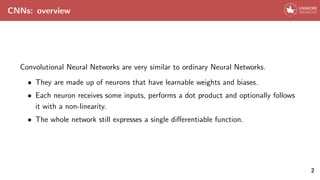
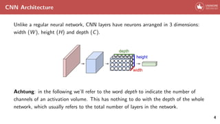
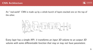
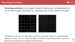
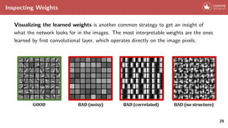
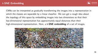
The document provides an overview of Convolutional Neural Networks (CNNs), detailing their architecture, core components such as convolutional and pooling layers, and activation functions. It discusses the significance of CNNs in image processing, their efficiency compared to traditional neural networks, and introduces the VGG network case study as an example of a successful CNN architecture. Additionally, the document addresses concepts like transfer learning and the interpretability of CNNs, highlighting challenges and common practices in the field.

1. Deep Learning and Temporal Data Processing
2 - Convolutional Neural Networks
Andrea Palazzi
December 20, 2017
University of Modena and Reggio Emilia

2. Agenda
Introduction
Architecture
Case Study: VGG Network
Visualizing what CNNs Learn
Transfer Learning
Credits
References
1

3. Introduction

4. CNNs: overview
Convolutional Neural Networks are very similar to ordinary Neural Networks.
• They are made up of neurons that have learnable weights and biases.
• Each neuron receives some inputs, performs a dot product and optionally follows
it with a non-linearity.
• The whole network still expresses a single differentiable function.
2

5. CNNs: overview
However, CNNs make the explicit assumption that inputs are images.
• This architecture constraint paves the way to more efficient implementation,
better performance and a vastly reduced amount of learnable parameters
w.r.t. fully-connected deep networks.
Most important peculiarities of CNNs are presented in the following slides.
3

6. Architecture

7. CNN Architecture
Unlike a regular neural network, CNN layers have neurons arranged in 3 dimensions:
width (W ), height (H) and depth (C).
Achtung: in the following we’ll refer to the word depth to indicate the number of
channels of an activation volume. This has nothing to do with the depth of the whole
network, which usually refers to the total number of layers in the network.
4

8. CNN Architecture
An ”real-world” CNN is made up by a whole bunch of layers stacked one on the top of
the other.
Every layer has a simple API: it transforms an input 3D volume to an output 3D
volume with some differentiable function that may or may not have parameters.
5

9. Convolutional Layers
The Convolutional Layer is the core building block of convolutional neural networks.
Intuition: every convolutional layer is equipped with a set of learnable filters. During
the forward pass, each filter is convolved with the input volume thus producing a 2D
activation map. One map for each filter is produced. The output volume is then made
up by stacking all activation maps produced one on the top of the other.
e.g. Result of N = 6 filters of kernel size K = 5x5 convolved on input image.
6

10. Convolutional Layers

11. Convolutional Layers
Each convolutional layer has three main hyperparameters:
• Number of filters N
• Kernel size K, the spatial size of the filters convolved
• Filter stride S, factor by which to downscale
The presence and amount of spatial padding P on the input volume may be considered
an additional hyperparameter. In practice padding is usually performed to avoid
headaches caused by convolutions ”eating the borders”.
7

12. Visualizing Convolution 2D
Convolution 2D, half padding, stride S = 1.
8

13. Visualizing Convolution 2D
Convolution 2D, no padding, stride S = 2.
9

14. Convolutional Layers: Local Connectivity
Looking closer, neurons in a CNN perform the very same operation of the neurons we
already know from DNN. X
i
wi xi + b
However, in convolutional layers neurons
are only locally connected to the input
volume. The small region that each
neuron ”sees” of the previous layer is
usually referred to as the receptive field
of the neuron.
10

15. Convolutional Layers: Parameter Sharing
Assumption: if a feature is useful to compute at some spatial location (x, y), then it
should be useful to compute also at different locations (xi , yi ). Thus, we constrain
the neurons in each depth slice to use the same weights and bias.
If all neurons in a single depth slice are using the same weight vector, then the forward
pass of the convolutional layer can in each depth slice be computed as a convolution of
the neuron’s weights with the input volume (hence the name). This is why it is
common to refer to each set of weights as a filter (or a kernel), that is convolved with
the input.
11

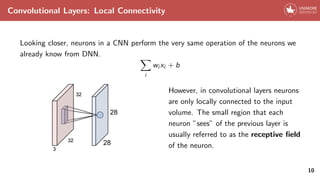
16. Convolutional Layers: Parameter Sharing
Example of weights learned by [6]. Each of the 96 filters shown here is of size [11x11x3], and
each one is shared by the 55*55 neurons in one depth slice. Notice that the parameter sharing
assumption is relatively reasonable: If detecting a horizontal edge is important at some location
in the image, it should intuitively be useful at some other location as well due to the
translationally-invariant structure of images.
12

17. Convolutional Layers: Number of Learnable Parameters
Given an input volume of size H1 x W1 x C1, the number of learnable parameters of
a convolutional layer with N filters and kernel size KxK is:
tot learnable = N ∗ K ∗ K ∗ C1 + N
Explanation: there are N filters which convolve on input volume. The neural connection is local
on width and height, but extends for the full depth of input volume, so there are K ∗ K ∗ C1
parameters for each filter. Furthermore, each filter has an additive learnable bias.
13

18. Pooling Layers

19. Pooling Layers: overview
Pooling layers spatially subsample the input volume.
Each depth slice of the input is processed independently.
Two hyperparameters:
• Pool size K, which is the size of the pooling window
• Pool stride S, which is the factor by which to downscale 14

20. Pooling Layers: types
The pooling function may be considered an additional hyperparameter.
In principle, many different functions could be used.
In practice, the max pooling is by far the most common
hn
i (x, y) = maxx̄,ȳ∈N(x,y)hn−1
i (x̄, ȳ)
Another common pooling function is the average
hn
i (x, y) =
1
K
X
x̄,ȳ∈N(x,y)
hn−1
i (x̄, ȳ)
15

21. Pooling Layers: why
Pooling layers are widely used for a number of reasons:
• Gain robustness to exact location of the features
• Reduce computational (memory) cost
• Help preventing overfitting
• Increase receptive field of following layers
Most common configuration: pool size K = 2x2, stride S = 2. In this setting 75% of
input volume activations are discarded.
16

22. Pooling Layers: why not
The loss of spatial resolution is not always beneficial.
e.g. semantic segmentation
There’s a lot of research on getting rid of pooling layers while mantaining the benefits
(e.g. [9, 11]). We’ll see if future architecture will still feature pooling layers.
17

23. Activation Layers

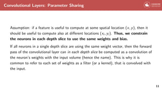
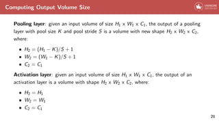
24. Activation Layers
Activation layers compute non-linear activation function elementwise on the input
volume. The most common activations are ReLu, sigmoid and tanh.
Sigmoid Tanh ReLu
Nonetheless, more complex activation functions exist [3, 2].
18

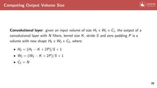
25. Activation Layers
ReLu wins
ReLu was found to greatly accelerate the convergence of SGD compared to
sigmoid/tanh functions [6]. Furthermore, ReLu can be implemented by a simple
threshold, w.r.t. other activations which require complex operations.
Why using non-linear activations at all?
Composition of linear functions is a linear function. Without nonlinearities, neural
networks would reduce to 1 layer logistic regression.
19

26. Computing Output Volume Size
Convolutional layer: given an input volume of size H1 x W1 x C1, the output of a
convolutional layer with N filters, kernel size K, stride S and zero padding P is a
volume with new shape H2 x W2 x C2, where:
• H2 = (H1 − K + 2P)/S + 1
• W2 = (W1 − K + 2P)/S + 1
• C2 = N
20

27. Computing Output Volume Size
Pooling layer: given an input volume of size H1 x W1 x C1, the output of a pooling
layer with pool size K and pool stride S is a volume with new shape H2 x W2 x C2,
where:
• H2 = (H1 − K)/S + 1
• W2 = (W1 − K)/S + 1
• C2 = C1
Activation layer: given an input volume of size H1 x W1 x C1, the output of an
activation layer is a volume with shape H2 x W2 x C2, where:
• H2 = H1
• W2 = W1
• C2 = C1
21

28. Advanced CNN Architectures
More complex CNN architectures have recently been demonstrated to perform better
than the traditional conv -> relu -> pool stack architecture.
These architectures usually feature different graph topologies and much more intricate
connectivity structures (e.g. [4, 10]).
However, these advanced architectures are out of the scope of these lectures.
22

29. Case Study: VGG Network

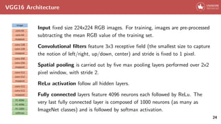
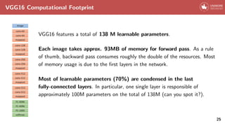
30. VGG
VGG [8] indicates a deep convolutional network for image recognition developed and
trained in 2014 by the Oxford Vision Geometry Group.
This network is well-known for a variety of reasons:
• Performance of the network is (was) great. In 2014 VGG team secured the first
and the second places in the localization and classification challenge on ImageNet;
• Pre-trained weights were released in Caffe [5] and converted by the deep
learning community in a variety of other frameworks;
• Architectural choices by the authors led to a very neat network model,
successively taken as guideline for a number of future works.
23

31. VGG16 Architecture
Input fixed size 224x224 RGB images. For training, images are pre-processed
subtracting the mean RGB value of the training set.
Convolutional filters feature 3x3 receptive field (the smallest size to capture
the notion of left/right, up/down, center) and stride is fixed to 1 pixel.
Spatial pooling is carried out by five max pooling layers performed over 2x2
pixel window, with stride 2.
ReLu activation follow all hidden layers.
Fully connected layers feature 4096 neurons each followed by ReLu. The
very last fully connected layer is composed of 1000 neurons (as many as
ImageNet classes) and is followed by softmax activation.
24

32. VGG16 Computational Footprint
VGG16 features a total of 138 M learnable parameters.
Each image takes approx. 93MB of memory for forward pass. As a rule
of thumb, backward pass consumes roughly the double of the resources. Most
of memory usage is due to the first layers in the network.
Most of learnable parameters (70%) are condensed in the last
fully-connected layers. In particular, one single layer is responsible of
approximately 100M parameters on the total of 138M (can you spot it?).
25

33. Visualizing what CNNs Learn

34. The Myth of Interpretability
Convolutional neural networks have often been criticized for their lack of
interpretability[7]. The main objection is to deal with big and complex black boxes,
that give correct results even if in which we have no cue of what’s happening inside.
26

35. The Myth of Interpretability
On the other side, linear models and decision trees are often presented as example
of ”champions” of interpretability. The debate whether a logistic regression would be
more or less interpretable than a deep network is complex out the scope of this lecture.
Partly as a response to this criticism, several methods have been developed in
literature to visualize what a CNN learned. Let’s see some examples.
27

36. Visualizing Activations
Visualizing activations of the network during the forward pass is straightforward and
can be useful to detect dead filters (i.e. activations that are zero whatever the input).
Activations on the 1st conv layer (left), and the 5th conv layer (right) of a trained AlexNet
looking at a picture of a cat. Every box shows an activation map corresponding to some filter.
Notice that the activations are sparse and mostly local.
28

37. Inspecting Weights
Visualizing the learned weights is another common strategy to get an insight of
what the network looks for in the images. The most interpretable weights are the ones
learned by first convolutional layer, which operates directly on the image pixels.
29

38. Partially Occluding the Images
To investigate which portion of the input image most contributed to a certain
prediction, we can slide an occluding object on the input, and seeing how the class
probability changes as a function of the position of the occluder object [12].
30

39. t-SNE Embedding
CNNs can be interpreted as gradually transforming the images into a representation in
which the classes are separable by a linear classifier. We can get a rough idea about
the topology of this space by embedding images into two dimensions so that their
low-dimensional representation has approximately equal distances than their
high-dimensional representation. Here, a t-SNE embedding of a set of images.
31

40. Transfer Learning

41. Transfer Learning
“You need a lot of a data
if you want to train/use CNNs”
32

42. Transfer Learning
“You need a lot of a data
if you want to train/use CNNs”
33

43. Transfer Learning
In practice, for many applications there is no need to retrain an entire CNN
from scratch.
Conversely, few ”famous” CNN architectures (e.g. VGG [8], ResNet [4]) pretrained on
ImageNet [1] are often used as initialization or feature extractor for a variety of tasks.
34

44. Transfer Learning
Overview of three different training scenarios.
35

45. Transfer Learning
Deciding which portion of the network must be retrained is a very important choice
that will heavily influence the final model performance.
Generally speaking, two main factors influence this decision:
• size of the new dataset: if the new dataset is small, fine-tune big portion of the
network is likely to lead to overfitting. The best choice might be to train a linear
classifier of CNN features.
• similarity of the new data w.r.t. the original dataset: the more similar is the
new dataset w.r.t. the old one, the more we can confidently fine-tune the model
without risking to overfit (given that we have enough data to do it).
36

46. Transfer Learning
Rule of thumb for deciding how much of the model is to be retrained. 37

47. Credits

48. Credits i
These slides heavily borrow from a number of awesome sources. I’m really grateful to
all the people who take the time to share their knowledge on this subject with others.
In particular:
• Stanford CS231n Convolutional Neural Networks for Visual Recognition
http://cs231n.stanford.edu/
• Stanford CS20SI TensorFlow for Deep Learning Research
http://web.stanford.edu/class/cs20si/syllabus.html
• Deep Learning Book (GoodFellow, Bengio, Courville)
http://www.deeplearningbook.org/
38

49. Credits ii
• Marc’Aurelio Ranzato, ”Large-Scale Visual Recognition with Deep Learning”
www.cs.toronto.edu/~ranzato/publications/ranzato_cvpr13.pdf
• Convolution arithmetic animations
https://github.com/vdumoulin/conv_arithmetic
• Andrej Karphathy personal blog
http://karpathy.github.io/
• WildML blog on AI, DL and NLP
http://www.wildml.com/
• Michael Nielsen Deep Learning online book
http://neuralnetworksanddeeplearning.com/
39

50. References

51. References i
[1] J. Deng, W. Dong, R. Socher, L.-J. Li, K. Li, and L. Fei-Fei.
Imagenet: A large-scale hierarchical image database.
In Computer Vision and Pattern Recognition, 2009. CVPR 2009. IEEE Conference
on, pages 248–255. IEEE, 2009.
[2] I. J. Goodfellow, D. Warde-Farley, M. Mirza, A. Courville, and Y. Bengio.
Maxout networks.
arXiv preprint arXiv:1302.4389, 2013.
40

52. References ii
[3] K. He, X. Zhang, S. Ren, and J. Sun.
Delving deep into rectifiers: Surpassing human-level performance on
imagenet classification.
In Proceedings of the IEEE international conference on computer vision, pages
1026–1034, 2015.
[4] K. He, X. Zhang, S. Ren, and J. Sun.
Deep residual learning for image recognition.
In Proceedings of the IEEE conference on computer vision and pattern
recognition, pages 770–778, 2016.
41

53. References iii
[5] Y. Jia, E. Shelhamer, J. Donahue, S. Karayev, J. Long, R. Girshick,
S. Guadarrama, and T. Darrell.
Caffe: Convolutional architecture for fast feature embedding.
arXiv preprint arXiv:1408.5093, 2014.
[6] A. Krizhevsky, I. Sutskever, and G. E. Hinton.
Imagenet classification with deep convolutional neural networks.
In Advances in neural information processing systems, pages 1097–1105, 2012.
[7] Z. C. Lipton.
The mythos of model interpretability.
arXiv preprint arXiv:1606.03490, 2016.
42

54. References iv
[8] K. Simonyan and A. Zisserman.
Very deep convolutional networks for large-scale image recognition.
arXiv preprint arXiv:1409.1556, 2014.
[9] J. T. Springenberg, A. Dosovitskiy, T. Brox, and M. Riedmiller.
Striving for simplicity: The all convolutional net.
arXiv preprint arXiv:1412.6806, 2014.
[10] C. Szegedy, V. Vanhoucke, S. Ioffe, J. Shlens, and Z. Wojna.
Rethinking the inception architecture for computer vision.
In Proceedings of the IEEE Conference on Computer Vision and Pattern
Recognition, pages 2818–2826, 2016.
43

55. References v
[11] F. Yu and V. Koltun.
Multi-scale context aggregation by dilated convolutions.
arXiv preprint arXiv:1511.07122, 2015.
[12] M. D. Zeiler and R. Fergus.
Visualizing and understanding convolutional networks.
In European conference on computer vision, pages 818–833. Springer, 2014.
44