This document provides an overview of multi-armed bandit algorithms from an algorithmic perspective. It introduces the multi-armed bandit problem and defines it as a reinforcement learning problem where an agent must balance exploring unknown arms versus exploiting the best known arm to maximize rewards over time. The document summarizes several common bandit algorithms, including epsilon-greedy, upper confidence bound, and Thompson sampling. It also discusses extensions for non-stationary and contextual multi-armed bandit problems.

1. MULTI-ARMED BANDIT:
AN ALGORITHMIC PERSPECTIVE
Gabriele Sottocornola
gsottocornola[at]unibz[dot]it
Free University of Bozen-Bolzano – University of Milano-Bicocca
December 13th 2021

2. Overview
1. Introduction
2. MAB Policies
a. ε-greedy
b. Upper Confidence Bound
c. Thompson Sampling
3. Non-stationary MAB
4. Contextual MAB
5. Counterfactual MAB with Unobserved Confounders

3. INTRODUCTION

4. Introduction
• From one-armed bandit (i.e., the slot machine) to multi-armed bandit
(MAB) problem (Robbins, 1952)
• If each slot has a different payoff rate, how do you efficiently learn
which is the best one, getting the most money in limited time?

5. Definition(s)
• Reinforcement Learning: At each time step t, an agent choose one
action at among n actions (i.e., arms), based on its knowledge of the
environment, and observes a reward rt
• Machine Learning: We want to learn the parameters of a set of n
probability distributions (i.e., arms), while, at each time step t,
sampling a value rt from chosen distribution at
• Each arm 𝑎! ∈ 𝐴 is associated with an (hidden) mean reward value 𝜇!
• The goal is to maximize the (expected) cumulative reward over a
number of time steps T. Alternatively minimize the regret
𝑅" = '
#$%
"
𝑟# ; *
𝑅" = '
#$%
"
E[𝑟#] ; 𝜌 = 𝑇𝜇∗
− *
𝑅"

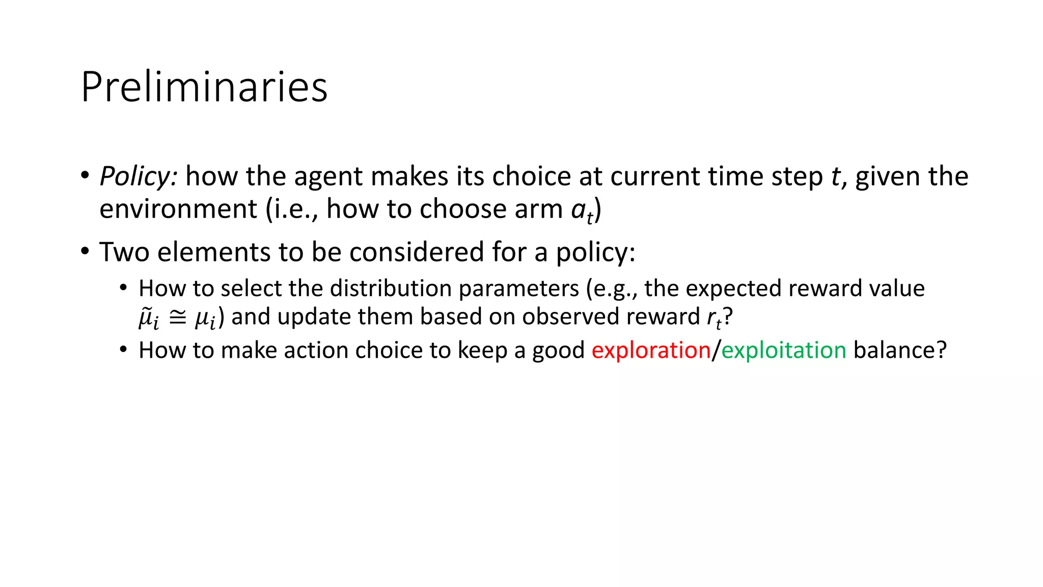
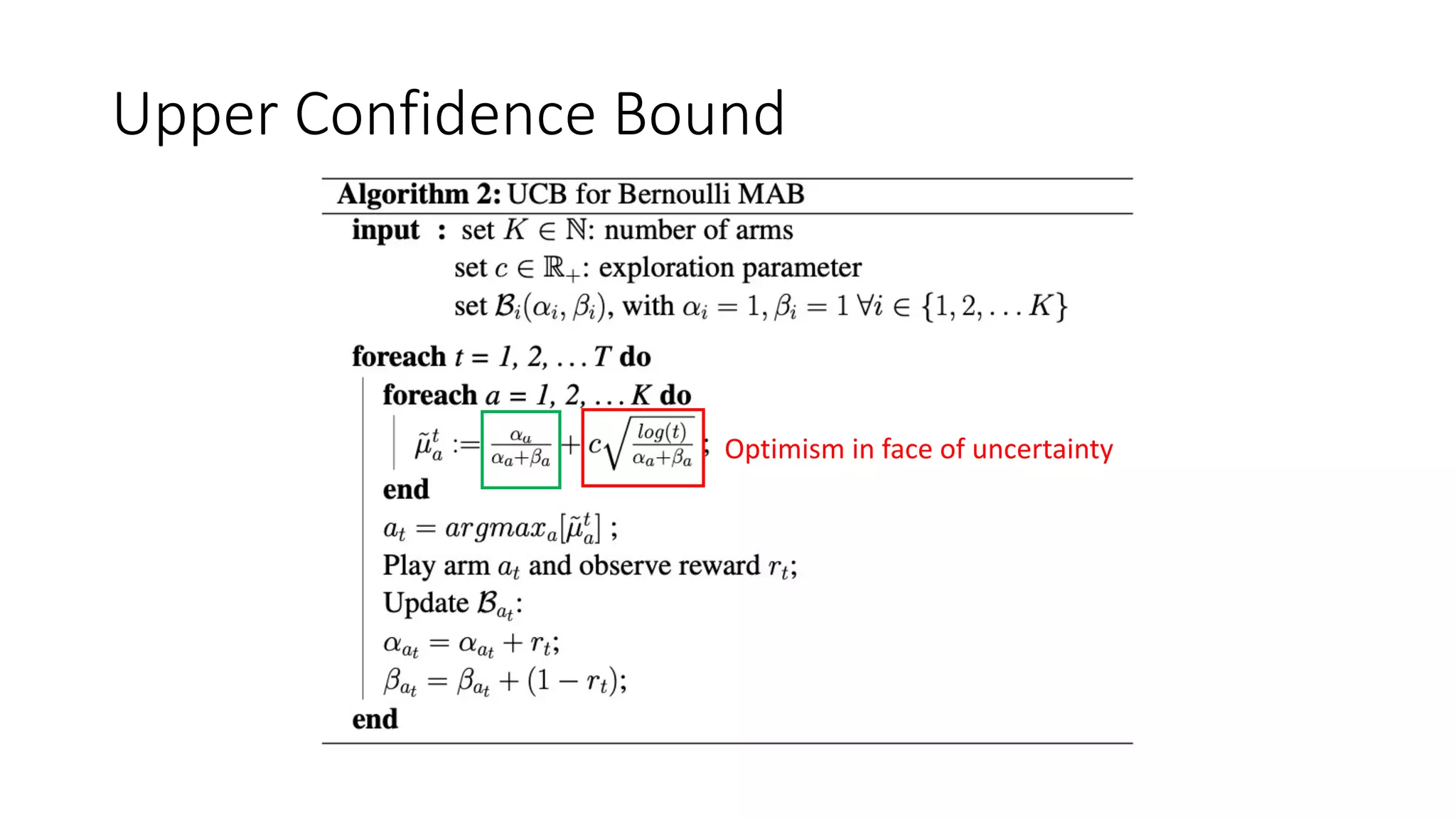
6. Preliminaries
• Exploration/exploitation decision making trade-off
• Exploration: gather information about different arms
• Exploitation: make the best choice given current information
• Bandit/Semi-bandit feedback: no full information available
• Online learning of the local optimal action
• Stochastic MAB with i.i.d. rewards (unless non-stationary or adversarial)
• Research directions:
• Proof of theoretical bounds [Auer et al., 2002]
• Application of MAB algorithms to real-world/simulated problems
• (Bayesian optimization) [Shahriari et al., 2015]
• Off-policy (counterfactual) learning/evaluation [Jeunen & Goethals, 2021]

7. Illustrative Example: A/B Test
• A company wants to advertise its product with three different
campaigns, to be tested for a time horizon of 90 days
• Each day, they display on the web one and collect the daily click-
through rate (i.e., the reward for that campaign)
• A standard A/B test (30 days per campaign) would be sub-optimal in
terms of expected clicks, hence loses potential costumers
• They adopt a bandit strategy to explore the effectiveness of all
campaigns while exploiting for the best one

8. 1
0
-1
DAY 1
CTR
𝝁𝟏
𝝁𝟐
𝝁𝟑

9. 1
0
-1
DAY 1
CTR

10. 1
0
-1
DAY 1
CTR

11. 1
0
-1
DAY 2
CTR

12. 1
0
-1
DAY 2
CTR

13. 1
0
-1
DAY 3
CTR

14. 1
0
-1
DAY 3
CTR

15. 1
0
-1
DAY 4
CTR

16. 1
0
-1
DAY 5
CTR

18. 1
0
-1
DAY 60
CTR

19. 1
0
-1
DAY 61
CTR

20. 1
0
-1
DAY 62
CTR

21. 1
0
-1
DAY 90
CTR
𝝁𝟏
𝝁𝟐
𝝁𝟑

22. Other Applications
• Clinical trials
• Dynamic resources allocation
• Web advertising placement
• Personalized news recommendation
• Financial portfolio analysis
• …

23. Supervised Learning vs MAB
• Goal: music streaming service conversion to premium membership
• Different features to promote

24. Supervised Learning vs MAB
• Rewards for all action is observed (i.e., full-information setting)
• Supervised learning should be considered!

25. Supervised Learning vs MAB
• I can promote only one feature for each user and observe the reward
• Reward only for the selected action at each time step is returned
(Bandit setup!)

26. MAB POLICIES

27. Preliminaries
• Policy: how the agent makes its choice at current time step t, given the
environment (i.e., how to choose arm at)
• Two elements to be considered for a policy:
• How to select the distribution parameters (e.g., the expected reward value
%
𝜇$ ≅ 𝜇$) and update them based on observed reward rt?
• How to make action choice to keep a good exploration/exploitation balance?

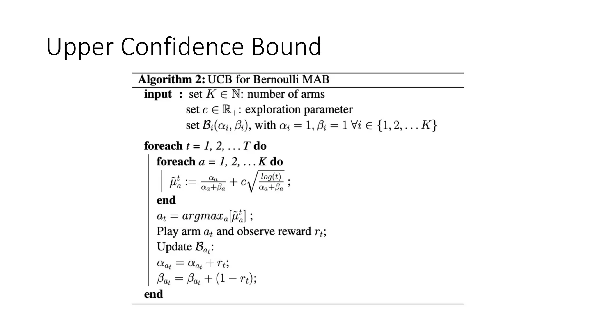
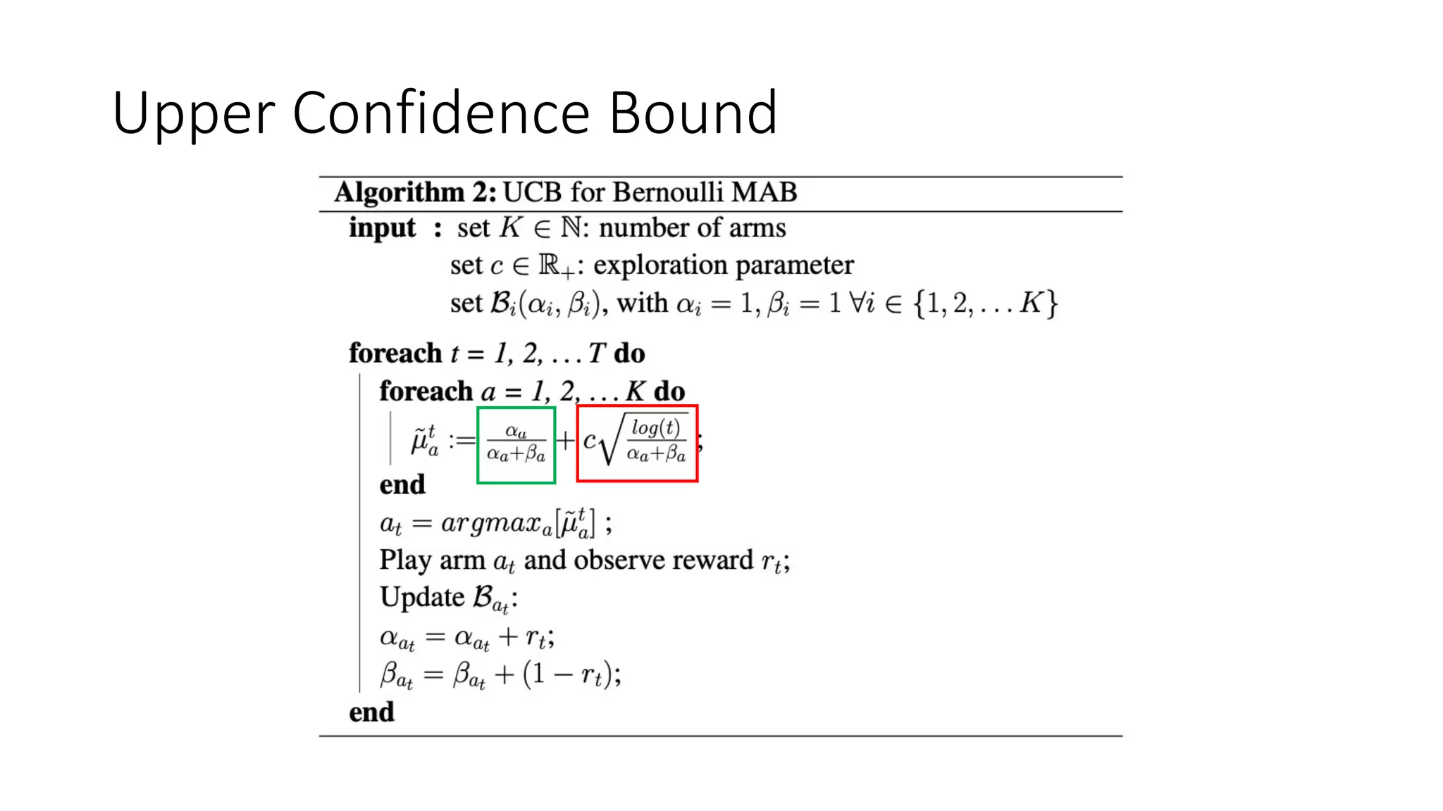
28. Preliminaries
• Assumption: Stochastic MAB with Bernoulli rewards (e.g., casino)
• Bernoulli reward 𝑟% ∈ 0, 1
• Probability of success 𝑝$ = P𝑖 𝑟% = 1 for each arm 𝑎$ ∈ 𝐴
• 𝜇$ = 𝑝$ estimated with E ℬ 𝛼, 𝛽 (i.e., Beta is Bernoulli conjugate prior, with
𝛼 successes and 𝛽 failures)
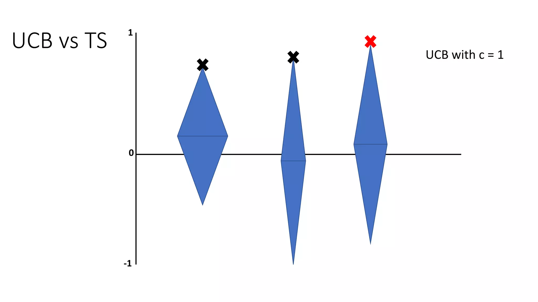
• Blueprint of a MAB action selection:
𝑎# = argmax
'
[𝑄# 𝑎 + 𝑉# 𝑎 ]

29. 𝜀-greedy

30. 𝜀-greedy

31. Beyond 𝜀-greedy
• Exploration is randomly controlled by a user-defined parameter
• Without 𝜀 is a full-exploitation (sub-optimal) algorithm
• Shortcomings:
• 𝜀 is fixed and not adaptive (solution: decaying-𝜀)
• Regret is linear in the number of round T (always same exploration rate 𝜀)
• Does not consider underlying distribution or arm-related uncertainty
• How to improve it with a policy that adapt exploration/exploitation
based on time steps t to obtain a sublinear regret?

32. Upper Confidence Bound

33. Upper Confidence Bound

34. Upper Confidence Bound
Optimism in face of uncertainty

35. https://towardsdatascience.com/the-upper-confidence-bound-ucb-bandit-algorithm-c05c2bf4c13f

36. Thompson Sampling

37. Thompson Sampling

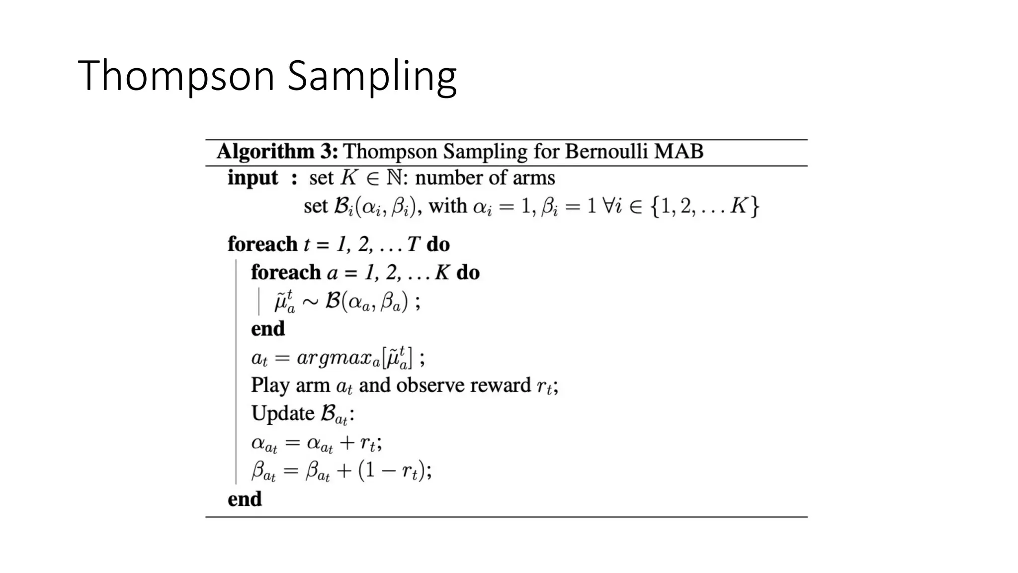
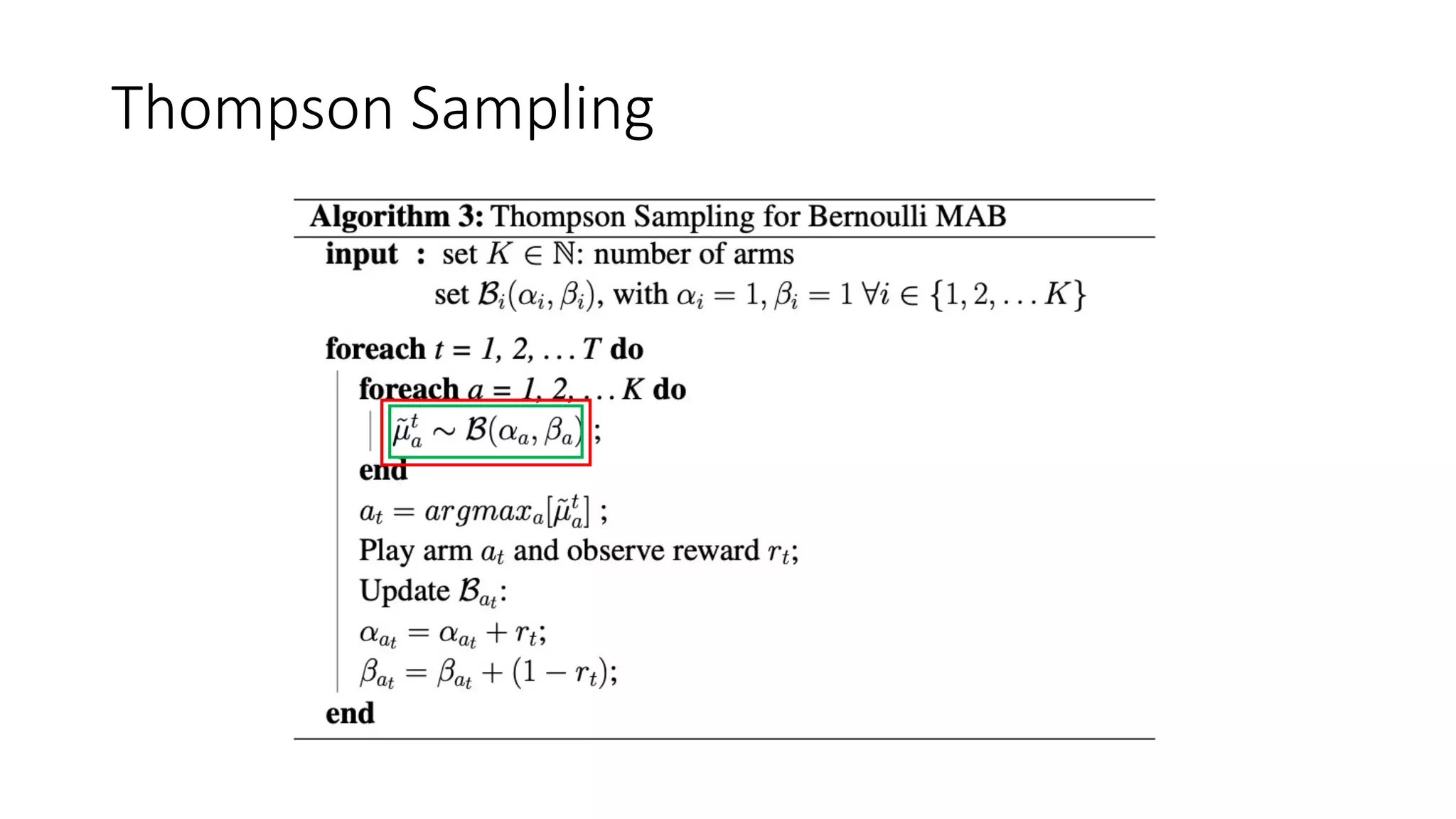
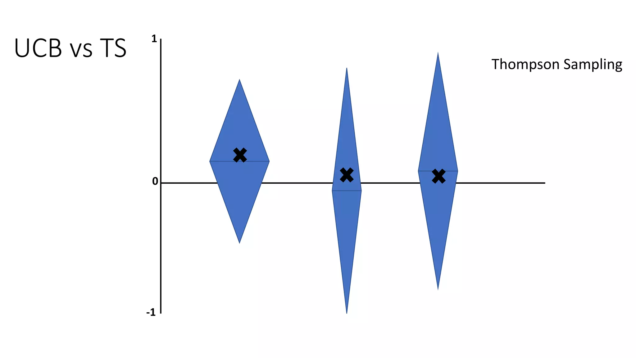
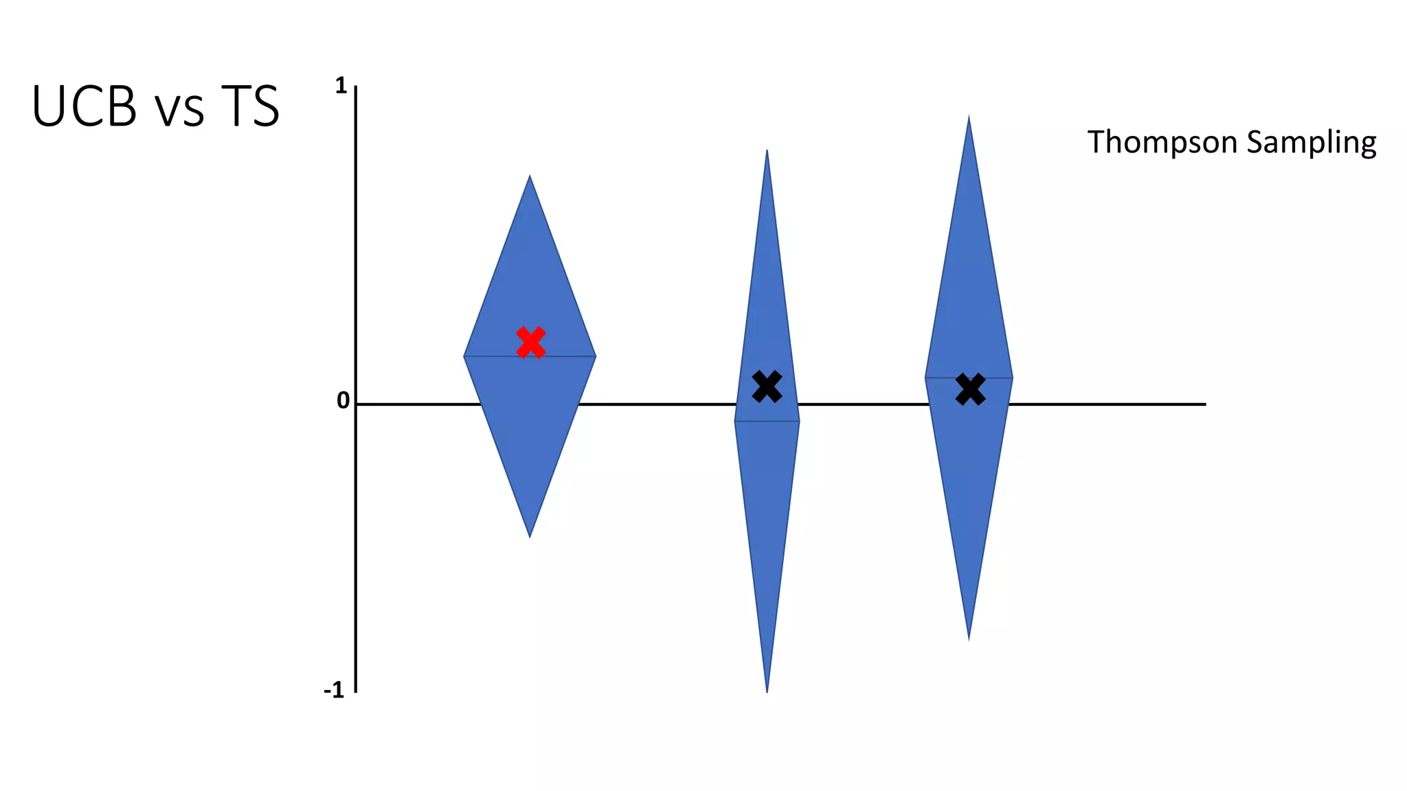
38. Thompson Sampling
Where E[ℬ] = -
𝑝! ≈ 𝑝! of Bernoulli

39. UCB vs TS
1
0
-1

40. UCB vs TS
1
0
-1
UCB with c = 1

41. UCB vs TS
1
0
-1
UCB with c = 1

42. UCB vs TS
1
0
-1
Thompson Sampling

43. UCB vs TS
1
0
-1
Thompson Sampling

44. NON-STATIONARY MAB

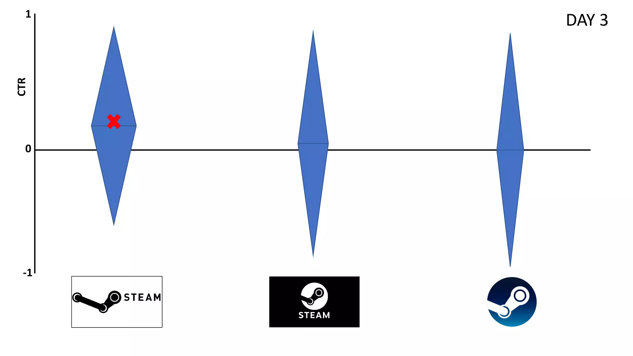
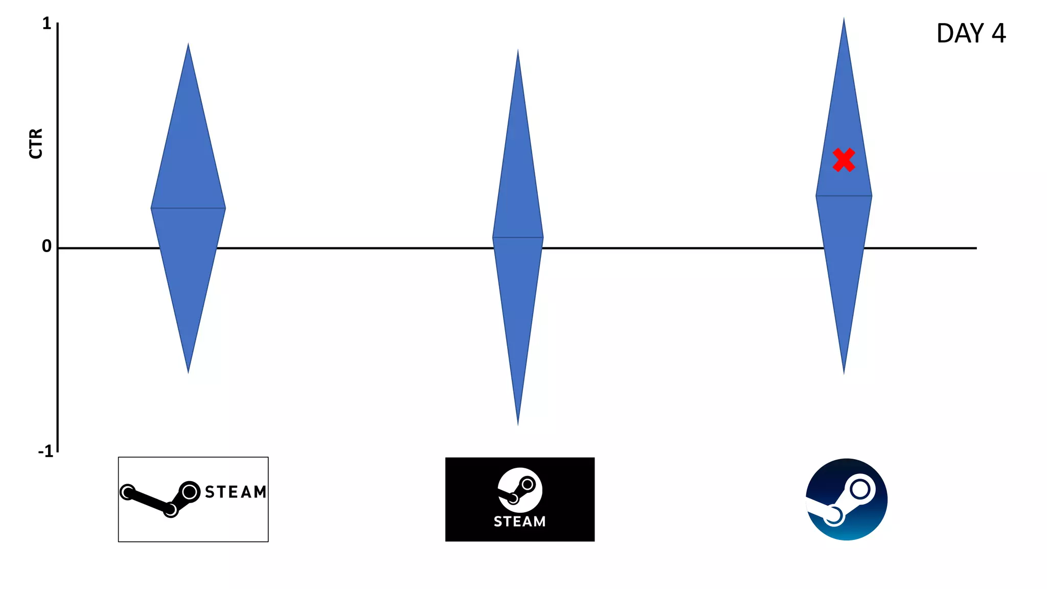
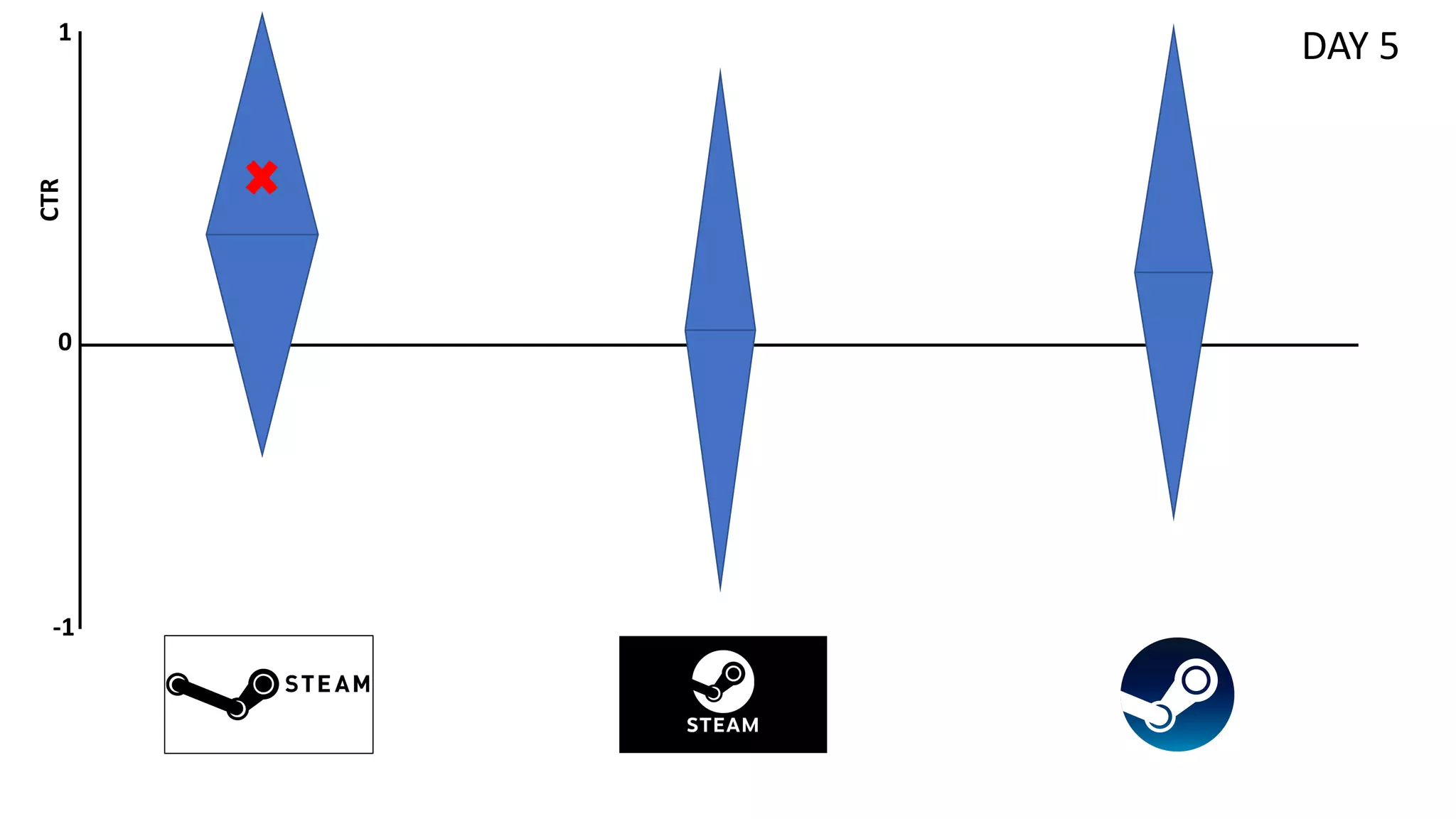
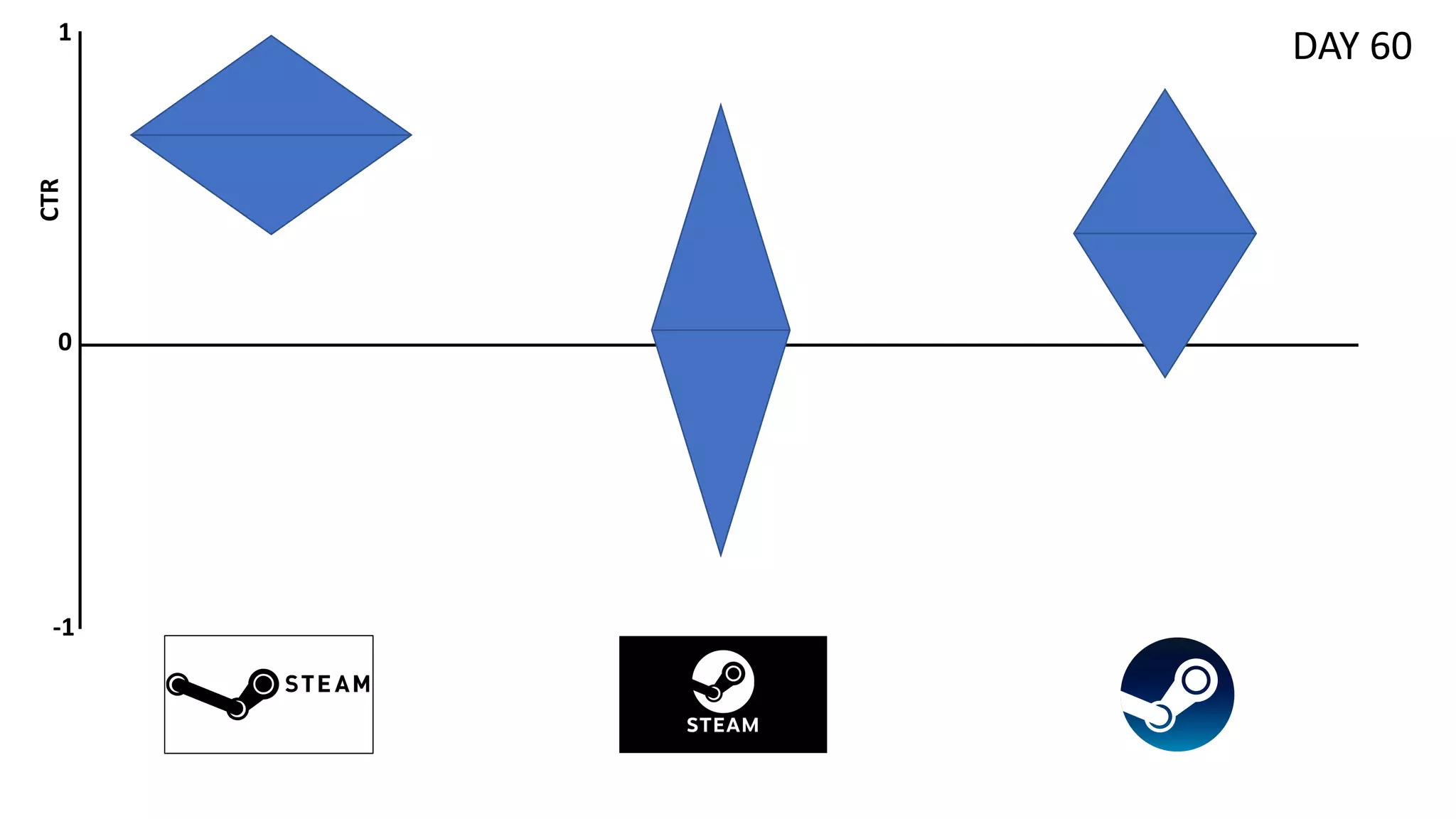
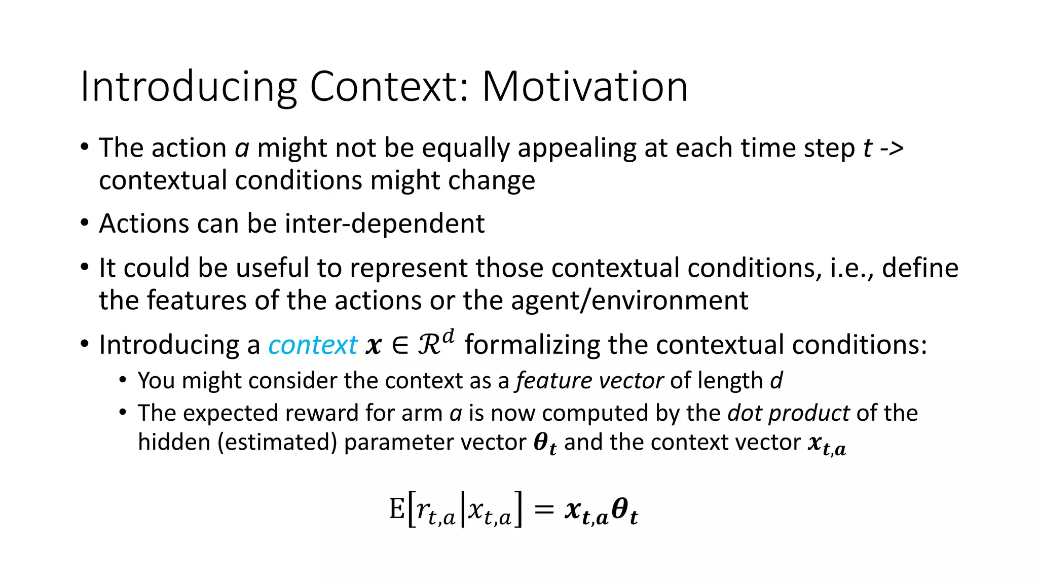
45. Motivation
• Relax the assumption of rewards being drawn i.i.d. -> Expected reward
distributions evolve over time ∃𝑡 , 𝑖 ∶ 𝜇!
#
≠ 𝜇!
#0%
• 𝑅" = ∑#$%
"
𝑟# ; *
𝑅" = ∑#$%
"
E[𝑟#] ; 𝜌 = ∑#$%
"
𝜇#,∗
− *
𝑅"
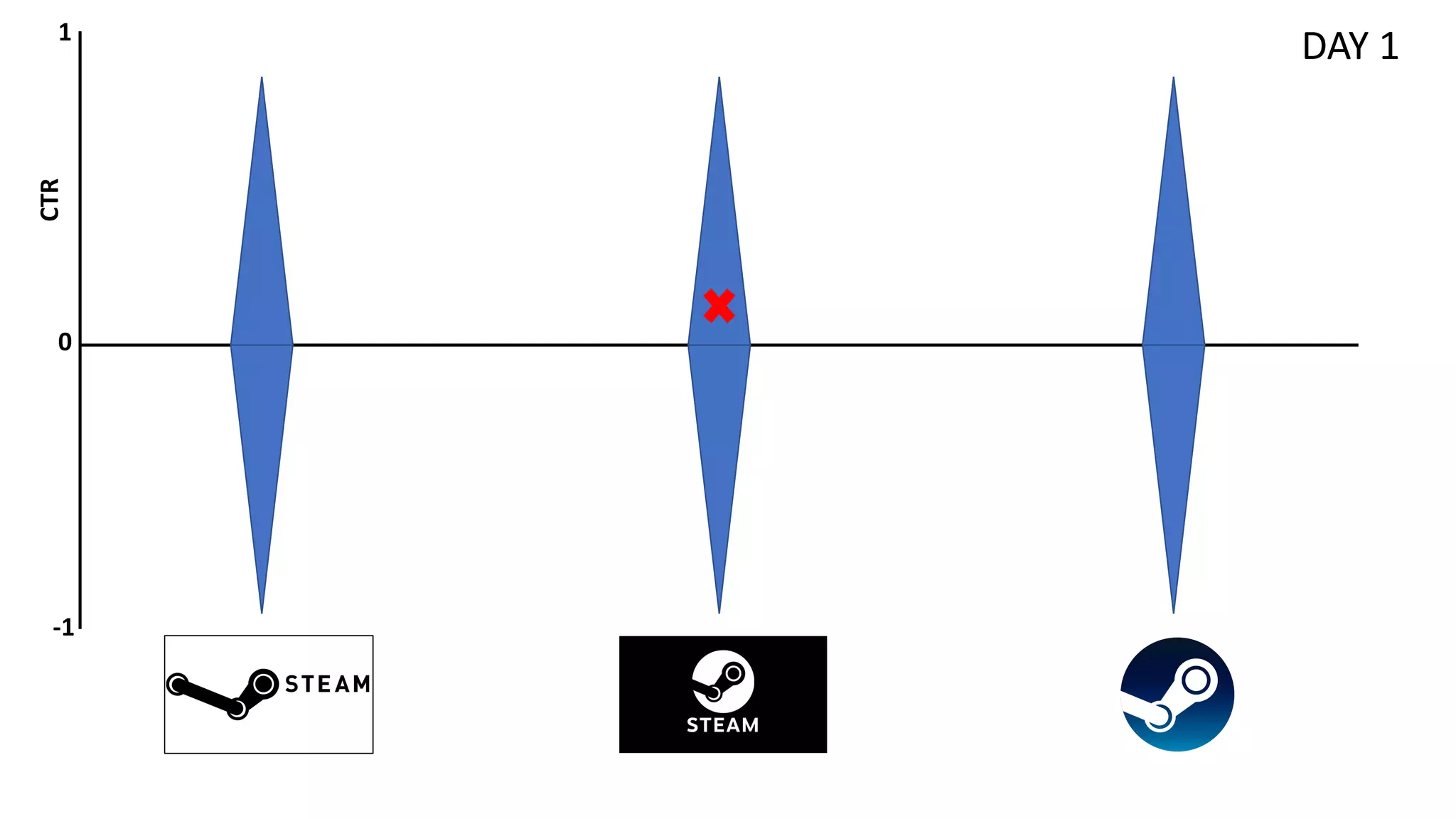
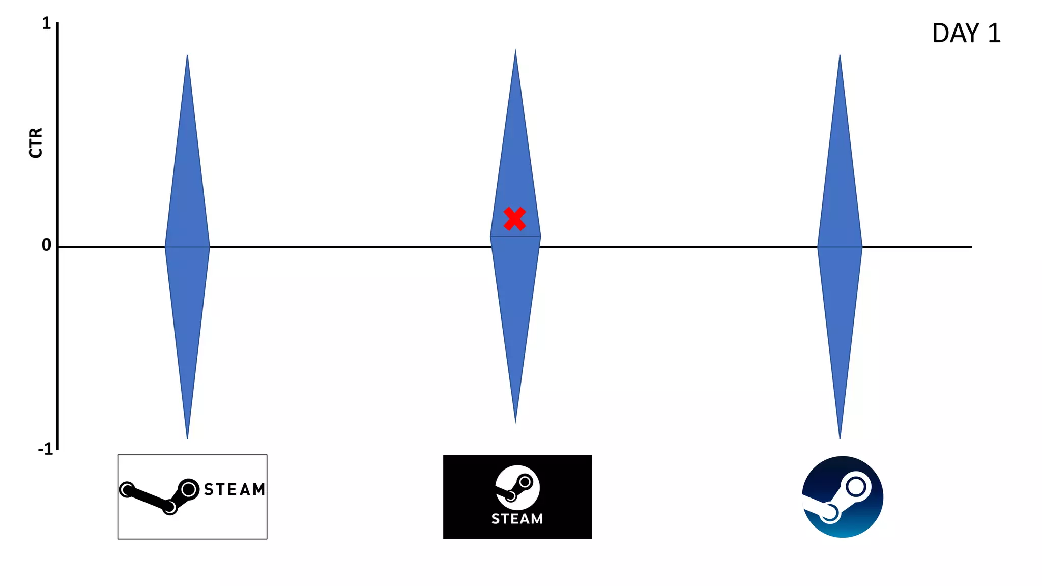
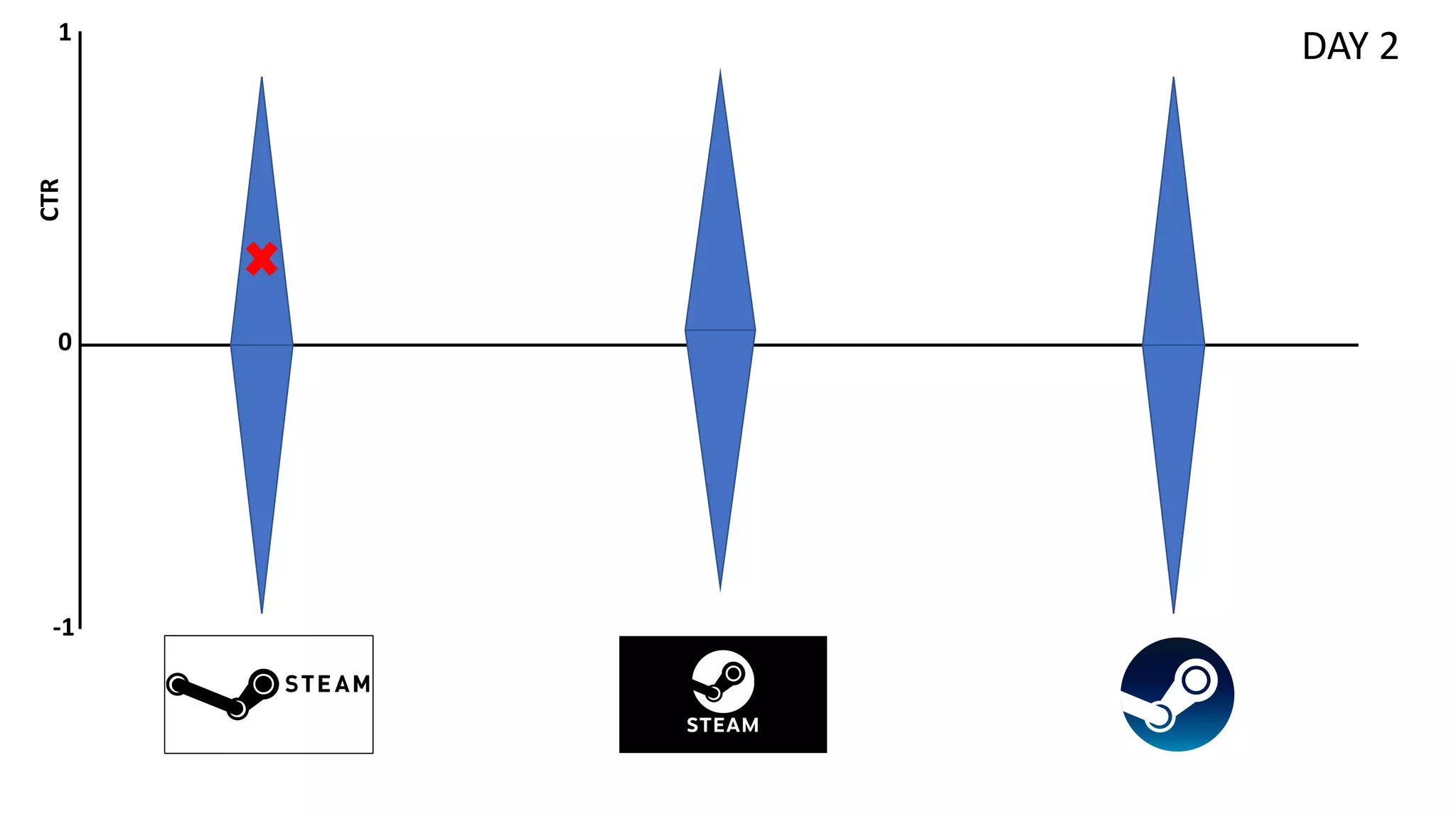
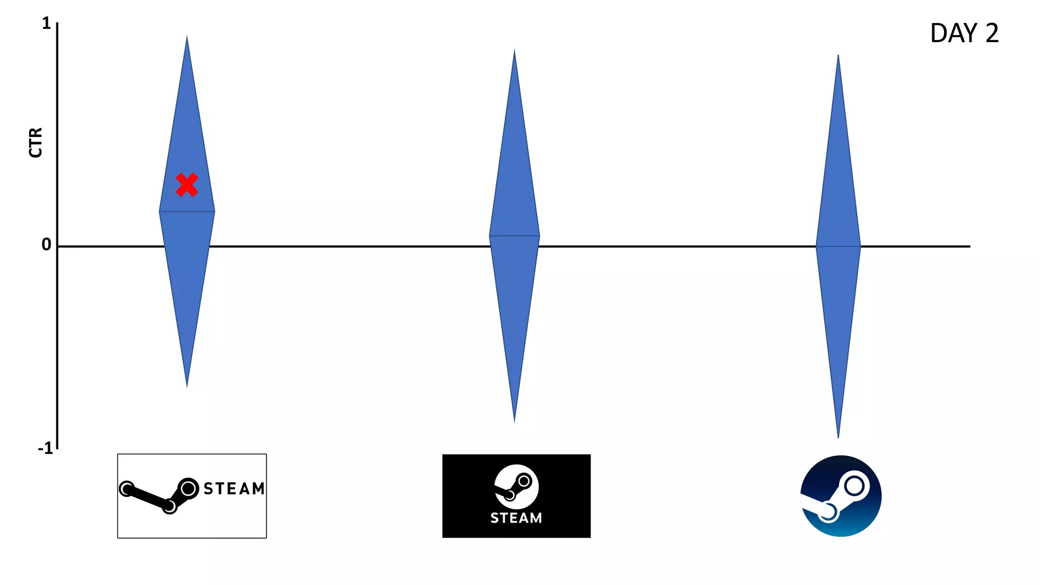
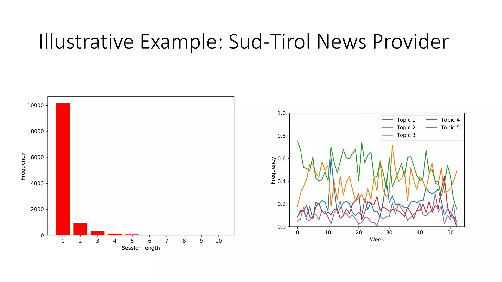
• Useful in applications in which seasonal/evolving distributions might be
observed (also referred as concept drift in ML) [Žliobaitė et al., 2016]
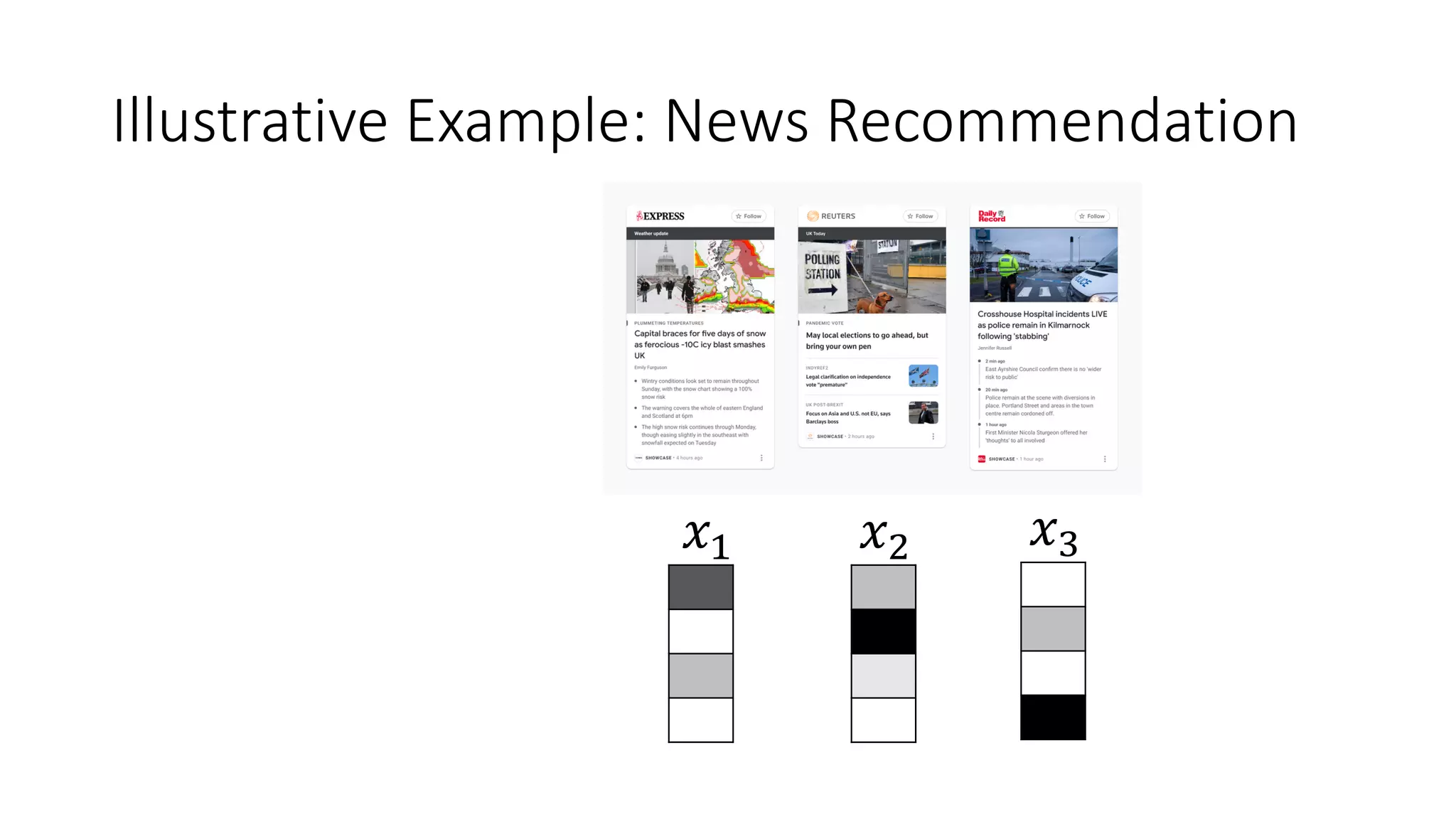
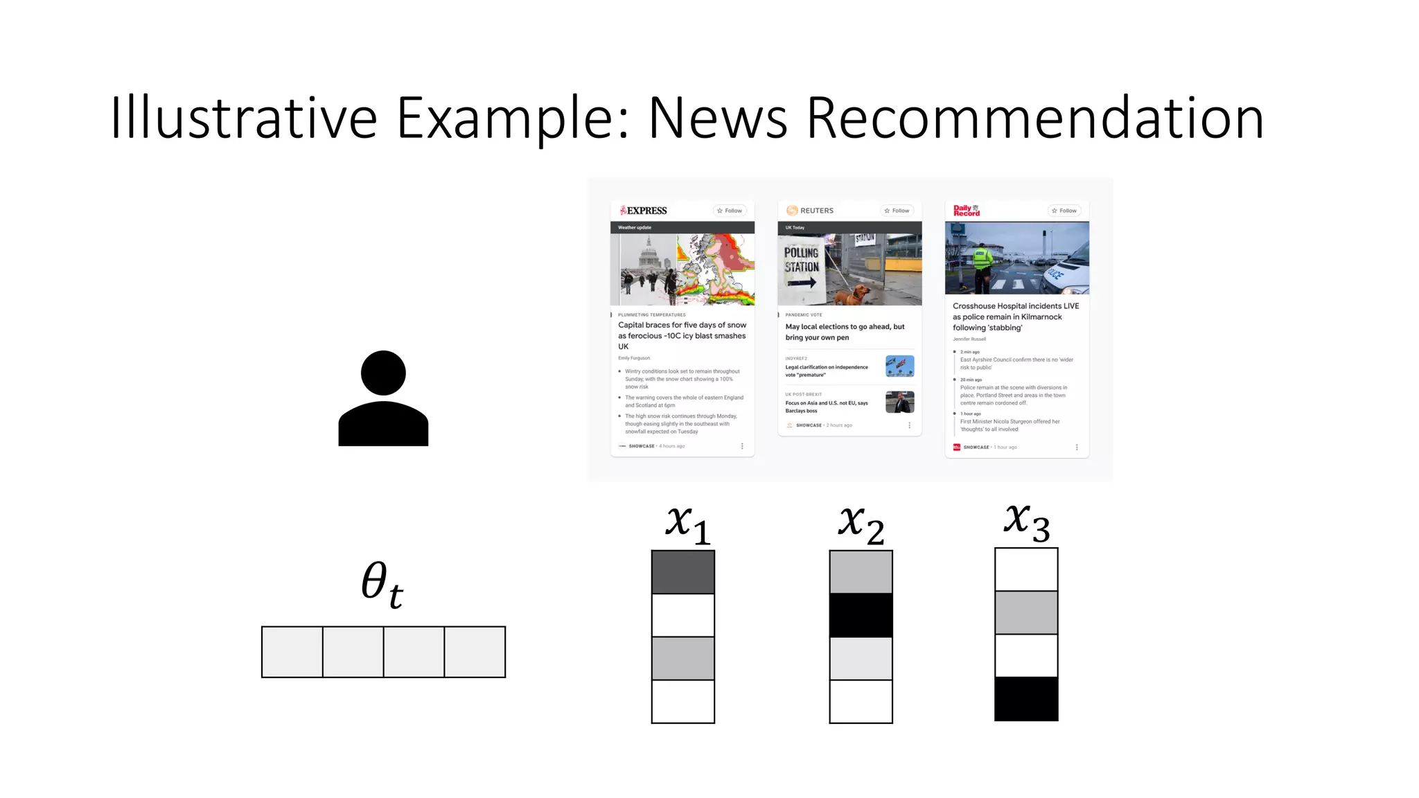
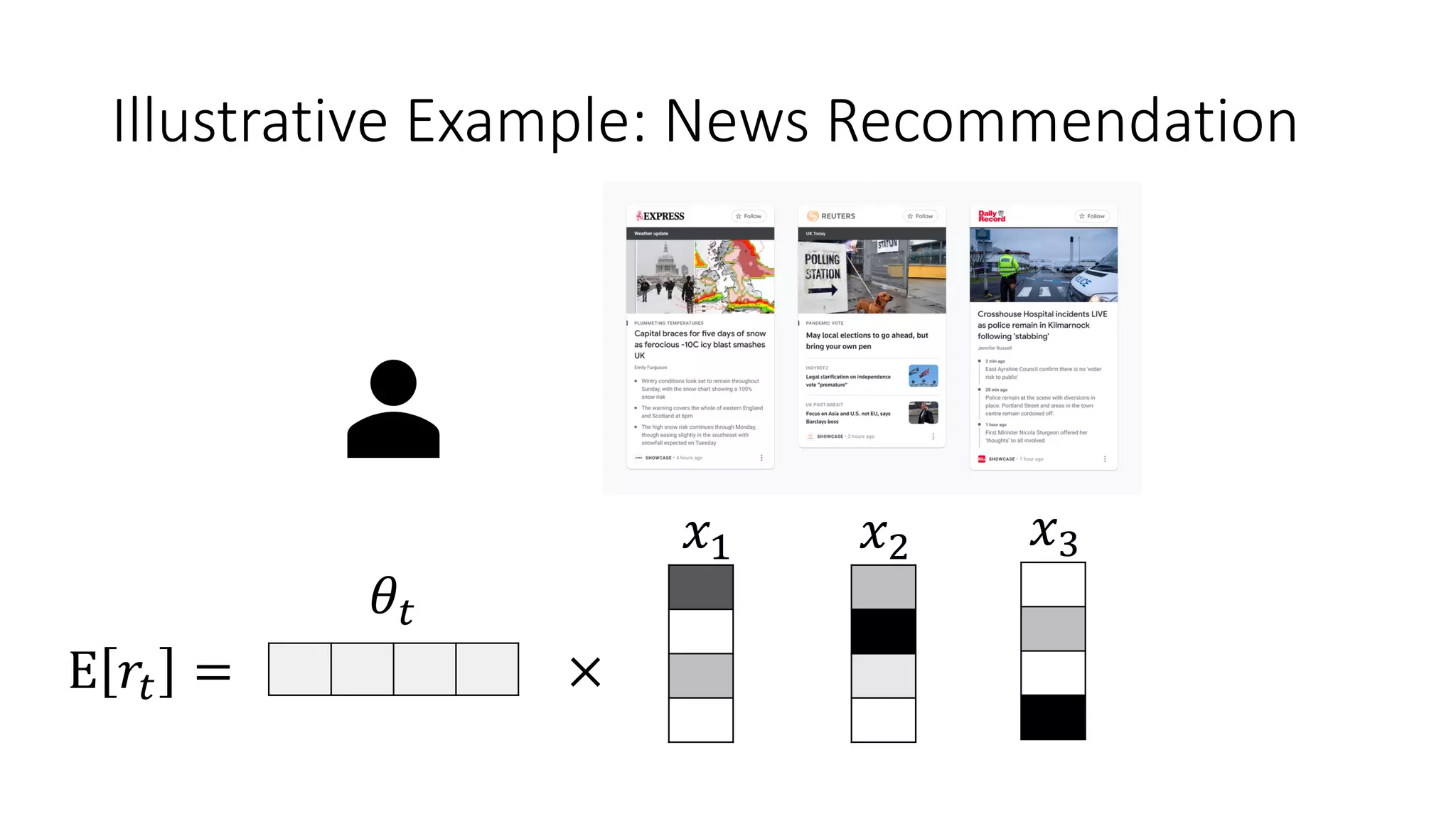
• e.g., Short-session news recommendation
• Few interactions per users (no data for personalization)
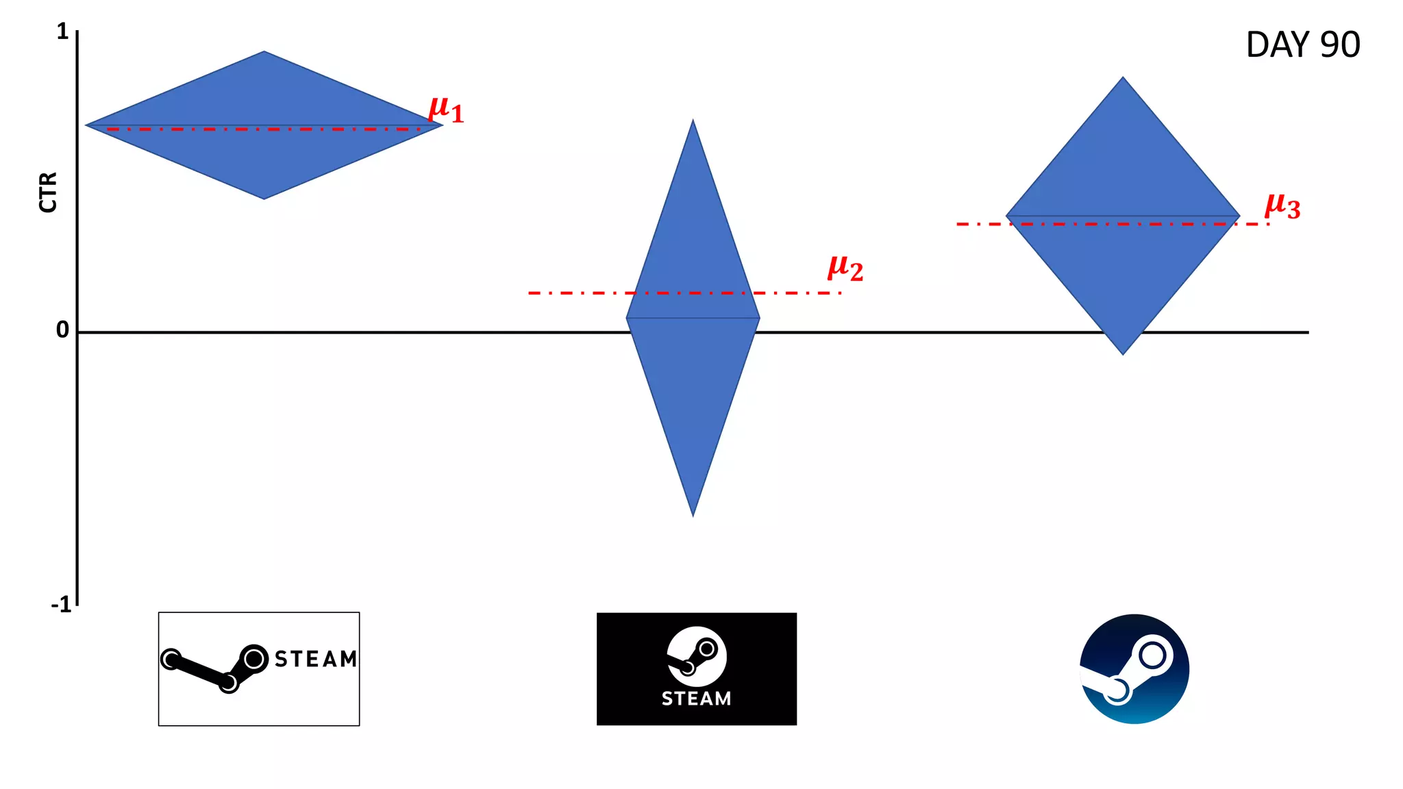
• Rapidly evolving trends (i.e., topic distributions) over the days

46. Illustrative Example: Sud-Tirol News Provider

47. Discounted TS
[Raj & Kalyani, 2017]

48. Discounted TS
[Raj & Kalyani, 2017]
𝛾 factor of discount for older rewards

49. Sliding-Window TS
[Trovò et al., 2020]

50. Sliding-Window TS
Consider only last 𝜏 rewards when
computing ℬ parameters
[Trovò et al., 2020]

51. f-Discounted
Sliding-Window TS
[Cavenaghi et al., 2021]

52. f-Discounted
Sliding-Window TS
Historic trace with discounted rewards
[Cavenaghi et al., 2021]

53. f-Discounted
Sliding-Window TS
Hot trace with sliding window
[Cavenaghi et al., 2021]

54. f-Discounted
Sliding-Window TS
• Two samples for each arm at t
• Historic discounted trace
• Sliding-window hot trace
• Combination of the two
parameters via an aggregation
function f (e.g., min, max,
mean)
[Cavenaghi et al., 2021]

55. Simulated Decreasing Reward (environment)
[Cavenaghi et al., 2021]

56. Simulated Decreasing Reward (reward/regret)
[Cavenaghi et al., 2021]

57. Comparison on Real-World Data
[Cavenaghi et al., 2021]
More experiments and details in the paper @ https://www.mdpi.com/1099-4300/23/3/380
Open-source code @ https://github.com/CavenaghiEmanuele/Multi-armed-bandit

58. More Advanced Methods
• Change-point detection UCB [Liu et al., 2018]
• Concept drift sliding-window with TS [Bifet & Gavalda, 2007]
• Burst-induced MAB [Alves et al., 2021]
• ...

59. CONTEXTUAL MAB

60. Introducing Context: Motivation
• The action a might not be equally appealing at each time step t ->
contextual conditions might change
• Actions can be inter-dependent
• It could be useful to represent those contextual conditions, i.e., define
the features of the actions or the agent/environment
• Introducing a context 𝒙 ∈ ℛ3
formalizing the contextual conditions:
• You might consider the context as a feature vector of length d
• The expected reward for arm a is now computed by the dot product of the
hidden (estimated) parameter vector 𝜽𝒕 and the context vector 𝒙𝒕,𝒂
E 𝑟#,' 𝑥#,' = 𝒙𝒕,𝒂𝜽𝒕

61. Illustrative Example: News Recommendation

62. Illustrative Example: News Recommendation
𝑥! 𝑥" 𝑥#

63. Illustrative Example: News Recommendation
𝜃$
𝑥! 𝑥" 𝑥#

64. Illustrative Example: News Recommendation
E 𝑟$ = ×
𝜃$
𝑥! 𝑥" 𝑥#

65. Illustrative Example: News Recommendation
E 𝑟$ = ×
𝜃$
𝑥! 𝑥" 𝑥#

66. Illustrative Example: News Recommendation
E 𝑟$ = ×
𝜃$
𝑥! 𝑥" 𝑥#

67. Illustrative Example: News Recommendation
𝜃$
𝑥! 𝑥" 𝑥#

68. Thompson Sampling
[Agrawal & Goyal, 2013]

69. Thompson Sampling
We sample from a multivariate Gaussian distribution
with mean vector )
𝝁 and covariance matrix 𝑩!"
[Agrawal & Goyal, 2013]

70. Thompson Sampling
[Agrawal & Goyal, 2013]
We assume an underlying unknown parameter 𝝁∗
,
which is approximated by 𝒖𝒕 , such that the expected
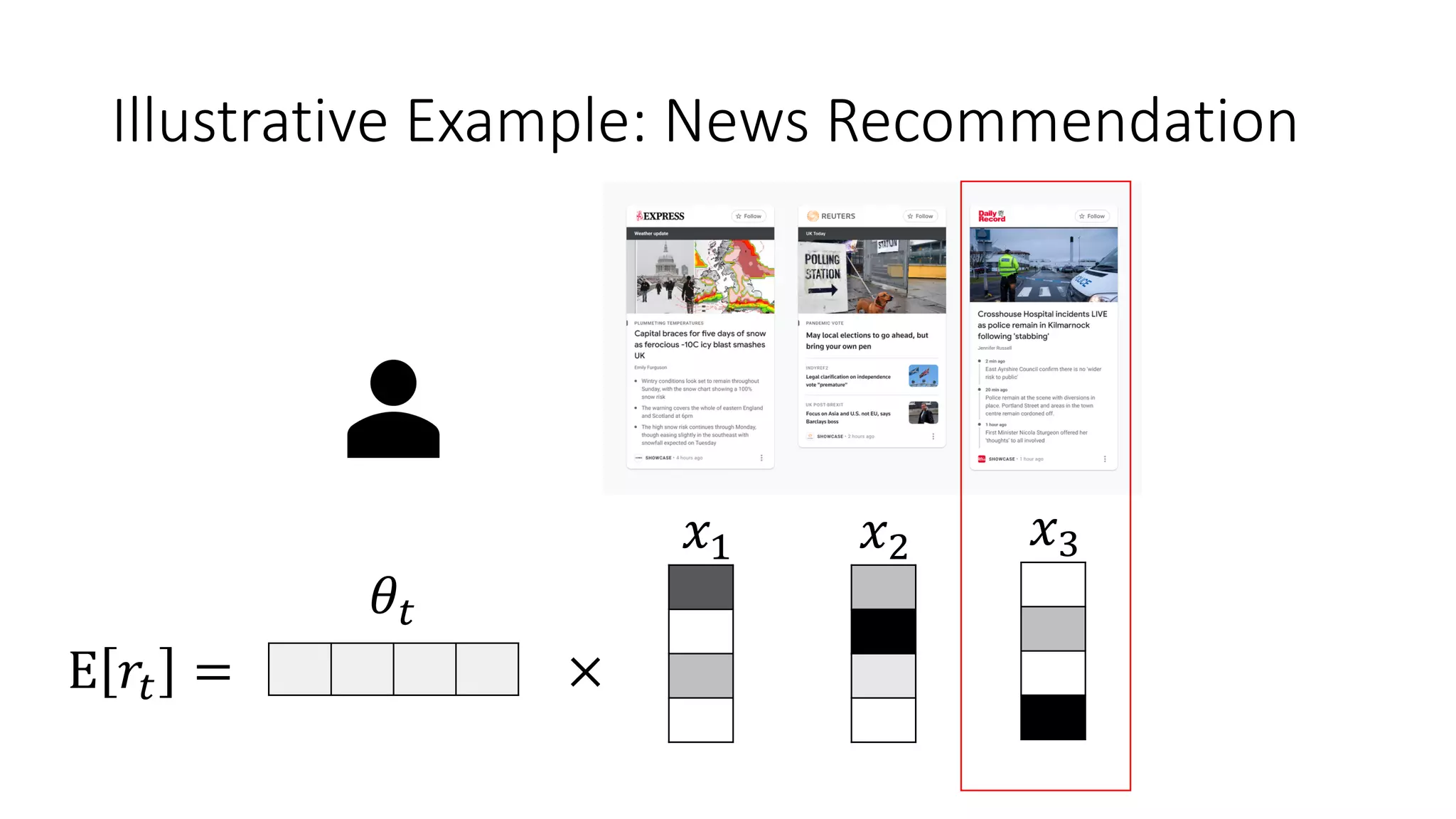
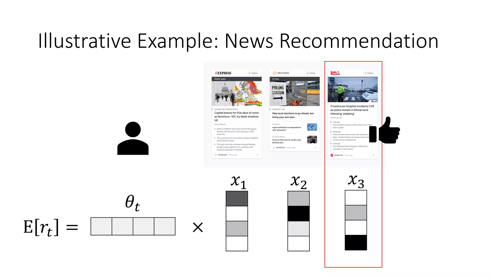
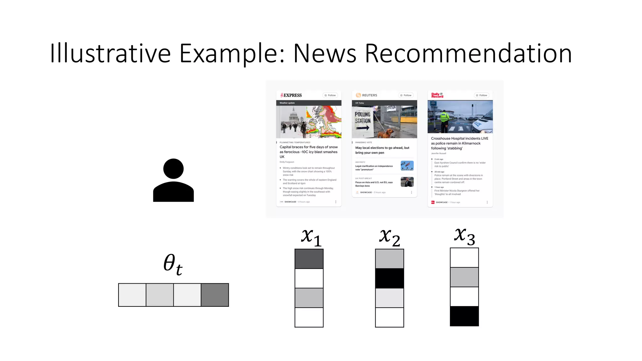
reward is a linear combination E 𝑟%,' = 𝒙𝒕,𝒂 𝝁∗

71. Thompson Sampling
[Agrawal & Goyal, 2013]
Parameters update based on given context
𝒙𝒕,𝒂 and reward rt following Ridge Regression

72. Linear Upper Confidence Bound
[Li et al., 2010]

73. Linear Upper Confidence Bound
[Li et al., 2010]

74. Linear Upper Confidence Bound
[Li et al., 2010]

75. Case Study: Conversational Picture-based DSSApple
• Apple is the third most produced fruit worldwide (86+ million metric tons in
2019), apple exports are valued 7+ billion USD
• Problem: Post-harvest disease, occurring during storage, is one of the main
causes of economic losses for apples production (10% in integrated – 30% in
organic)
• Goal: Develop a Decision Support System (DSS) fully based on user
interaction with symptom images to guide the diagnosis of post-harvest
diseases of apples
[Sottocornola et al., 2020]

76. Case Study: Conversational Picture-based DSSApple
[Sottocornola et al., 2020]

77. Case Study: Conversational Picture-based DSSApple

78. Case Study: Conversational Picture-based DSSApple

79. Case Study: Conversational Picture-based DSSApple
• How to reload the set of images in subsequent round?
• We want to adapt images reloading based on past feedback of the user BUT…
• …Similar images may belong to different diseases – User can be easily mistaken and
provide wrong feedback to similar diseases
• We focus on symptom images features (extracted through PCA)
• Rationale: implement a conversational sampling strategy that applies both
exploitation (rely on user previous feedback) and exploration (show the most
diverse set of images) -> Contextual Multi-Armed Bandit

80. Case Study: Conversational Picture-based DSSApple
• Unknown parameter 𝜇∗ represents the user “preferences” w.r.t. the
contextual features of the images (e.g., spots, spores, rotten shape, etc.)
• Parameter 𝜇% is sampled at round t from a Gaussian multivariate
distribution with expected value ̂
𝜇%
• The expected reward for each image is the dot product of the estimated
user preference 𝜇% and the image context 𝑏$
• The image to show next is iteratively selected by maximizing the expected
reward 𝑎% = argmax
$
𝑏$𝜇%
• Within a round, feedback (= reward) is collected over different images
• A selected image represents a positive reward
• Not selecting an image is a (slightly) negative reward
• The feedback allows to refine the estimation of ̂
𝜇%

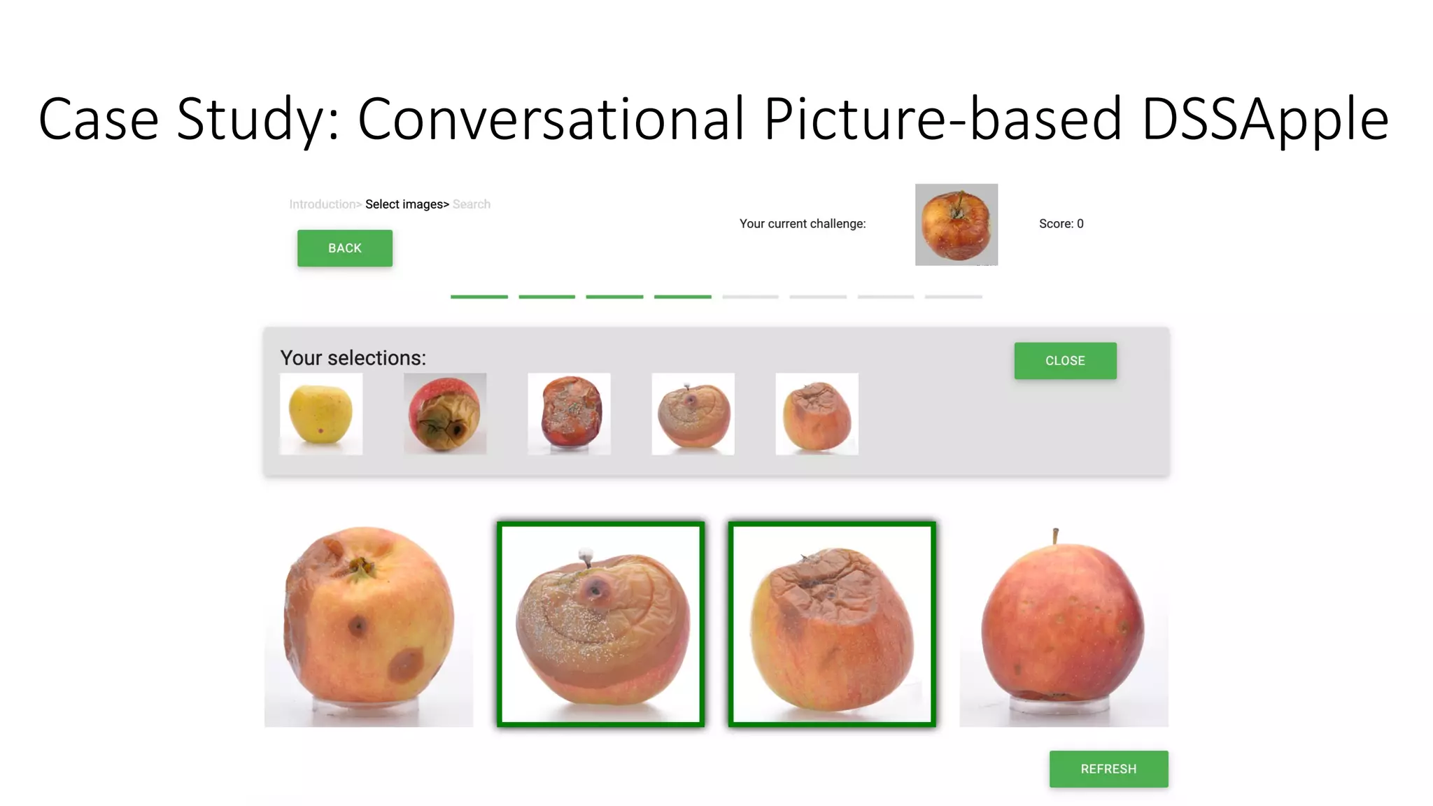
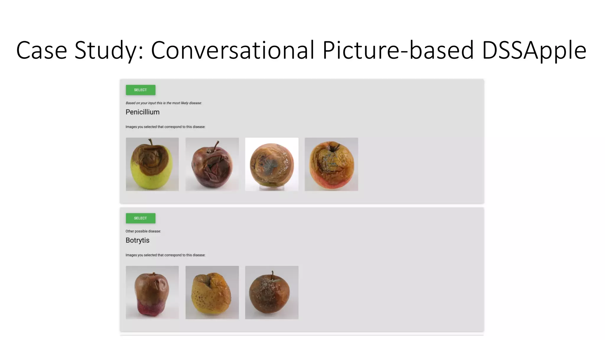
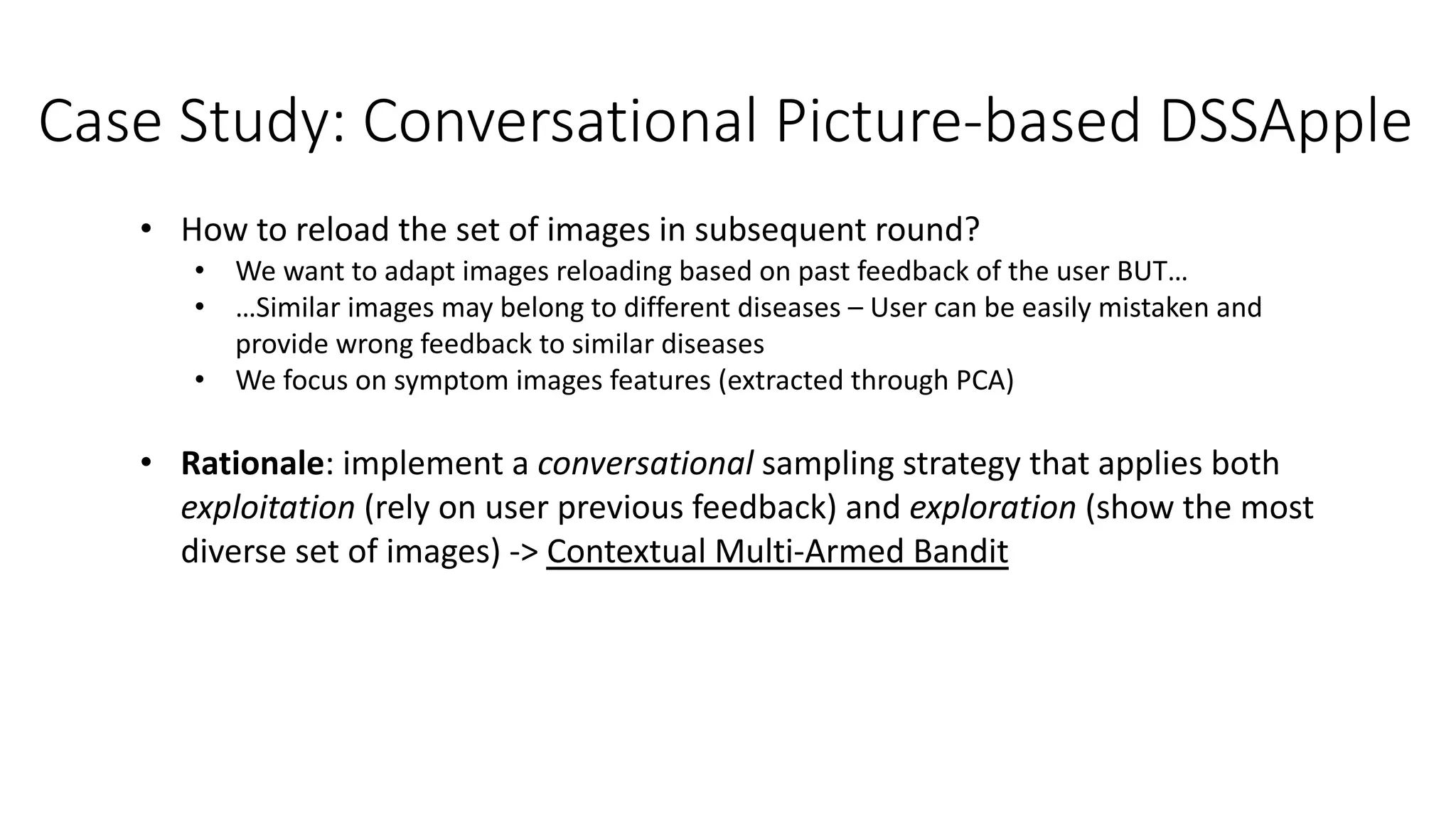
81. Case Study: Conversational Picture-based DSSApple
• Gamified challenge with 163
BSc CS students performing
515 diagnoses
• 8 rounds with 4 images
• 5 diseases to be selected
• 4 different strategies of
reloading are implemented:
• Stratified Random (total
exploration)
• Greedy (total exploitation)
• Upper Confidence Bound
• Thompson sampling
[Sottocornola et al., 2021a]

82. COUNTERFACTUAL MAB WITH
UNOBSERVED CONFOUNDERS

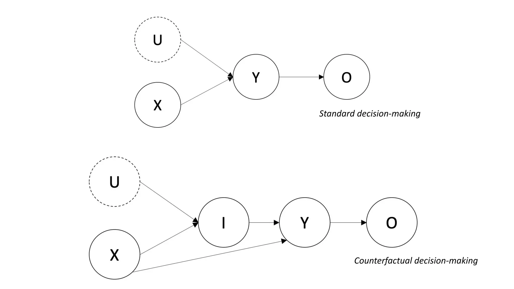
83. Preliminaries
• Unobserved Confounders: factors U that simultaneously affect the
treatment/action (i.e., the arm selection) and the outcome (i.e., the bandit
reward), but are not accounted in the analysis
• Counterfactual: Let X be the set of player’s choice and Y the set of
outcomes. The counterfactual sentence “Y would be y (in situation U = u),
had X been x, given that X = x’ was observed” is interpreted as the causal
equation Yx(u) = y
[Bareinboim et al., 2015]

84. Illustrative Example: Greedy Casino
• Two models of slot machines (M1 and M2), which learned the habits of the
players to adapt their payoff and increase casino outcome
• Player “natural” choice of the machine 𝑋 ∈ {𝑀2, 𝑀3} is a function of player
inebriation 𝐷 ∈ {0,1} and whether machine is blinking 𝐵 ∈ 0,1
• 𝑋 ← 𝑓" 𝐷, 𝐵 = 𝐷⨁𝐵
• Every player has equal chance to be inebriated, as well as every machine has equal
chance to be blinking 𝑃 𝐷 = 0 = 𝑃 𝐷 = 1 = 𝑃 𝐵 = 0 = 𝑃 𝐵 = 1 = 0.5
• Slot machines have full knowledge of the environment and adapt their payoff
according to player’s natural choice
[Bareinboim et al., 2015]
(a) Payoff rates and player natural choice (*), (b) Observational and Experimental expected reward

85. Illustrative Example: Greedy Casino
• Greedy casino meets legal requirement of providing a payoff of 30% (under
randomized control trial), while in practice (under observational model) it is
paying just 15% of the times!
• Run a set of bandit/randomized experiments to improve the performance of
the players
[Bareinboim et al., 2015]

86. MABUC Policy
• Exploit effect of the treatment of the treated (i.e., counterfactual) to include
unobserved confounders in the expected reward computation
• From average reward across arms (standard bandit) E(𝑌|𝑑𝑜 𝑋 = 𝑎 )
• To average reward by choosing and action w.r.t. natural choice (intuition)
E(𝑌456|𝑋 = 𝑎)
• Regret decision criterion: counterfactual nature of the inference, i.e.,
interrupt any reasoning agent before executing their choice, treat this as an
intention, compute the counterfactual expectation, then act.
[Bareinboim et al., 2015]

87. Causal Thompson Sampling
[Bareinboim et al., 2015]

88. Causal Thompson Sampling
[Bareinboim et al., 2015]

89. Causal Thompson Sampling
[Bareinboim et al., 2015]

90. Causal Thompson Sampling
[Bareinboim et al., 2015]

91. Case Study: CF-CMAB to DSSApple Diagnosis
[Sottocornola et al., 2021b]

92. • Idea: Leverage past user interactions (and decisions) with DSSApple
application to sequentially boost diagnosis accuracy including unobserved
confounders U
• Counterfactual Thompson Sampling (CF-TS) for contextual diagnosis: linear
CMAB (with TS policy) for “disease classification”, enhanced with
counterfactual computation on user decision
• Context: User feedback X provided to the system during a session of
diagnosis (i.e., images clicked as similar)
• Counterfactual: Regret decision criterion, i.e., interrupt users as they
execute their decision (i.e., diagnosis), treat this as an intuition I and
compute counterfactual decision Y
Counterfactual Contextual MAB
[Sottocornola et al., 2021b]

93. Standard decision-making
Counterfactual decision-making

94. CF-TS Algorithm
• At time t, play arm
• Expected reward is computed as
• In causal terms, this corresponds to optimize the expected outcome 𝑂 for
selecting arm 𝑌 = 𝑦, given the contextual information 𝑋 = 𝑥𝑡 and the
intuition of the user towards arm 𝐼 = 𝑖𝑡
• “What have been the expected reward had I pull arm 𝑦 given that I am
about to pull arm 𝑖𝑡 ?”
[Sottocornola et al., 2021b]

95. CF-TS Algorithm
[Sottocornola et al., 2021b]

96. CF-TS Algorithm
[Sottocornola et al., 2021b]

97. Case Study: DSSApple Diagnosis Results
[Sottocornola et al., 2021b]
Cumulative reward for the image-based context (a) and the similarity-based context (b)

98. Case Study: DSSApple Diagnosis Results
[Sottocornola et al., 2021b]
Open-source code @ https://github.com/endlessinertia/causal-contextual-bandits

99. References
• [Auer et al., 2002] Auer, P., Cesa-Bianchi, N., & Fischer, P. (2002). Finite-time analysis of the multiarmed bandit problem. Machine
learning, 47(2), 235-256.
• [Shahriari et al., 2015] Shahriari, B., Swersky, K., Wang, Z., Adams, R. P., & De Freitas, N. (2015). Taking the human out of the loop: A
review of Bayesian optimization. Proceedings of the IEEE, 104(1), 148-175.
• [Jeunen & Goethals, 2021] Jeunen, O., & Goethals, B. (2021). Pessimistic reward models for off-policy learning in recommendation.
In Fifteenth ACM Conference on Recommender Systems (pp. 63-74).
• [Raj & Kalyani, 2017] Raj, V., & Kalyani, S. (2017). Taming non-stationary bandits: A Bayesian approach. arXiv preprint
arXiv:1707.09727.
• [Trovò et al., 2020] Trovò, F., Paladino, S., Restelli, M., & Gatti, N. (2020). Sliding-window thompson sampling for non-stationary
settings. Journal of Artificial Intelligence Research, 68, 311-364.
• [Cavenaghi et al., 2021] Cavenaghi, E., Sottocornola, G., Stella, F., & Zanker, M. (2021). Non Stationary Multi-Armed Bandit:
Empirical Evaluation of a New Concept Drift-Aware Algorithm. Entropy, 23(3), 380.
• [Liu et al., 2018] Liu, F., Lee, J., & Shroff, N. (2018). A change-detection based framework for piecewise-stationary multi-armed
bandit problem. In Proceedings of the AAAI Conference on Artificial Intelligence (Vol. 32, No. 1).
• [Bifet & Gavalda, 2007] Bifet, A., & Gavalda, R. (2007). Learning from time-changing data with adaptive windowing. In Proceedings
of the 2007 SIAM international conference on data mining (pp. 443-448). Society for Industrial and Applied Mathematics.
• [Alves et al., 2021] Alves, R., Ledent, A., & Kloft, M. (2021). Burst-induced Multi-Armed Bandit for Learning Recommendation.
In Fifteenth ACM Conference on Recommender Systems (pp. 292-301).

100. References
• [Agrawal & Goyal, 2013] Agrawal, S., & Goyal, N. (2013). Thompson sampling for contextual bandits with linear payoffs.
In International Conference on Machine Learning (pp. 127-135). PMLR.
• [Li et al., 2010] Li, L., Chu, W., Langford, J., & Schapire, R. E. (2010). A contextual-bandit approach to personalized news article
recommendation. In Proceedings of the 19th international conference on World wide web (pp. 661-670).
• [Sottocornola et al., 2020] Sottocornola, G., Nocker, M., Stella, F., & Zanker, M. (2020). Contextual multi-armed bandit strategies for
diagnosing post-harvest diseases of apple. In Proceedings of the 25th International Conference on Intelligent User Interfaces (pp.
83-87).
• [Sottocornola et al., 2021a] Sottocornola, G., Baric, S., Nocker, M., Stella, F., & Zanker, M. (2021). Picture-based and conversational
decision support to diagnose post-harvest apple diseases. Expert Systems with Applications, 116052.
• [Bareinboim et al., 2015] Bareinboim, E., Forney, A., & Pearl, J. (2015). Bandits with unobserved confounders: A causal
approach. Advances in Neural Information Processing Systems, 28, 1342-1350.
• [Sottocornola et al., 2021b] Sottocornola, G., Stella, F., & Zanker, M. (2021). Counterfactual Contextual Multi-Armed Bandit: a Real-
World Application to Diagnose Apple Diseases. arXiv preprint arXiv:2102.04214.
• [Žliobaitė et al., 2016] Žliobaitė, I., Pechenizkiy, M., & Gama, J. (2016). An overview of concept drift applications. Big data analysis:
new algorithms for a new society, 91-114.