Introduction

1. Computer Graphics & Linear Algebra
Gabrien Clark
May 5, 2010
Computer Graphics
1 Introduction
The area of computer graphics is a vast and ever expanding field. In the
simplest sense computer graphics are images viewable on a computer screen.
Applications extend into such processes as engineering design programs and
almost any type of media. The images are generated using computers and
likewise, are manipulated by computers. Underlying the representation of
the images on the computer screen is the mathematics of Linear Algebra.
We will explore the fundamentals of how computers use linear algebra to
create these images, and branch off into basic manipulation of these images.
2 2-Dimensional Graphics
Examples of computer graphics are those of which belong to 2 dimensions.
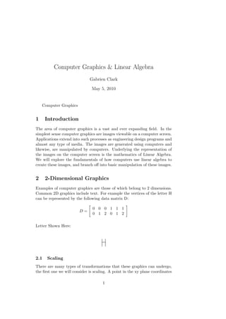
Common 2D graphics include text. For example the vertices of the letter H
can be represented by the following data matrix D:
D =
0 0 0 1 1 1
0 1 2 0 1 2
Letter Shown Here:
2.1 Scaling
There are many types of transformations that these graphics can undergo,
the first one we will consider is scaling. A point in the xy plane coordinates
1

2. are given by (x,y) or A=
X
Y
.
The scaling transformation is given by the matrix S=
C1 0
0 C2
. Where
the Cis are scalars. The scaling transforms the coordinates (x,y) into (C1x,
C2y). In mathematical terms the transformation is given by the multiplica-
tion of the matrices S and A:
S A =
C1 0
0 C2
X
Y
=
C1X
C2Y
Example: Now let’s examine how scaling affects our example H. Let C1=2
and C2=2, our new coordinates for D are:
D =



0 0 0 2 2 2
0 2 4 0 2 4
0 0 0 0 0 0



The new H is now twice as long in the X-direction and twice as long in the
Y-direction.
Now that we have examined the scaling transformation, let’s move on to
the other two basic transformations that underly the movement of a figure
on a computer screen, translating and rotating.
2.2 Translation
Let’s revisit our example matrix A with coordinates (X,Y,1) or



X
Y
1


. The
post-translational coordinates of A can be obtained by multiplying A by the
matrix I T , where I represents the I3 Identity Matrix, and T represents
the column vector containing the translation coordinates for A. Mathemat-
ically speaking translation is represented by:
I T



X
Y
1


 =



1 0 X0
0 1 Y0
0 0 1






X
Y
1


 =



X+X0
Y +Y0
1



Example: Let us now revisit our example letter and H and show how it is
affected by an arbitrary translation. Let us set our arbitrary translational
vector to T=



2
3
1


, then I T =



1 0 2
0 1 3
0 0 1


, and the final matrix can
be given by:
2

3. I T D =



2 2 2 3 3 3
3 4 5 3 4 5
0 0 0 0 0 0



Our examle letter H has now moved 2 units in the positve X-direction
and 3 units in the positive Y-direction.
2.3 Rotation
Next, we have the transformation of rotation. A more complex transfor-
mation, rotation changes the orientation of the image about some axis,
in our case either X or Y. Clockwise rotations have the rotational matrix
R(−θ) =



cos(θ) −sin(θ) 0
sin(θ) cos(θ) 0
0 0 1


, but all rotational matrices are given in a
variation of the form of the rotational matrix for counter-clockwise rotation
R(θ) =



cos(θ) −sin(θ) 0
sin(θ) cos(θ) 0
0 0 1


. The counter-clockwise rotation of matrix
A is given by:
R(θ) A =



cos(θ) −sin(θ) 0
sin(θ) cos(θ) 0
0 0 1






X
Y
1



=



XCos(θ) − Y Sin(θ)
XSin(θ) + Y Cos(θ)
1



Example: Now let us visually examine a rotation of 90◦ of our example
letter H:
Mathematically speaking the rotation of 90◦occurs when θ = π/2. So now
we can view the mathematics that made this transformation possible:
R(θ) D =



cos(π/2) −sin(π/2) 0
sin(π/2) cos(π/2) 0
0 0 1






0 0 0 1 1 1
0 1 2 0 1 2
0 0 0 0 0 0


 =



0 −1 0
1 0 0
0 0 0






0 0 0 1 1 1
0 1 2 0 1 2
0 0 0 0 0 0


 =
3

4. 


0 −1 −2 0 −1 −2
0 0 0 1 1 1
0 0 0 0 0 0



If we refer to both the earlier visualization and mathematical display we
see that letter H has been rotated 90◦about the origin.
2.4 Composite Transformations
Now that we have gone over these basic transformations, it is now time to
combine them to examine the net result of how multiple transformations
affect an image,movement. Movement of the image is caused by the multi-
plication of the scaling, translational, rotational, and other transformational
matrices with the coordinate matrix. The result of these matrix multipli-
cations are called Composite Transformations. To finish up our view in the
world of 2-Dimensional graphics, lets mathematically examine a composite
transformation of our example letter H using the scaling, translational, and
rotational matrices we’ve already established. The composite transfomation
of H can be represented by:
S T R(θ) D =



2 0 0
0 2 0
0 0 0






1 0 2
0 1 3
0 0 1






0 −1 0
1 0 0
0 0 0






0 0 0 1 1 1
0 1 2 0 1 2
0 0 0 0 0 0


=



0 −2 −4 0 −2 −4
0 0 0 20 20 20
0 0 0 0 0 0



3 3-Dimensional Graphics
Now that we’ve effectively explored the region of 2-Dimensional, we can be-
gin to explore the region of 3-Dimensional graphics. 3-Dimensional graphics
live in R3 versus 2-Dimensional graphics which live in R2. 3-Dimensional
graphics have a vast deal more applications in comparison to 2-Dimensional
graphics, and are, likewise, more complicated. We will now work with the
variable Z, in addition to X and Y, to fully represent coordinates on the X,
Y, and Z axes, or simply space.
Homogeneous 3-Dimensional Coordinates For every point (X,Y,Z,) in
R3, there exists a point (X,Y,Z,1) on the R4 plane. We call the second pair
of coordinates Homogeneous Coordinates. (Note: Homogeneous coordinates
4

5. can not be added or multiplied by scalars. In R3 they may only be multi-
plied by 4x4 matrices.) If H= 0, then :
• X = x
H
• Y = y
H
• Z = z
H
We now call (x,y,z,H) homogeneous coordinates for (X,Y,Z) and (X,Y,Z,1)
Example: Find homogeneous coordinates for the point (4,2,7)
Solution:
Refer to our earlier equations for finding the coordinates (x,y,z). Let’s
show two solutions for the question.
Solution 1: Let H = 1
2:
x = 4
1
2
= 8, y = 2
1
2
= 4, z = 7
1
2
= 14
(x, y, z)=(8, 4, 14)
Solution 2: Let H=2:
x = 4
2 = 2, y = 2
2 = 1, z = 7
2 = 3.5
(x, y, z)=(2, 1, 3.5)
3.1 Visualization
When we view 3-Dimensional objects on computer screens, we do not
actually see the images themselves, but rather we see projections of
these objects onto the viewing plane, or computer screen. The object
we see is determined by a set amount of straight line segments, whose
endpoints P1, P2, P3,..., Pn are represented by coordinates (x1, y1, z1),
5

6. (x2, y2, z2), (x3, y3, z3), ..., (xn, yn, zn). These line segments and co-
ordinates are placed in the memory of a computer. The corresponding
coordinate matrix can be represented by:
P=



X1 X2 . . . Xn
Y1 Y2 . . . Yn
Z1 Z2 . . . Zn



3.1.1 Perspective Projection
Let’s assume that a 3-Dimensional object displayed on a computer screen
is being mapped onto the XY-plane. We say that a perspective projec-
tion maps each point (x,y,z) onto an image point (x∗, y∗, 0). We call the
point where the image’s coordinates, it’s projected coordinates, and the eye
position meet the center of projection.
Example: Using homogeneous coordinates represent the perspective pro-
jection of the matrix P.
Solution: If we scale the coordinates by 1
1− z
d
, then (x, y, z, 1)−→ (x1− z
d
,
y
1− z
d
, 0, 1)
Now we can represent P as:
P





x
y
z
1





=





1 0 0 0
0 1 0 0
0 0 0 0
0 0 −110 1










x
y
z
1





=





x
y
0
11− z
d





3.2 Scaling
In 3-Dimensions, scaling moves the coordinates (X,Y,Z) to new coordinates
(C1, C2, C3) where the C −is are scalars. Scaling in 3-Dimensions is exactly
like scaling in 2-Dimensions, except that the scaling occurs along 3 axes,
rather than 2. Note that if we view strictly from the XY-plane the scaling
in the Z-direction can not be seen, if we view strictly from the XZ-plane the
scaling in the Y-direction can not be seen, and if we view strictly from the
YZ-plane then the scaling in the X-direction can not be seen. The scaling
matrix in 3-Dimension is represented by:
6

7. S=



C1 0 0
0 C2 0
0 0 C3



The scaling transformation, like in 2-Dimensions, is represented by the ma-
trix multiplication of the Scaling Matrix and coordinate matrix A:
S A =



C1 0 0
0 C2 0
0 0 C3






X
Y
Z


 =



C1X
C2Y
C3Z



Example: Give the matrix for a scaled cube with original coordinates
given by A=



0 0 0 0 2 2 2 2
0 2 2 0 0 2 2 0
0 0 −2 −2 0 0 −2 −2


, and the scaling matrix is
given by S=



1 0 0
0 2 0
0 0 3



Solution:
S A =



1 0 0
0 2 0
0 0 3






0 0 0 0 2 2 2 2
0 2 2 0 0 2 2 0
0 0 −2 −2 0 0 −2 −2



=



0 0 0 0 2 2 2 2
0 4 4 0 0 4 4 0
0 0 −6 −6 0 0 −6 −6



From calculating the new matrix we can see that the cube isn’t scaled in the
X-direction, scaled to twice it’s size in the positive Y-direction, and scaled
to triple it’s size in the negative Z-direction.
3.3 Translation
Like scaling, Translation is exactly the same in space as in 2-Dimensions,
with the exception of the use of the Z-axis. If we were to view a trans-
lating object moving in either the positve or negative Z-direction strictly
from the perspective of the XY-plane, then it would appear to us that im-
age is increasing or decreasing, respectively, in size. In reality this is just
how the computer establishes the object is translating in space. This also
applies for the other directions with respect to the other planes. Translation
7

8. in 3-dimensions is represented by the matrix multiplication of the transla-
tion vector T=





1 0 0 X0
0 1 0 Y0
0 0 1 Z0
0 0 0 1





, and the coordinate matrix A=





X
Y
Z
1





.
Mathematically speaking we can represent the 3-Dimensional translation
transformation with:
T A =





1 0 0 X0
0 1 0 Y0
0 0 1 Z0
0 0 0 1










X
Y
Z
1





=





X+X0
Y +Y0
Z+Z0
1





Example: Give the matrix for the translation of a point (5, 3, -8, 1) by
the vector p=(-4, -6, 3)
Solution: The matrix that maps (X, Y, Z, 1) −→ (X − 4, Y − 6, Z + 3, 1) is
given by I T =





1 0 0 −4
0 1 0 −6
0 0 1 3
0 0 0 1





, A=





5
3
−8
1





, so :
I T A =





1 0 0 −4
0 1 0 −6
0 0 1 3
0 0 0 1










5
3
−8
1





=





1
−3
−5
1





3.4 Rotation
We finally arrive at rotation in 3-Dimensions. Just like scaling and translat-
ing, rotation in three dimensions is fundamentally the same as rotation in
3-Dimensions, with the exception that we also can rotate about the Z-axis.
The rotations about the X, Y, and Z axes are given by:
• R(θ)X=



1 0 0
0 Cos(θ) −Sin(θ)
0 Sin(θ) Cos(θ)



(Rotates the y-axis towards the z-axis)
8

9. • R(θ)Y =



Cos(θ) 0 Sin(θ)
0 1 0
−Sin(θ) 0 Cos(θ)



(Rotates the z-axis towards the x-axis)
• R(θ)Z=



Cos(θ) −Sin(θ) 0
Sin(θ) Cos(θ) 0
0 0 1



(Rotates the x-axis towards the y-axis)
We can display the post-reflection coordinates as:
• R(θ)X: (X,Y,Z) −→ (X, Y Cos(θ) − ZSin(θ), ZCos(θ) + Y Sin(θ))
• R(θ)X: (X,Y,Z) −→ (XCos(θ) + ZSin(θ), Y, −XSin(θ) + ZCos(θ))
• R(θ)X: (X,Y,Z) −→ (XCos(θ) − Y Sin(θ), Y Cos(θ) + XSin(θ), Z)
Example: Give the final Rotational Matrix, R, for an image that is first
rotated about the X-axis 47◦, then about the Y-axis 52◦, and then about
the Z-axis -30◦.
Solution: R can be mathematically represented by the matrix multiplica-
tions of the 3 rotational matrices of the X, Y, and Z axes. Mathematically
speaking:
R= R(θ)X R(θ)Y R(θ)Z
=



1 0 0
0 Cos(θ) −Sin(θ)
0 Sin(θ) Cos(θ)






Cos(θ) 0 Sin(θ)
0 1 0
−Sin(θ) 0 Cos(θ)






Cos(θ) −Sin(θ) 0
Sin(θ) Cos(θ) 0
0 0 1



=



1 0 0
0 Cos(47◦) −Sin(47◦)
0 Sin(47◦) Cos(47◦)






Cos(52◦) 0 Sin(52◦)
0 1 0
−Sin(52◦) 0 Cos(52◦)






Cos(−30◦) −Sin(−30◦) 0
Sin(−30◦) Cos(−30◦) 0
0 0 1



=



.533 .308 .788
.158 .879 −.450
−.831 .365 .420



9

10. 4 Conclusion
Today we have only scratched the surface of the world of computer graphics.
The advancement of computer grahics has made technology more functional
and user-friendly. Mainstream applications of computer graphics can be seen
in every type of media including animation, movies, and video games. The
breadth of computer graphics range from basic pixel art and vector graphics
to the incredibly realistic animation of high end 3D gaming programs, such
as games typically played on Microsoft c Xbox 360. Applications of these
graphics also extend into the world of science. Currently biologists are using
computer grapchis for molecular modeling. Through these crucial visualiza-
tions scientists are able to make advances in drug and cancer research, that
otherwise would not be possible. A major future application of computer
graphics lies in the domain of virtual reality. In vitual reality one is able to
experience a synthesized computer environment just as if it were a natural
environment. It would appear that "the sky is the limit" for the world of
computer graphics, but at the basis of it all lies the mathematics of linear
algebra.
5 References
Lay, David C. Linear Algebra and Its Applications. Boston: Addison Wesley,
2003. Print.
Anton, Howard. Elementary Linear Algebra. New York: John Wiley, 1994.
657-65. Print.
Wikipedia contributors. "Computer graphics." Wikipedia, The Free Ency-
clopedia. Wikipedia, The Free Encyclopedia, 3 May. 2010. Web. 4 May.
2010.
Wikipedia contributors. "Rotation matrix." Wikipedia, The Free Encyclo-
pedia. Wikipedia, The Free Encyclopedia, 2 May. 2010. Web. 4 May.
2010.
Jordon, H. Rep. Web. Apr.-May 2010.
<http://math.illinoisstate.edu/akmanf/newwebsite/linearalgebra/computergraphics.pdf>.
10