This document describes a project report submitted for the degree of Master of Technology in Machine Learning and Computing. The report details a study on developing an automated model for recognizing business events from online news articles. Data related to business events in domains like acquisition, vendor-supplier relationships, and jobs was crawled and preprocessed. Semi-supervised techniques were used for data labeling, and vectorization methods like bag-of-words, word embeddings, and word2vec were applied to convert text into numeric features. Ensemble classifiers and convolutional neural networks were evaluated on the datasets, with promising results.


![5
vectors disregarding the grammar and the order. Consider the following sentences
where the bag-of-words approach fails.
After drawing money from the Bank Ravi went to the river Bank.
In the bag-of-words approach there is no distinction between financial word Bank
and river Bank. This problem of capturing semantics of the word to a certain
extent overcome by word-embedding. In word embedding each word is represented
by a 100 to 300 dimensional uniformly distributed (i.e U[-1,1])random dense vector.
Word-embedding with window approach captures semantics to certain extent.
1.2.3 Data Labeling
The extracted data labeled in supervised manner were few in number. The sections
below describe the semi-supervised technique and active learning methods.
1.2.3.1 Semi-supervised Technique
The naive Bayes classifier forms the integral part in the implementation of semi-
supervised learning using naive Bayes classifier with expectation maximization to
increase the number of labeled data points (kamalNigam et al.,2006). Discussed
below is an overview of the naive Bayes classifier.
Naive Bayes classifiers are probabilistic classifiers which use the concept of Bayes
theorem. In naive Bayes classifier assumption is made that one feature is condi-
tionally independent from another feature. The modeling of a naive Bayes classifier
is described as follows:
Given a input feature vector x=(x1, x2, ...., xn)T
we need to calculate which class
does this feature vector belong to i.e. p(Yk|x1, x2, ...xn) for each k classes, where
Yk is the output variable for the kth class. Now using the concept of the Bayes
theorem we can rewrite the above probability expression as:
p(Yk|x) = p(Yk)p(x|Yk)
p(x)
where
p(Yk) = are prior probabilities for that particular class
p(x|Yk) = is the maximum likelihood estimator](https://image.slidesharecdn.com/3b17c844-45a8-4fef-a969-593e5d24747f-160105130418/85/Thesis-aligned-sc13m055-28-320.jpg)


![21
Fuzz: There is an idea that is not clear e.g.: looks like, seems like, alleged,
maybe, probably, sort of.
2.4 Description of Vectorizers
All the features extracted with the given sentence has to be converted into vectors
using vectorizers such as Count-vectorizers, TF-IDF vectorizers. The method
used to convert words to vectors is bag of words approach. Following are the two
vectorizers described below using bag of words approach.
2.4.1 Count Vectorizers
This module uses the counts of the words present within a sentence and converts
it into vectors by building the dictionary for the word to vector conversion(Harris,
1954). An illustrative of example count vectorizer is described below.
2.4.1.1 Example of Count Vectorizer
Consider the following two sentences.
a) John likes to watch movies. Mary likes movies too.
b) John also likes to watch football games.
Based on the above two sentences dictionary is constructed as follows:
{ John:1 , likes:2 , to:3 , watch:4 , movies:5 , also:6 , football:7 , games:8 , Mary:9
, too:10 }
The dictionary constructed has 10 distinct words. Using the indexes of the dictio-
nary, each sentence is represented by a 10-entry vector:
sentence1 : [1, 2, 1, 1, 2, 0, 0, 0, 1, 1]
sentence2 : [1, 1, 1, 1, 0, 1, 1, 1, 0, 0]
where each entry of the vectors refers to count of the corresponding entry in the
dictionary (this is also the histogram representation). For example, in the first
vector (which represents sentence 1), the first two entries are [1,2]. The first entry
corresponds to the word John which is the first word in the dictionary, and its
value is 1 because John appears in the first sentence 1 time. Similarly the second](https://image.slidesharecdn.com/3b17c844-45a8-4fef-a969-593e5d24747f-160105130418/85/Thesis-aligned-sc13m055-44-320.jpg)


![28
The differentiable loss function in our case is Binomial deviance loss function.
The algorithm is implemented as follows as described in (Friedman et al.,2001).
Input : training set (Xi, yi), where i = 1....n , Xi ∈ H ⊆ Rn
and yi ∈ [−1, 1]
differential loss function L(y, F(X)) which in our case is Binomial deviance loss
function defined as log(1 + exp(−2yF(X))) and M are the number of iterations .
1. Initialize model with a constant value:
F0(X) =arg min
γ
n
i=1 L(yi, γ).
2. For m = 1 to M:
(a) Compute the pseudo-responses:
rim = − ∂L(yi,F(Xi))
∂F(Xi)
F(X)=Fm−1(X)
for i = 1, . . . , n.
(b) Fit a base learnerhm(X) to pseudo-response, train the pseudo response
using the training set {(Xi, rim)}n
i=1.
(c) Compute multiplier γm by solving the optimization problem:
γm = arg min
γ
n
i=1 L (yi, Fm−1(Xi) + γhm(Xi)).
(d) Update the model: Fm(X) = Fm−1(X) + γmhm(X).
3. Output FM (X) = M
m=1 γmhm(X)
The value of the weight γm is found by an approximated newton raphson solution
given as γm = Xi∈hm
rim
Xi∈hm|rim|(2−|rim|)
3.3.2 AdaBoost Classifier
In adaBoost we assign (non-negative) weights to points in the data set which
are normalized, so that it forms a distribution. In each iteration, we generate a
training set by sampling from the data using the weights, i.e. the data point (Xi, yi)
would be chosen with probability wi, where wi is the current weight for that data
point. We generate the training set by such repeated independent sampling. After
learning the current classifier, we increase the (relative) weights of data points that
are misclassified by the current classifier. We generate a fresh training set using the
modified weights and so on. The final classifier is essentially a weighted majority](https://image.slidesharecdn.com/3b17c844-45a8-4fef-a969-593e5d24747f-160105130418/85/Thesis-aligned-sc13m055-51-320.jpg)
![29
voting by all the classifiers. The description of the algorithm as in (Freund et al.,
1995) is given below:
Input n examples: (X1, y1), ..., (Xn, yn), Xi ∈ H ⊆ Rn
, yi ∈ [−1, 1]
1. Initialize: wi(1) = 1
n
, ∀i, each data point is initialized with equal weight, so
when data points are sampled from the probability distribution the chance
of getting the data point in the training set is equally likely.
2. We assume that there as M classifiers within the Ensembles.
For m=1 to M do
(a) Generate a training set by sampling with wi(m).
(b) Learn classifier hm using this training set.
(c) let ξm = n
i=1 wi(m) I[yi=hm(Xi)] where IA is the indicator function of
A and is defined as
IA = 1 if [yi = hm(Xi)]
IA = 0 if [yi = hm(Xi)]
so ξm is the error computed due to the mth classifier.
(d) Set αm=log(1−ξm
ξm
) computed hypothesis weight, such that αm > 0 be-
cause of the assumption that ξ < 0.5.
(e) Update the weight distribution over the training set as
wi(m + 1)= wi(m) exp(αmI[yi=hm(Xi)])
Normalization of the updated weights so that wi(m+1) is a distribution.
wi(m + 1) =
wi(m+1)
i wi(m+1)
end for
3. Output is final vote h(X) = sgn( M
m=1 αmhm(x)) is the weighted sum of all
classifiers in the ensemble.
In the adaboost algorithm M is a parameter. Due to the sampling with weights,
we can continue the procedure for arbitrary number of iterations. Loss function
used in adaboost algorithm is exponential loss function and for a particular data
point its defined as exp(−yif(Xi))](https://image.slidesharecdn.com/3b17c844-45a8-4fef-a969-593e5d24747f-160105130418/85/Thesis-aligned-sc13m055-52-320.jpg)

![31
module in python was used to build this word embedding, using training of the
words on CBOW(continuous bag of words model) or skip gram model of the un-
supervised neural language model (Tomas Mikolov et al.,2013), where each word
is assigned with an uniformly distributed (U[-1,1]) 100 to 300 dimensonal vector.
Once we have initialized vectors for the each word using word embedding, using
window based approach, we can convert word vectors into a single global sen-
tence vector. The obtained global sentence vector is fed into MFN network with
back-propagation for classification of the sentences using soft-max classifier. The
following is implementation of the algorithm:
1. Initialization of each word in a sentence with a uniformly distributed (U[-
1,1]) dense vector of 100 to 300 dimension.
2. From a given set of words within a sentence, we concatenate word-embedding
vectors to form an matrix for that particular sentence.
3. Choosing an appropriate window size on the obtained matrix and corre-
spondingly applying max-pooling approach based on the window size we
finally obtain a global sentence vector.
4. The obtained global sentence vectors are fed into multilayer feed forward
network with back propagation using soft-max as the loss function. For
regularization of the multilayer feed forward network and to avoid overfitting
of the data, dropout mechanism is adopted.
3.5 Convolutional Neural Networks for Sentence
Classification with unsupervised feature vec-
tor learning
In this model a simple CNN is trained with one layer of convolution on top of
word vectors obtained from an unsupervised neural language model(Yoon kin,
2014). These vectors were trained by (Mikolov et al.,2013) on 100 billion words](https://image.slidesharecdn.com/3b17c844-45a8-4fef-a969-593e5d24747f-160105130418/85/Thesis-aligned-sc13m055-54-320.jpg)

![33
a random uniformly distributed matrix of size Rh×k
. A convolution operation
involves a filter weight matrix w, which is applied to a window of h words of a par-
ticular sentence to produce a new feature. For example, a feature ci is generated
from a window of words xi:i+h−1 by
ci = f(w · xi:i+h−1 + b).
Here b ∈ R is a bias term and f is a non-linear function such as the hyperbolic
tangent. This filter is applied to each possible window of words in the sentence
[x1:h, x2:h+1, ..., xn−h+1:n] to produce a feature map.
c = [c1, c2, ..., cn−h+1]
with c ∈ Rn−h+1
, We then apply a max-pooling operation over the feature map
and take the maximum value c∗
= max[c] as the feature corresponding to this
particular filter. The idea is to capture the most important feature one with the
highest value for each feature map. This pooling scheme naturally deals with
variable sentence lengths. We have described the process by which one feature is
extracted from one filter. The model uses multiple filters (with varying window
sizes) to obtain multiple features. These features are also called as unsupervised
features, because they are obtained by applications of different filters with variable
window sizes randomly. These features form the penultimate layer and are passed
to a fully connected soft-max layer whose output is the probability distribution
over labels.
To avoid overfitting of CNN models, drop-out mechanism is adopted.
3.5.1 Variations in CNN sentence models
CNN-rand: Our baseline model where all words are randomly initialized and
then modified during training.
CNN-static: A model with pre-trained vectors from word2vec. All words in-
cluding the unknown ones that are randomly initialized are kept static and only
the other parameters of the model are learned. Initializing word vectors with those](https://image.slidesharecdn.com/3b17c844-45a8-4fef-a969-593e5d24747f-160105130418/85/Thesis-aligned-sc13m055-56-320.jpg)


![91
4.6 Results obtained for MFN with Word Em-
bedding
The results obtained for this model was satisfactory. The classifier prediction for
this model was not accurate. The global sentence vector was generated based on
code logic from the set of word-embedding vectors. Following is illustration of
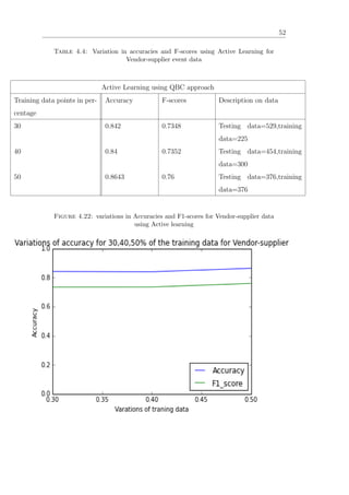
vendor-supplier test scores on a test data set of 225 data points. Similarly we
obtained failure results for job and acquistion events.
Table 4.40: Variation in test score for MFN with word embedding
Test score for MFN with word embedding on vendor-supplier dataset
Accuracy F-score Confusion matrix values
0.65 .39 True-negatives=140, True-positive = 13,
false-positives = 3, false-negatives = 69
4.7 Results obtained for Convolutional Neural
Networks
In convolutional neural network analysis is performed for each word initialized with
uniformly distributed random vector U[−1, 1] i.e. CNN-rand and CNN-word2vec
models which are as described in the section(3.5). Following displayed are the
results and analysis for both CNN models with 3-fold cross validation on the
whole data set.
4.7.1 Analysis for Vendor-Supplier Data using CNN-rand
and CNN-word2vec Model
Shape of the input matrix for vendor-supplier was 2515×300, which was maximum
sentence length × dimension of the corresponding word. The filter shapes used to
extract features were 3×300, 4×300 and 5×300. The dimension of the hidden
units was 100×2 dimension. The activation function used was RELU. Drop-out](https://image.slidesharecdn.com/3b17c844-45a8-4fef-a969-593e5d24747f-160105130418/85/Thesis-aligned-sc13m055-114-320.jpg)


![Bibliography
[1] Marujo, Luis, Wang Ling, Anatole Gershman, Jaime Carbonell, and Joo P.
Neto2 David Matos. Recognition of Named-Event Passages in News Articles.
In 24th International Conference on Computational Linguistics, pp.321-329.
2012.
[2] Marujo, Luis, Anatole Gershman, Jaime Carbonell, Robert Frederking, and
Joo P. Neto. Supervised topical key phrase extraction of news stories using
crowdsourcing, light filtering and co-reference normalization.In proceedings of
8th international conference on Language Resources and Evaluvation(LREC)
,pp.156-162. 2012.
[3] Su, Jiang, Jelber S. Shirab, and Stan Matwin. Large scale text classification
using semi-supervised multinomial naive bayes. In Proceedings of the 28th In-
ternational Conference on Machine Learning (ICML-11), pp. 97-104. 2011.
[4] Kim, Yoon. Convolutional Neural Networks for Sentence Classifica-
tion.Proceedings of the 2014 Conference on Empirical Methods in Natural
Language Processing (EMNLP), pp. 1746-1751. 2014.
[5] Nigam, Kamal, Andrew McCallum, and Tom Mitchell. Semi-supervised text
classification using EM. Semi-Supervised Learning,pp 33-56. 2006.
[6] Friedman, Jerome H.Greedy function approximation: a gradient boosting ma-
chine. Annals of statistics:pp 1189-1232. 2001.
[7] Freund, Yoav, and Robert E. Schapire. A desicion-theoretic generalization of
on-line learning and an application to boosting. In Computational learning
theory, pp. 23-37. Springer Berlin Heidelberg, 1995.
101](https://image.slidesharecdn.com/3b17c844-45a8-4fef-a969-593e5d24747f-160105130418/85/Thesis-aligned-sc13m055-124-320.jpg)
![102
[8] Breiman, Leo. Random forests. Machine learning 45, no. 1 (2001),pp. 5-32.
2001.
[9] Mikolov, Tomas, Kai Chen, Greg Corrado, and Jeffrey Dean. Efficient estima-
tion of word representations in vector space. arXiv preprint arXiv:1301.3781
(2013).
[10] Abe, N., and Mamitsuka, H. Query learning strategies using boosting and
bagging. Proceedings of 15th International Conferenec on Machine Learning
(ICML-98), pp. 1-10. 1998.
[11] Prem Melville and Raymond J. Mooney.Diverse Ensembles for Active
Learning.Proceedings of the 21st International Conference on Machine
Learning,(ICML-2004), pp. 584-591. 2004.
[12] Ramos, Juan.Using tf-idf to determine word relevance in document queries.
In Proceedings of the first instructional conference on machine learning. 2003.
[13] Collobert, J. Weston, L. Bottou, M. Karlen, K. Kavukcuglu, P. Kuksa. Natu-
ral Language Processing (Almost) from Scratch. Journal of Machine Learning
Research 12,pp. 2493-2537. 2011.
[14] Jenny Rose Finkel, Trond Grenager, and Christopher Manning. 2005. Incor-
porating Non-local Information into Information Extraction Systems by Gibbs
Sampling. Proceedings of the 43nd Annual Meeting of the Association for Com-
putational Linguistics (ACL 2005), pp. 363-370. 2005.
[15] Manning, Christopher D., Surdeanu, Mihai, Bauer, John, Finkel, Jenny,
Bethard, Steven J., and McClosky, David. 2014.The Stanford CoreNLP Nat-
ural Language Processing Toolkit. In Proceedings of 52nd Annual Meeting of
the Association for Computational Linguistics: System Demonstrations(ACL-
2014), pp. 55-60.2014.
[16] Hobbs, Jerry R.; Walker, Donald E.; Amsler, Robert A. (1982).Natural lan-
guage access to structured text Proceedings of the 9th conference on Compu-
tational linguistics 1. pp. 127-132.](https://image.slidesharecdn.com/3b17c844-45a8-4fef-a969-593e5d24747f-160105130418/85/Thesis-aligned-sc13m055-125-320.jpg)
![103
[17] Tjong Kim Sang, E. F., De Meulder, F. (2003, May). Introduction to the
CoNLL-2003 shared task: Language-independent named entity recognition. In
Proceedings of the seventh conference on Natural language learning at HLT-
NAACL 2003-Volume 4 (pp. 142-147). Association for Computational Linguis-
tics.
[18] Nadeau, D., Sekine, S. (2007).A survey of named entity recognition and clas-
sification. Lingvisticae Investigationes, 30(1) , pp 3-26, 2007.
[19] Soon, W. M., Ng, H. T., Lim, D. C. Y. (2001). A machine learning approach
to coreference resolution of noun phrases. Computational linguistics, 27(4) ,pp.
521-544.
[20] Pang, B., Lee, L. (2008).Opinion mining and sentiment analysis. Foundations
and trends in information retrieval,Volume 2 ,Issue 1-2, January 2008, pp. 1-
135 .
[21] Rowe, Ryan, German Creamer, Shlomo Hershkop, and Salvatore J. Stolfo.
Automated social hierarchy detection through email network analysis. In Pro-
ceedings of the 9th WebKDD and 1st SNA-KDD 2007 workshop on Web mining
and social network analysis, pp. 109-117. ACM, 2007.
[22] Liddy, E.D. 2001. Natural Language Processing. In Encyclopedia of Library
and Information Science, 2nd Ed. NY. Marcel Decker, Inc.
[23] Harris, Zellig S.Distributional structure.Word, Vol 10, 1954, pp. 146-162.
[24] Manning, C. D.; Raghavan, P.; Schutze, H. (2008). Scoring, term weighting,
and the vector space model. Introduction to Information Retrieval (PDF).pp.
52-100.
[25] Powers, David M W(2011).Evaluvation:From Precision, Recall and F-measure
to ROC, informedness, Markedness and Correlation.Journal of Machine Learn-
ing Technologies 2(1):37-63](https://image.slidesharecdn.com/3b17c844-45a8-4fef-a969-593e5d24747f-160105130418/85/Thesis-aligned-sc13m055-126-320.jpg)