The document outlines the author's preparation for coding interviews at Google, including a review of important data structures, algorithms, and problem domains. The author plans to thoroughly review arrays, trees, graphs, dynamic programming, recursion, sorting, strings, caching, game theory, computability, bitwise operators, math, concurrency, and system design. They will also practice solving problems involving arrays, strings, trees, graphs, divide-and-conquer, dynamic programming, and more. The single document the author intends to bring summarizes their background, projects, most difficult bugs, and other experiences that may be relevant questions during the interview.
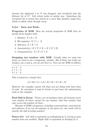
![B-Tree In computer science, a B-tree is a self-balancing tree data
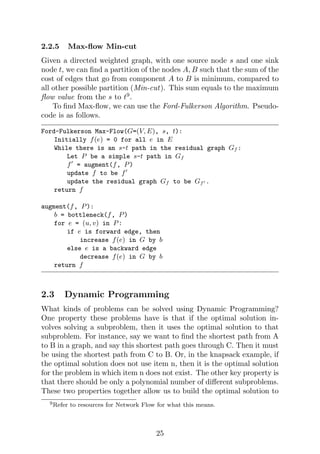
structure that keeps data sorted and allows searches, sequential access,
insertions, and deletions in logarithmic time. The B-tree is a general-
ization of a binary search tree in that a node can have more than two
children (Comer 1979, p. 123). For an interview, I doubt that we need to
know implementation details for a B-Tree. Know its motivation through.
Motivation: Self-balanced binary search tree (e.g. AVL tree) is slow
when the height of the tree reaches a certain limit such that manipulating
nodes require disk access. In fact, for a large dictionary, most of the data
is stored on disk. So we want a self-balancing tree that is even shallower
than AVL tree, to minimize the number of disk accesses, and exploit
disk block size.
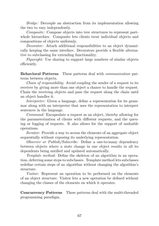
Binary Indexed Tree A binary indexed tree, also called a Fenwick
tree, is a data structure that can efficiently update elements and calculate
prefix sums in a table of numbers. I used it for the 2D Range sum
problem (3.8). See my implementation of 2D binary indexed tree there.
Motivation: Suppose we have an array arr with length n, we want
to (1) find the sum of first k elements, and (2) update the value of the
element arr[i], both in O(logn) time.
How it works4
: The core idea behind BIT is that every integer can
be written as the sum of power 2’s. Each node in a BIT stores the sum
of a range [i, j], and with all nodes combined, the BIT will cover the
entire range of the array. There needs to be a dummy root node, so the
size of BIT is n + 1. Here is how we build up the BIT for this array.
First, we initialize an array BIT with size n + 1 and all elements set
to 0. Then, we iterate through arr. For element i, we do an update for
the BIT array as follows:
1. We look at the node BIT[i+1]. We add arr[i] to it so
BIT[i+1]=BIT[i+1]+arr[i].
2. Now since we changed the range sum of a node, we have to update
the value of some other nodes. We can obtain the index n of the
next node with respect to node j for updating using the following
formula:
n=j+j&(-j).
4Watch YouTube video for decent explanation, by Tushar Roy: https://www.
youtube.com/watch?v=CWDQJGaN1gY&t=13s
15](https://image.slidesharecdn.com/codinginterviewpreparation-210311093651/85/Coding-interview-preparation-15-320.jpg)
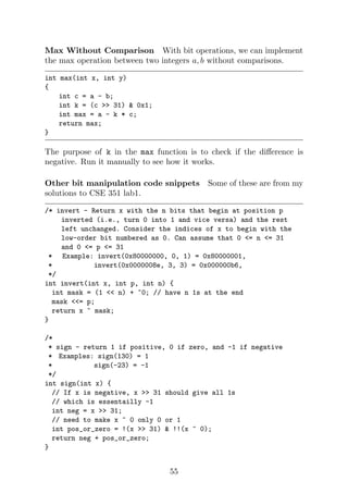
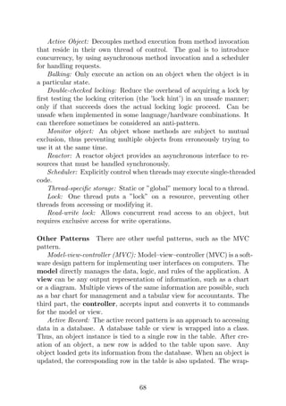
![We add the value arr[i] to each of the affected node, until the
computed index n is out of bound. The run time here is O(logn).
Here is how we use a BIT to compute the prefix sum of the first k
elements. Just like before, we find the BIT node with index k+1. We
add the value of that node to our sum. Then, traverse from the node
BIT[i+1] back to the root. Each time we go to the parent node of current
node, suppose BIT[j], we compute the index of that parent node p, by
p=j-j&(-j)
Then we add the value of the parent node to sum, until we reach the
root. Return sum as the result. This process is also O(logn) time. The
space of BIT is O(n).
2.1.16 Union-Find
A union-find data structure, also called a disjoin-set data structure, is a
data structure that maintains a set of disjoint subsets (e.g. components
of a graph). It supports two operations:
1. Find(u): Given element u, it will return the name of the set that
u is in. This can be used for checking if u and v are in the same
set. Optimal run time: O(logn).
2. Union(N1, N2): Given disjoint sets N1, N2, this operation will
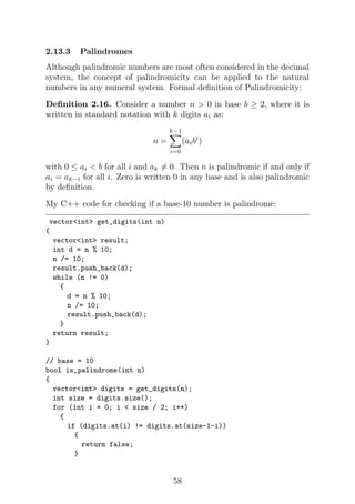
merge the two components into one set. Optimal run time O(1) if
we use pointers; if not, it is O(logn).
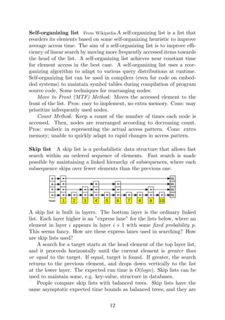
First, we will discuss an implementation using implicit list. Assume
that all objects can be labeled by numbers 1, 2, 3, · · · . Suppose we have
three disjoint sets as shown in the upper part of the following image.
Notice that the above representation is called an explicit list, because it
explicitly connects objects within a set together.
16](https://image.slidesharecdn.com/codinginterviewpreparation-210311093651/85/Coding-interview-preparation-16-320.jpg)
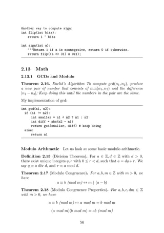
![As shown in the lower part of the image above, we can use a single
implicit list to represent the disjoint sets that can remember (1) pointers
to the canonical element (i.e. name) for a disjoint set, (2) the size of each
disjoint set. See appendix 5.3 for my Python implementation of Union-
Find, using implicit list.
When we union two sets, it is conceptually like joining two trees to-
gether, and the root of the tree is the canonical element of the set after
union. Path compression is basically the idea that we always join the
tree with smaller height into the one with greater height, i.e. the root of
the taller tree will be the root of the new tree after union. In my imple-
mentation, I used union-by-size instead of height, which can produce the
same result in run time analysis5
. The run time of union is determined
by the run time of find in this implementation. Analysis shows that
the upper bound of run time of find is the inverse Ackermann function,
which is even better than O(logn).
There is another implementation that uses tree that is also optimal
for union. In this case, the union-find data structure is a collection of
trees (forest), where each tree is a subset. The root of the tree is the
canonical element (i.e. name) of the disjoint set. It is essentially the
same idea as implicit list.
2.2 Trees and Graph algorithms
2.2.1 BFS and DFS
Pseudo-code BFS and DFS needs no introduction. Here is the pseudo-
code. The only difference here between BFS and DFS is that, for BFS,
we use queue as worklist, and for DFS, we use stack as worklist.
BFS/DFS(G=(V,E), s) {
worklist = [s]
seen = {s}
while worklist is not empty:
node = worklist.remove
{visit node}
for each neighbor u of node:
if u is not in visited:
queue.add(u)
seen.add(u)
}
5Discussed in CSE 332 slides, by Adam Blank: https://courses.cs.washington.
edu/courses/cse332/15au/lectures/union-find/union-find.pdf.
17](https://image.slidesharecdn.com/codinginterviewpreparation-210311093651/85/Coding-interview-preparation-17-320.jpg)
![There is another way to implement DFS using recursion (From MIT
6.006 lecture):
DFS(V , Adj):
parent = {}
for s in V :
if s is not in parent:
parent[s] = None
DFS-Visit(Adj, s, parent)
DFS-Visit(Adj, s, parent):
for v in Adj[s]:
if v is not in parent:
parent[v] = s
DFS-Visit(Adj, v, parent)
Obtain BFS/DFS layers BFS/DFS results in BFS/DFS-tree, which
has layers L1, L2, · · · . Each layer is a set of vertices. BFS layers are really
useful for problems such as determining if the graph is two-colorable.
DFS layers are useful too (application?)
BFS/DFS(G=(V,E), s) {
worklist = [s]
seen = {s}
layers = {s:0}
while worklist is not empty:
node = worklist.remove
{visit node}
for each neighbor u of node:
if u is not in visited:
queue.add(u)
seen.add(u)
layers.put(u, layers[node]+1)
Go through keys in layers and obtain the set of nodes for
each layer.
}
Now we will look at some BFS/DFS Tree Theorems.
Theorem 2.1 (BFS). For each j ≥ 1, layer Lj produced by BFS starting
from node s consists of all nodes at distance exactly j from s.
Theorem 2.2 (BFS). There is a path from s to t if and only if t appears
18](https://image.slidesharecdn.com/codinginterviewpreparation-210311093651/85/Coding-interview-preparation-18-320.jpg)
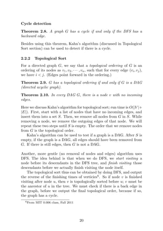
![2.2.3 Paths
Obtain BFS/DFS path from s to t When we have an unweighted
graph, we can find a path from s to t simply by BFS or DFS. BFS gives
the shortest path in this case. It is straightforward if we have a map
that can tell the parent of each node in the tree.
BFS/DFS(G=(V,E), s, t):
worklist = [s]
seen = {s}
parent = {s:None}
while worklist is not empty:
node = worklist.remove
if node == t:
return Get-Path(s, t, parent)
for each neighbor u of node:
if u is not in visited:
queue.add(u)
seen.add(u)
parent[u] = node
return NO PATH
Get-Path(s, t, parent):
v = t
path = {t}
while v != s:
v = parent[v]
path.add(v)
return path
Dijkstra’s Algorithm This algorithm is for finding the shortest path
from s to t on a graph with nonnegative weights. When choosing the
node v, if we use Fibonacci Heap to store the edges, then the run time
can be O(|E| + |V |log|V |).
Dijkstra’s-Algorithm(G=(V,E), s, t):
S = {}; d[s] = 0; d[v] = infinity for v != s
prev[s] = None
While S != V
Choose v in V-S with minimum d[v]
Add v to S
For each w in the neighborhood of v
if d[v] + c(v,w) < d[w]:
21](https://image.slidesharecdn.com/codinginterviewpreparation-210311093651/85/Coding-interview-preparation-21-320.jpg)
![d[w] = d[v] + c(v,w)
prev[w] = v
return d, prev
This algorithm works by expanding a set S starting from s, within which
we have nodes such that the shortest paths from s to these nodes are
known. The step that chooses v from the set difference between V and
S with minumum d[v] is equivalent as choosing the edge with minimum
weight that goes from S to V − S.
Bellman-Ford Algorithm This algorithm works for graph that has
negative edge weights, but no negative cycles. Its run time is O(|V ||E|).
Bellman-Ford(G=(V,E), s, t):
d[s] = 0; d[v] = infinity for v != s
prev[s] = None
for i = 1 to |V|-1:
for each edge (u, v) with weight w in E:
if d[u] + w < d[v]:
d[v] = d[u] + w
prev[v] = u
return d, prev
A* Algorithm Proposed by P.Hart et. al., this algorithm is an ex-
tension of Dijkstra’s algorithm. It achieves better performance by using
heuristics to guide its search. A* algorithm finds the path that mini-
mizes
f(n) = g(n) + h(n)
where n is the last node on the path, g(n) is the cost of the path from
the start node to n, and h(n) is a heuristic that estimates the cost of
the cheapest path from n to the goal. The heuristic must be admissible,
i.e. it never overestimates the actual cost to get to the goal. Below is
my implementation with Python, when I took the CSE 473 (Artificial
Intelligence) class:
def aStarSearch(problem, heuristic=nullHeuristic):
"""Search the node that has the lowest combined cost and
heuristic first."""
startState = problem.getStartState()
visitedStates = set({})
worklist = util.PriorityQueue()
22](https://image.slidesharecdn.com/codinginterviewpreparation-210311093651/85/Coding-interview-preparation-22-320.jpg)
![# First tuple means (state, path_to_state, cost_of_path)
worklist.push((startState, [], 0),
0 + heuristic(startState, problem))
while not worklist.isEmpty():
state, actions, pathCost = worklist.pop()
if state in visitedStates:
continue
if problem.isGoalState(state):
return actions
successors = problem.getSuccessors(state)
for stepInfo in successors:
sucState, action, stepCost = stepInfo
sucPathCost = pathCost + stepCost
worklist.push((sucState, actions + [action],
sucPathCost),
sucPathCost + heuristic(sucState,
problem))
# mark the current state as visited
visitedStates.add(state)
# Not able to get there
return None
All-pairs shortest paths This problem concerns finding all paths
between every pair of vertices. A well-known algorithm for this is the
Floyd-Warshall’s algorithm, which runs in O(|V |3
) time. It works for
graphs with positive or negative weights, with no negative cycles. Its
run time is impressive, considering the fact that there may be up to
Ω(|V |2
) edges in a graph. This is a dynamic programming algorithm.
The algorithm considers a function shortestPath(i, j, k) which
finds the shortest path from i to j with only vertices {v1, v2, · · · , vk} ⊂
V . Given that for every pair of nodes i and j, we know the output
of shortestPath(i, j, k), our goal is to figure out the output of
shortestPath(i, j, k+1) for every such pair. When we have a new
vertex, vk+1, either the path from vi to vj goes through vk+1, or not.
This brings us to the core of Floyd-Warshall’s algorithm:
shortestPath(i, j, k+1) = min(shortestPath(i, j, k),
shortestPath(i, k+1, k) + shortestPath(k+1, j, k))
23](https://image.slidesharecdn.com/codinginterviewpreparation-210311093651/85/Coding-interview-preparation-23-320.jpg)
![the final problem from optimal solutions to subproblems10
.
2.3.1 One example problem involving 2-D table
Problem: Given a string x consisting of 0s and 1s, we write xk
to denote k
copies of x concatenated together. We say that a string x0
is a repetition
of x if it is a prefix of xk
for some number k. So x0
= 10110110110 is a
repetition of x = 101.
We say that a string s is an interleaving of x and y if its symbols
can be partitioned into two (not necessarily contiguous) subsequences s0
and s00
, so that s0
is a repetition of x, and s00
is a repitition of y. For
example, if x = 101, and y = 00, then s = 100010101 is an interleaving
of x and y, since characters 1,2,5,7,8,9 form 101101 – a repetition of x –
and the remaining characters 3,4,6 form 000, a repitition of y.
Give an efficient algorithm that takes strings s, x, y, and decide if s
is an interleaving of x and y11
.
My Solution Our Opt table will look like this.(Consider / as an empty
character, which means including / in a substring is as if we included
nothing). Assume that the length of string s is l.
/ x0
1 · · · x0
l
/ True
y0
1
· · ·
y0
l
The value of each cell is either True or False. Strictly,
Opt[xi, yj] = True if and only if
Opt[xi, yj−1] = True AND s[i + j] = y0
[j] OR,
Opt[xi−1, yj] = True AND s[i + j] = x0
[i].
(If x0
[i] = / or y0
[j] = /, then we treat s[i+j] = x0
[i and s[i+j] = y0
[j]
to be True.
We can think of a cell being True as there is an interleaving of i
characters of x0
and j characters of y0
that makes up the first i + j
characters of string s.
If we filled out this table, we can return True if for some i and j such
that i is a multiple of |x| AND j is a multiple of |j| AND i + j = l AND
10Cited from CMU class lecture note: https://www.cs.cmu.edu/~avrim/451f09/
lectures/lect1001.pdf
11This problem is from Algorithm Design, by Kleinberg, Tardos, pp.329 19.
26](https://image.slidesharecdn.com/codinginterviewpreparation-210311093651/85/Coding-interview-preparation-26-320.jpg)
![Opt[i, j] = True. This is precisely saying that we return True if s can
be composed by interleaving some repetition of x and y.
So first, our job now is to fill up this table. We can traverse j from 1
to l (traverse each row). And inside each iteration, we traverse i from 1
to l. Inside each iteration of this nested loop, we set the value of Opt[i,
j] according to the rule described above.
Then, we can come up with i and j by fixing i and increment j by
|y| until i + j > l (*). Then, we increment i by |x|. Then, we repeat the
previous step (*), and stop when i + j > l. We check if i + j = l inside
each iteration, and if so, we check if Opt[i,j]=True. If yes, we return
True. If we don’t return True, we return False at the end.
2.3.2 Well-known problems solved by DP
Longest Common Subsequence Find the longest subsequence com-
mon to all sequences in a set S of sequences. Unlike substrings, sub-
sequences are not required to occupy consecutive positions within the
original sequences.
Let us look at the case where there are only two sequences x, y
in S. For example, x is 14426, and y is 2134. The longest common
subsequence of x and y is then 14. Define Opt[i, j] to be the longest
common subsequence for subsring x[0 : i] and y[0 : j]. We have the
following update formula:
Opt =
∅ if i = 0, j = 0
Opt[i − 1, j − 1] ∪ xi if x[i] = y[j]
max(Opt[i − 1, j], Opt[i, j − 1]) if x[i] 6= y[j]
Similar problems: longest common substring, longest increasing subsequence).
Now, let us discuss the Levenshtein distance problem. The Lev-
enshtein distance measures the difference between two sequences, i.e.
the fewest number of operations (edit, delete, add) to change from one
sequence to another. The definition of Levenshtein distance is itself a
dynamic programming solution to find the edit distance, as follows (from
Wikipedia):
Definition 2.1. The Levenshtein distance between two strings a, b (of
length |a| and |b| respectively) is given by leva,b(|a|, |b|) where
leva,b(i, j) =
max(i, j) if min(i, j) = 0,
min
leva,b(i − 1, j) + 1
leva,b(i, j − 1) + 1
leva,b(i − 1, j − 1) + 1(ai6=bj )
otherwise.
27](https://image.slidesharecdn.com/codinginterviewpreparation-210311093651/85/Coding-interview-preparation-27-320.jpg)
![where 1(ai6=bj ) is the indicator function that equals to 1 if ai 6= bj, and
leva,b(i, j) is the distance between the first i characters of a and the first
j characters of b.
The Knapsack Problem Given a set of items S, with size n, each
item ai with a weight wi and a value vi, determine the number of each
item to include in a collection so that the total weight is less than or
equal to a given limit K and the total value is as large as possible.
Define Opt[i, k] to be the optimal subset of items from a1, · · · , ai such
that the total weight does not exceed k. Our final result will then be
given by Opt[n, K]. For an item ai, either it is included into the subset,
or not. If not, that means the total weight of the subset with ai added
exceeds k. Therefore we have:
Opt[i, k] =
∅ if k=0,
Opt[i − 1, k] if adding wi exceeds k,
max(Opt[i − 1, k],
Opt[i − 1, k − wi] + vi) otherwise
Similar problems: subset sum.
Matrix Chain Multiplication Given a sequence of matrices A1A2 · · · An,
the goal is to find the most efficient way to multiply these matrices. The
problem is not actually to perform the multiplications, but merely to
decide the sequence of the matrix multiplications involved.
Here are many options because matrix multiplication is associative.
In other words, no matter how the product is parenthesized, the result
obtained will remain the same. For example, for four matrices A, B, C,
and D, we would have:
((AB)C)D = ((A(BC))D) = (AB)(CD) = A((BC)D) = A(B(CD))
However, the order in which the product is parenthesized affects the
number of simple arithmetic operations needed to compute the product,
or the efficiency. For example, if A is a 10×30 matrix, B is a 30×5
matrix, and C is a 5 × 60 matrix, then computing (AB)C needs
(10 × 30 × 5) + (10 × 5 × 60) = 1500 + 3000 = 4500
operations, while computing A(BC) needs
(30 × 5 × 60) + (10 × 30 × 60) = 9000 + 18000 = 27000
28](https://image.slidesharecdn.com/codinginterviewpreparation-210311093651/85/Coding-interview-preparation-28-320.jpg)
![operations. The first parenthesization is obviously more preferable.
Given n matrices, the total number of ways to parenthesize them is
P(n) = Ω(4n
/n3/2
), so brute force is impractical12
.
We use dynamic programming. First, we characterize the structure
of an optimal solution. We claim that one possible structure is the
following:
((A1:i)(Ai+1:n)) (1)
where Ai:j means matrix multiplication of AiAi+1 · · · Aj. In order for
the above to be optimal, the parenthesization for A1:i and Ai+1:n must
also be optimal. Therefore, we can recursively break down the problem,
till we only have one matrix. A subproblem is of the form Ai:j, with 1 ≤
i, j ≤ n, which means there are O(n2
) unique subproblems (counting).
Let Opt[i, j] be the cost of computing Ai:j. If the final multiplication
of Ai:j is Ai:j = Ai:kAk+1,j, assuming that Ai:k is pi−1 × pk, and Ak+1:j
is pk × pj, then for i < j,
Opt[i, j] = Opt[i, k] + Opt[k + 1, j] + pi−1pkpj
This is because by definition of Opt, we need Opt[i, k] to compute Ai:k,
and Opt[k + 1 : j] to compute Ak+1:j, and pi−1pkpj to compute the
multiplication of A1:k and Ak+1:j. For i = j, Opt[i, j] = 0. Since we
need to check all values of i, j pair, i.e. the parenthesization shown in
(1), the run time is O(n3
).
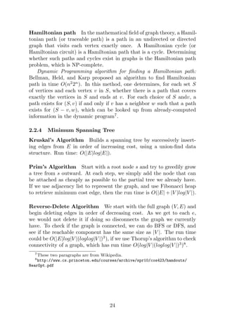
2.3.3 Top-down dynamic programming
So far, we are able to come up with an equation for the Opt table/array
in the example problems above. This is called bottom-up approach.
However, for some problems, it is not easy to determine such equation.
In this case, we can use memoization and top-down approach, usually
involving recursion. The top-down approach basically leads to the same
algorithm as bottom-up, but the perspective is different. According to
a lecture note of CMU algorithms class:
Basic Idea: Suppose you have a recursive algorithm for some
problem that gives you a really bad recurrence like T(n) =
2T(n − 1) + n. However, suppose that many of the subprob-
lems you reach as you go down the recursion tree are the same.
Then you can hope to get a big savings if you store your com-
putations so that you only compute each different subproblem
12Columbia class slides: http://www.columbia.edu/~cs2035/courses/csor4231.
F11/matrix-chain.pdf.
29](https://image.slidesharecdn.com/codinginterviewpreparation-210311093651/85/Coding-interview-preparation-29-320.jpg)
![once. You can store these solutions in an array or hash table.
This view of Dynamic Programming is often called memoizing.
For example, the longest common subsequence (LCS) problem can be
solved with this top-down approach. Here is the pseudo-code, from the
CMU lecture note.
LCS(S,n,T,m)
{
if (n==0 || m==0)
return 0;
if (arr[n][m] != unknown)
return arr[n][m]; // memoization (use)
if (S[n] == T[m])
result = 1 + LCS(S,n-1,T,m-1);
else
result = max( LCS(S,n-1,T,m), LCS(S,n,T,m-1) );
arr[n][m] = result; // memoization (store)
return result;
}
If we compare the above code with the bottom-up formula for LCS, we
realize that they are just using the same algorithm, with same cases. The
idea that both approaches share is that, we only care about computing
the value for a particular subproblem.
2.4 Recursive algorithms
2.4.1 Divide and Conquer
The matrix chain multiplication problem discussed previously can be
solved, using top-down approach, with recursion, and the idea there
is basically divide and conquer – break up the big chain into smaller
chains, until i = j (Opt[i, j]=0). Divide and conquer (D&C) works by
recursively breaking down a problem into two or more sub-problems of
the same or related type, until these problems are simple enough to be
solved directly13
. For some problems, we can use memoization technique
to optimize the run time.
Now, let us look at two well-known problems solvable by divide-and-
conquer algorithms.
13From Wikipedia.
30](https://image.slidesharecdn.com/codinginterviewpreparation-210311093651/85/Coding-interview-preparation-30-320.jpg)
![Binary Search This search algorithm runs in O(logn) time. It works
by comparing the target element with the middle element of the array,
and narrow the search to half of the array, until the middle element is
exactly the target element, or until the remaining array has only one
element. Binary search is naturally a divide-and-conquer algorithm.
Binary-Search-Recursive(arr, target, lo, hi):
# lo inclusive, hi exclusive.
if hi <= lo:
return NOT FOUND
mid = lo + (hi-lo)/2
if arr[mid] == target:
return mid
else if arr[mid] > target
return Binary-Search-Recursive(arr, target, mid+1, hi)
else:
return Binary-Search-Recursive(arr, target, lo, mid)
Binary-Search-Iterative(arr, target):
lo = 0
hi = arr.length
while lo < hi:
mid = lo + (hi-lo)/2
if arr[mid] == target:
return mid
else if arr[mid] > target:
lo = mid + 1
else:
hi = mid
return NOT FOUND
Implement the square root function: To implement the square root
function programmatically, with integer return value, we can use binary
search. Given number n, we know that the square root of n must lie
between 0 and n/2. Then, we can basically treat all integers in [0, n/2]
as an array, and do binary search. We terminate only when lo equals
to hi.
Closest Pair of Points Given n points in metric space, e.g. plane,
find a pair of points with the smallest distance between them. A divide-
and-conquer algorithm is as follows (from Wikipedia):
1. Sort points according to their x-coordinates.
31](https://image.slidesharecdn.com/codinginterviewpreparation-210311093651/85/Coding-interview-preparation-31-320.jpg)
![2. Split the set of points into two equal-sized subsets by a vertical
line x = xsplit.
3. Solve the problem recursively in the left and right subsets. This
yields the left-side and right-side minimum distances dLmin and
dRmin, respectively.
4. Find the minimal distance dLRmin among the set of pairs of points
in which one point lies on the left of the dividing vertical and the
other point lies to the right.
5. The final answer is the minimum among dLmin, dRmin, and dLRmin.
The recurrence of this algorithm is T(n) = 2T(n/2) + O(n), where O(n)
is the time needed for step 4. This recurrence to O(nlogn). Why can
step 4 be completed in linear time? How? Suppose from step 3, we know
the current minimum distance is δ. For step 4, we first pick the points
with x-coordinates that are within [xsplit − δ, xsplit + δ], call this the
boundary zone. Suppose we have p1, · · · , pm inside the boundary zone.
Then, we have the following magical theorem.
Theorem 2.11. If dist(pi, pj) < δ, then j − i ≤ 15.
With this, we can write the pseudo-code for this algorithm14
:
Closest-Pair(P):
if |P| == 2:
return dist(P[0], P[1])
L, R = SplitPointsByHalf(P)
dL = Closest-Pair(L)
dR = Closest-Pair(R)
dLR = min(dL, dR)
S = BoundaryZonePoints(L, R, dLR)
for i = 1, ..., |S|:
for j = 1, ..., 15:
dLR = min(dist(S[i], S[j]), d)
return dLR
Obviously, there are other classic divide-and-conquer algorithms to solve
problems such as the convex hull (two-finger algorithm), and the median
of medians algorithm (groups of five). As the writer, I have read those
14Cited from CMU lecture slides, with modification https://www.cs.cmu.edu/
~ckingsf/bioinfo-lectures/closepoints.pdf
32](https://image.slidesharecdn.com/codinginterviewpreparation-210311093651/85/Coding-interview-preparation-32-320.jpg)
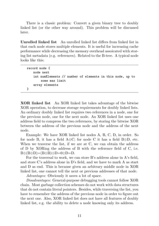
![rithm produces optimal result for 0 <= j <= k. Thus, the result
produced by the algorithm for n = k + 1 matches the optimal in
case (b), which is to NOT call status check any more.
Conclusion From the above proof of base case and induction
step, by Strong Induction, we have shown that our algorithm
works for integer n >= 0.
Indeed, induction is how you formally prove that a greedy rule works
correctly.
Justification for run time: The above algorithm is efficient. We first
construct a heap of processes, which takes O(nlogn) time. Then we loop
until we remove all items inside the heap, which is O(nlogn) time. Since
we do not add any process back into the heap after we removed it, the
algorithm will terminate when the heap is empty. Besides, any other
operations in the algorithm is O(1). Therefore, combined, our algorithm
has an efficient runtime of O(nlogn) + O(nlogn) = O(nlogn).
2.6 Sorting
2.6.1 Merge sort
Merge sort is a divide-and-conquer, stable sorting algorithm. Worst case
O(nlogn); Worst space O(n). Here is a pseudo-code for non-in-place
merge sort. An in-place merge sort is possible.
Mergesort(arr):
if arr.length == 1:
return arr
l = Mergesort(arr[0:mid])
r = Mergesort(arr[mid:length])
return merge(l, r)
2.6.2 Quicksort
Quicksort is a divide-and-conquer, unstable sorting algorithm. Average
run time O(nlogn); Worst case run time O(n2
); Worst case auxiliary
space18
O(logn) with good implementation. (Naive implementation is
O(n) space still.) Quicksort is fast if all comparisons are done with
constant-time memory access (assumption). People have argued which
sort is the best. Here is an answer from Stackoverflow, by user11318:
18Auxiliary Space is the extra space or temporary space used by an algorithm.
From GeeksForGeeks.
36](https://image.slidesharecdn.com/codinginterviewpreparation-210311093651/85/Coding-interview-preparation-36-320.jpg)
![... However if your data structure is big enough to live on disk,
then quicksort gets killed by the fact that your average disk does
something like 200 random seeks per second. But that same disk
has no trouble reading or writing megabytes per second of data
sequentially. Which is exactly what merge sort does.
Therefore if data has to be sorted on disk, you really,
really want to use some variation on merge sort. (Gen-
erally you quicksort sublists, then start merging them together
above some size threshold.) ...
Here is the pseudo-code:
Quicksort(arr, lo, hi):
# lo inclusive, hi exclusive
if hi <= lo:
return
pivot = ChoosePivot(arr, lo, hi)
p = Partition(arr, lo, hi, pivot)
Quicksort(arr, lo, p)
Quicksort(arr, p, hi)
Partition(arr, lo, hi, pivot):
# lo inclusive, hi exclusive
i = lo, j = hi
while i < j:
if arr[i] < pivot:
i += 1
else:
swap(arr, i, j-1)
j -= 1
return i # sorted position of pivot
A nice strategy for choosing pivot is to just choose randomly. Another
good way is to choose the median value from the first, last and middle
element of the array.
2.6.3 Bucket sort
Bucket sort in some cases can achieve O(n) run time. But it is unstable
(worst case O(n2
). It works by distributing the elements of an array
into a number of buckets. Each bucket is then sorted individually, either
using a different sorting algorithm, or by recursively applying the bucket
sorting algorithm.
37](https://image.slidesharecdn.com/codinginterviewpreparation-210311093651/85/Coding-interview-preparation-37-320.jpg)
![if hi <= lo:
return arr[lo]
pivot = ChoosePivot(arr, lo, hi)
p = Partition(arr, lo, hi, pivot)
if p == k:
return arr[k]
else if p > k:
return Quickselect(arr, k, lo, p)
else:
return Quickselect(arr, k-p, p, hi)
The (expected) recurrence for the above psuedo-code is T(n) = T(n/2)+
O(n). When solved, it gives O(n) run time. For the worst case, which
is also due to bad pivot selection, the run time is O(n2
).
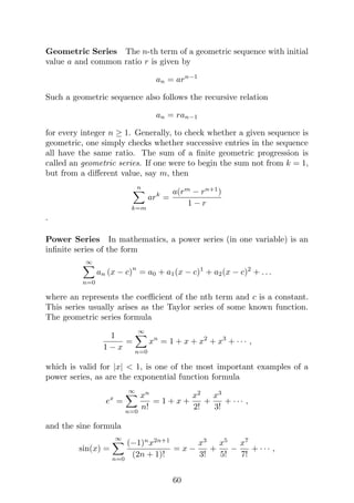
2.8 String
2.8.1 Regular expressions
Regular expression needs no introduction. In interviews, the interviewer
may ask you to implement a regular expression matcher for a subset of
regular expression symbols. Similar problems could be asking you to
implement a program that can recognize a particular string pattern.
Here is a regex matcher written by Brian Kernighan and Rob Pike
in their book The Practice of Programming21
.
/* match: search for regexp anywhere in text */
int match(char *regexp, char *text)
{
if (regexp[0] == ’^’)
return matchhere(regexp+1, text);
do { /* must look even if string is empty */
if (matchhere(regexp, text))
return 1;
} while (*text++ != ’0’);
return 0;
}
/* matchhere: search for regexp at beginning of text */
int matchhere(char *regexp, char *text)
{
21Discussed here http://www.cs.princeton.edu/courses/archive/spr09/
cos333/beautiful.html
39](https://image.slidesharecdn.com/codinginterviewpreparation-210311093651/85/Coding-interview-preparation-39-320.jpg)
![if (regexp[0] == ’0’)
return 1;
if (regexp[1] == ’*’)
return matchstar(regexp[0], regexp+2, text);
if (regexp[0] == ’#’ && regexp[1] == ’0’)
/* # means dollar sign here! */
return *text == ’0’;
if (*text!=’0’ && (regexp[0]==’.’ || regexp[0]==*text))
return matchhere(regexp+1, text+1);
return 0;
}
/* matchstar: search for c*regexp at beginning of text */
int matchstar(int c, char *regexp, char *text)
{
do { /* a * matches zero or more instances */
if (matchhere(regexp, text))
return 1;
} while (*text != ’0’ && (*text++ == c || c == ’.’));
return 0;
}
2.8.2 Knuth-Morris-Pratt (KMP) Algorithm
The KMP algorithm is used for the string matching problem.
Find the index that a pattern P with length m occurs (if ever) in
a string W with length n.
The naive algorithm to solve this problem takes O(nm) time, which does
not utilize any information when a matching failed. The key of KMP is
that it uses it and achieves run time of O(n + m). It is a complicated
algorithm, and let me explain it now. See the appendix 5.2 for my
Python implementation, based on the ideas below.
Building prefix table (π table) The first thing that KMP does is to
preprocess the pattern P and create a π table. π[i] is the largest integer
smaller than i such that P0 · · · Pπ[i] is a suffix of P0 · · · Pi. Consider the
following example:
i 0 1 2 3 4 5 6 7
Pi a b a b c a b a
π[i] -1 -1 0 1 -1 0 1 2
40](https://image.slidesharecdn.com/codinginterviewpreparation-210311093651/85/Coding-interview-preparation-40-320.jpg)
![When we are filling π[i], we focus on the substring P0 · · · Pi, and see if
there is a prefix equal to the suffix in that substring. π[0], π[1], π[4] are
−1, meaning that there is no prefix equal to suffix in the corresponding
substring. For example, for π[4], the substring of concern is ababc, and
there is no valid index value for π[4] to be set. π[7] = 2, because the
substring P0 · · · P7 is ababcaba, and the prefix P0 · · · P2, aba, is a suffix
of that substring.
Below is a pseudo-code for constructing a π table. The idea behind
the pseudo-code is captured by two observations:
1. If P0 · · · Pπ[i] is a suffix for P0 · · · Pi, then P0 · · · Pπ[i]−1 is a suffix
for P0 · · · Pi−1 as well.
2. If P0 · · · Pπ[i] is a suffix for P0 · · · Pi, then so does P0 · · · Pπ[π[i]], and
so does P0 · · · Pπ[π[π[i]]], etc., a recursion of the π values.
So we can use two pointers i, j, and we are always looking at if the
prefix P0 · · · Pj−1 is a suffix for the substring P0 · · · Pi−1. So pointer i
moves quicker than pointer j. In fact i moves up by 1 every time we are
done with a comparison between Pi and Pj, and j moves up by 1 when
Pi = Pj (observation 1). At this time (Pi = Pj), we set π[i] = j. If
Pi 6= Pj, we will move j back to π[j − 1] + 1 (+1 because π[i] is -1 when
there is no matching prefix.) This guarantees that the prefix P0 · · · Pj−1
is the longest suffix for the substring P0 · · · Pi−1. We need to initialize
π[−1] = −1 and π[0] = −1.
Construct-π-Table(P):
j = 0, i = 1
while i < |P|:
if Pi = Pj:
π[i] = j
i += 1, j += 1
else:
if j > 0:
j = max(0, π[j-1]+1)
else:
π[i] = -1
i += 1
Pattern Matching Once we have the π table, we can skip characters
when comparing the pattern P and the string W. Consider P and W to
41](https://image.slidesharecdn.com/codinginterviewpreparation-210311093651/85/Coding-interview-preparation-41-320.jpg)
![be the following, as an example. (P is the same as the above example.)
W = abccababababcaababcaba, P = ababcaba
Based on the way we construct the π table above, we have the following
rules when doing the matching. Assume the matched substring (i.e. the
substring of P before the first mismatch, starting at W[k], has length d.
1. If d = |P|, we found a match. Return k.
2. Else, if d > 0, and π[d − 1] = −1, then the next comparison starts
at W[k + d].
3. Else, if d > 0, and π[d − 1] 6= −1, then the next comparison starts
at. W[k + d − π[d − 1] − 1].Note: we don’t need the −1 here if π table is
1-based index. See Stanford slides.
4. Else, if the matched substring, starting at index k, has length 0,
then the next match starts at k + 1.
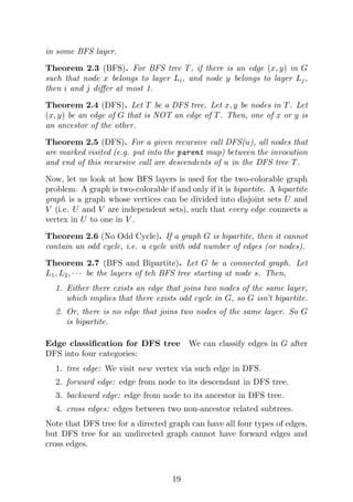
2.8.3 Suffix/Prefix Tree
See Trie 2.1.15. If we have a text of size T, and a small pattern of size
P, and we are interested to know if P occurs in T, then we can achieve
O(P) time and O(T) space by building a suffix tree of the text T. A
suffix tree is a compressed trie containing all the suffixes of the given text
as their keys and positions in the text as their values. Suffix trees allow
particularly fast implementations of many important string operations
(Wikipedia). The construction of such a tree for the string T takes time
and space linear in the length of T. Here is an example of a suffix tree,
for T = ”banana$”. (The $ sign is for marking the end of a string.)
42](https://image.slidesharecdn.com/codinginterviewpreparation-210311093651/85/Coding-interview-preparation-42-320.jpg)
![• A set of states s ∈ S,
• A set of actions a ∈ A,
• A transition function T(s, as0
) for the probability of transition from
s to s0
with action a,
• A reward function R(s, as0
),
• A start state,
• (maybe) a terminal state.
The world for MDP is usually a grid world, where some grids have pos-
itive reward, and some have negative reward. The goal of solving an
MDP is to figure out an optimal policy π∗
(s), the optimal action for
state s, so that the agent can take actions according to the policy in or-
der to gain the highest amount of reward possible. There are two ways to
solve MDP discussed in the undergraduate level AI class: value (utility)
iteration and policy iteration. I will just put some formulas here. For
most of the time, understanding them is straightforward and sufficient.
Definition 2.4. The utility of a state is V ∗
(s), the expected utility
starting in s and acting optimally.
Definition 2.5. The utility of a q-state25
is Q∗
(s, a), the expected util-
ity starting by taking action a in state s, and act optimally afterwards.
Using the above definition, we have the following recursive definition
of utilities. The γ value is a discount, from 0 to 1, which can let the
model prefer sooner reward, and help the algorithm converge. Note max
is different from argmax.
V ∗
(s) = max
a
Q∗
(s, a)
Q∗
(s, a) =
X
s0
T(s, a, s0
)[R(s, a, s0
) + γV ∗
(s0
)]
V ∗
(s) = max
a
X
s0
T(s, a, s0
)[R(s, a, s0
) + γV ∗
(s0
)]
Value Iteration: Start with V0(s) = 0 for all s ∈ S. Then, we update
Vk+1 iteratively using the following (almost trivial) update rule, until
convergence. Complexity of each iteration: O(S2
A).
Vk+1(s) ← max
a
X
s0
T(s, a, s0
)[R(s, a, s0
) + γVk(s0
)]
25The naming, q-state, from my understanding, means quasi-state, which is seem-
ingly a state, but not really.
47](https://image.slidesharecdn.com/codinginterviewpreparation-210311093651/85/Coding-interview-preparation-47-320.jpg)
![Policy Iteration: Start with an arbitrary policy π0, then iteratively
evaluate and improve the current policy until policy converges. This is
better than value iteration in that policy usually converges long before
value converges, and the run time for value iteration is not desirable.
V πi
k+1 ←
X
s0
T(s, πi(s), s0
)[R(s, πi(s), s0
) + γVk(s0
)πi
]
πi+1(s) = argmax
a
X
s0
T(s, a, s0
)[R(s, a, s0
] + γV πi
(s0
)]
2.10.3 Hidden Markov Models
A Hidden Markov Model looks like this:
A state is a value of a variable Xi. For example, if Xi is a random
variable meaning ”it rains on day i”, then the value of Xi can be True
or False. If X1 = t, then we have a state X1 which means it rains on
day 1.
An HMM is defined by an initial distribution P(X1), transitions
P(Xt|Xt−1), and emissions P(Et|Xt). The value of an emission vari-
able represents an observation, e.g. sensor readings.
We are interested to know P(Xt|e1:t), which is the distribution of Xt
given all of the observations to date. We can obtain the joint distribution
of xt ∈ Xt and all current observations.
P(xt, e1, · · · , et) = P(et|xt)
X
xt−1
P(xt|xt−1)P(xt−1, e1, · · · , et−1)
Then, we normalize all entries in P(Xt, e1, · · · , et) to the desired current
belief, B(Xt), by the definition of conditional probability.
B(Xt) = P(Xt|e1:t) = P(Xt, e1, · · · , et)/
X
xt
P(xt, e1, · · · , et)
48](https://image.slidesharecdn.com/codinginterviewpreparation-210311093651/85/Coding-interview-preparation-48-320.jpg)
![}
return true;
}
2.13.4 Combination and Permutation
Combination n choose k is defined as follows:
C(n, k) =
n
k
=
n(n − 1) · · · (n − k + 1)
k(k − 1) · · · 1
One property of combination:
n
k
=
n
n − k
Permutation n choose k where order matters can be expressed as
follows:
P(n, k) = n · (n − 1) · (n − 2) · · · (n − k + 1)
| {z }
k factors
=
n!
(n − k)!
C(n, k) =
P(n, k)
P(k, k)
=
P(n, k)
k!
=
n!
(n − k)!k!
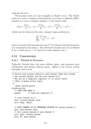
2.13.5 Series
The following description is from Wikipedia.
Arithmetic Series If the initial term of an arithmetic progression is
a1 and the common difference of successive members is d, then the nth
term of the sequence an is given by:
an = a1 + (n − 1)d
and in general
an = am + (n − m)d
A finite portion of an arithmetic progression is called a finite arithmetic
progression and sometimes just called an arithmetic progression. The
sum of a finite arithmetic progression is called an arithmetic series,
Sn =
n(a1 + an)
2
=
n
2
[2a1 + (n − 1)d]
59](https://image.slidesharecdn.com/codinginterviewpreparation-210311093651/85/Coding-interview-preparation-59-320.jpg)

![3 Flagship Problems
It turns out that I do not have a lot of time to complete many problems
and record the solutions here. I will include the description several im-
portant problems, and solve them after I print this out. I will update the
solutions hopefully eventually. Refer to 3.9 for these unsolved problems.
3.1 Arrays
Missing Ranges (Source. Leetcode 163) Given a sorted integer array
where the range of elements are in the inclusive range [lower, upper],
return its missing ranges.
For example, given [0, 1, 3, 50, 75], lower = 0 and upper =
99, return [2, 4-49, 51-74, 76-99].
My code:
class Solution(object):
def __getRange(self, a, b):
if b - a 1:
if b - a == 2:
return str(a+1)
else:
return str(a+1) + - + str(b-1)
else:
return None
def findMissingRanges(self, nums, lower, upper):
result = []
upper += 1
lower -= 1
lastOne = lower
if len(nums) 0:
lastOne = nums[len(nums)-1]
for i, n in enumerate(nums):
rg = None
if i == 0:
# First number
rg = self.__getRange(lower, nums[0])
else:
rg = self.__getRange(nums[i-1], nums[i])
if rg is not None:
72](https://image.slidesharecdn.com/codinginterviewpreparation-210311093651/85/Coding-interview-preparation-72-320.jpg)
![result.append(rg)
# Last number
rg = self.__getRange(lastOne, upper)
if rg is not None:
result.append(rg)
return result
Merge Intervals Given a collection of intervals, merge all overlapping
intervals.
For example,
Given [1,3],[2,6],[8,10],[15,18],
return [1,6],[8,10],[15,18].
My code:
class Solution(object):
def merge(self, intervals):
if len(intervals) = 1:
return intervals
intervals = sorted(intervals, key=lambda x: x.start)
result = [intervals[0]]
i = 0
j = 1
while j len(intervals):
if result[i].start = intervals[j].start and
intervals[j].start = result[i].end:
result[i] = Interval(result[i].start,
max(result[i].end, intervals[j].end))
else:
result.append(intervals[j])
i += 1
j += 1
return result
Summary Ranges (Source. Leetcode 228) Given a sorted integer
array without duplicates, return the summary of its ranges. For example,
Given [0,1,2,4,5,7],
Return [0-2,4-5,7].
73](https://image.slidesharecdn.com/codinginterviewpreparation-210311093651/85/Coding-interview-preparation-73-320.jpg)
![My code:
class Solution(object):
def summaryRanges(self, nums):
if len(nums) == 0:
return []
ranges = []
start = nums[0]
prev = start
j = 1
while j = len(nums):
cur = nums[-1] + 2
if j len(nums):
cur = nums[j]
if cur - prev 1:
if start == prev:
ranges.append(str(start))
else:
ranges.append(str(start) + - + str(prev))
start = cur
prev = cur
j += 1
return ranges
3.2 Strings
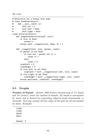
Longest Absolute Image File Path (Source. Leetcode 388) Sup-
pose we abstract our file system by a string in the following manner.
The string
dirntsubdir1nttfile1.extnttsubsubdir1ntsubdir2nttsubsubdir2ntttfile2.ext
represents:
dir
subdir1
file1.ext
subsubdir1
subdir2
subsubdir2
file2.png
74](https://image.slidesharecdn.com/codinginterviewpreparation-210311093651/85/Coding-interview-preparation-74-320.jpg)
![def solution(S):
S += ’n’
# Key: level
# Value: a tuple (most recent absolute path size at this
level, maximum absolute path size at this level)
dict = {}
dict[-1] = (0,0)
curLevelCount = 0
curFname =
for ch in S:
if ch != ’n’ and ch != ’ ’:
# Append new character if it is not a special character
curFname += ch
elif ch == ’n’:
curFnamePathSize = dict[curLevelCount-1][0] +
len(curFname)
if curLevelCount != 0:
# For the slash
curFnamePathSize += 1
pathSizeWeCare = curFnamePathSize - len(curFname)
if not (curFname.endswith(.jpeg) or
curFname.endswith(.png) or
curFname.endswith(.gif)):
pathSizeWeCare = 0
if curLevelCount in dict:
prevMax = dict[curLevelCount][1]
dict[curLevelCount] = (curFnamePathSize,
max(prevMax, pathSizeWeCare))
else:
dict[curLevelCount] = (curFnamePathSize,
pathSizeWeCare)
curFname =
curLevelCount = 0
else:
curLevelCount +=1
maxPathSize = 0
for level in dict:
if level = 0:
maxPathSize = max(maxPathSize, dict[level][1])
return maxPathSize
76](https://image.slidesharecdn.com/codinginterviewpreparation-210311093651/85/Coding-interview-preparation-76-320.jpg)
![Repeated Substring Pattern (Source. Leetcode 459) Given a non-
empty string check if it can be constructed by taking a substring of it and
appending multiple copies of the substring together. You may assume
the given string consists of lowercase English letters only and its length
will not exceed 10000. Difficulty: Easy. Examples:
Input: abab
Output: True
--
Input: abcabcabc
Output: False
Idea 1: There is a Greedy way to solve this by using the π table in the
KMP algorithm (refer to 2.8.2 for more description.) Once we have the
π table of the given string P, then P is a repetition of its substring if:
• π[|P|−1] ≥ (|P|−1)/2. Basically the longest prefix equal to suffix
must end beyond half of the string.
• The length of the given string, |P|, must be divisible by the pattern,
given by P0 · · · Pπ[|P| − 1]
class Solution(object):
def kmpTable(self, p):
... Check this code in appendix (5.2).
def repeatedSubstringPattern(self, s):
table = self.kmpTable(s)
if table[len(s)-1] (len(s)-1)/2:
return False
pattern = s[table[len(s)-1]+1:]
if len(s) % len(pattern) != 0:
return False
return True
Idea 2: There is a trick. Make a new string Q equal to the concatenation
of two given string P, so Q = P +P. Then, check if P is a substring of the
substring of Q, removing the front and last character, i.e. Q1 · · · Q|Q|−1.
Code:
def repeatedSubstringPattern(s):
q = s + s
return q[1:len(q)-1].find(s) != -1
77](https://image.slidesharecdn.com/codinginterviewpreparation-210311093651/85/Coding-interview-preparation-77-320.jpg)
![Valid Parenthesis Given a string containing just the characters ’(’,
’)’, ’’, ’’, ’[’ and ’]’, determine if the input string is valid.
The brackets must close in the correct order, ”()” and ”()[]” are all
valid but ”(]” and ”([)]” are not.
My code, using stack.
class Solution(object):
def isValid(self, s):
:type s: str
:rtype: bool
if len(s) % 2 != 0:
return False
pstart = {’(’: ’)’, ’{’: ’}’, ’[’: ’]’}
if s[0] not in pstart:
return False
recorder = []
for ch in s:
if ch in pstart:
recorder.append(ch)
else:
rch = recorder.pop()
if pstart[rch] != ch:
return False
return len(recorder) == 0
3.3 Permutation
There are several classic problems related to permutations. Some involve
strings, and some are just array of numbers.
Generate Parenthesis (Source. Leetcode 22) Given n pairs of paren-
theses, write a function to generate all combinations of well-formed
parentheses.
For example, given n = 3, a solution set is:
[
((())),
(()()),
78](https://image.slidesharecdn.com/codinginterviewpreparation-210311093651/85/Coding-interview-preparation-78-320.jpg)
![(())(),
()(()),
()()()
]
A bit strangely, I used iterative method. It was more intuitive for me
when I was doing this problem. My code:
class Solution(object):
def generateParenthesis(self, n):
S = {}
solution = []
S[’(’] = (1,0)
while True:
if len(S.keys()) == 0:
break
str, tup = S.popitem()
o, c = tup
if o == n:
if c == n:
solution.append(str)
continue
else:
S[str+’)’] = (o, c+1)
elif o == c:
S[str+’(’] = (o+1, c)
else:
S[str+’(’] = (o+1, c)
S[str+’)’] = (o, c+1)
return solution
Palindrome Permutations Given a string, determine if a permuta-
tion of the string could form a palindrome. For example, code -
False, aab - True, carerac - True..
This problem is relatively easy. Count the frequency of each character.
My code:
class Solution(object):
def canPermutePalindrome(self, s):
freq = {}
for c in s:
79](https://image.slidesharecdn.com/codinginterviewpreparation-210311093651/85/Coding-interview-preparation-79-320.jpg)
![if c in freq:
freq[c] += 1
else:
freq[c] = 1
if len(s) % 2 == 0:
for c in freq:
if freq[c] % 2 != 0:
return False
return True
else:
count = 0
for c in freq:
if freq[c] % 2 != 0:
count += 1
if count 1:
return False
return True
Next Permutation (Source. Leetcode 31) Implement next permuta-
tion, which rearranges numbers into the lexicographically next greater
permutation of numbers.
If such arrangement is not possible, it must rearrange it as the lowest
possible order (i.e., sorted in ascending order).
The replacement must be in-place, do not allocate extra memory.
Here are some examples. Inputs are in the left-hand column and its
corresponding outputs are in the right-hand column.
1,2,3 - 1,3,2
3,2,1 - 1,2,3
1,1,5 - 1,5,1
My code:
class Solution(object):
def _swap(self, p, a, b):
t = p[a]
p[a] = p[b]
p[b] = t
def nextPermutation(self, p):
if len(p) 2:
return
80](https://image.slidesharecdn.com/codinginterviewpreparation-210311093651/85/Coding-interview-preparation-80-320.jpg)
![if len(p) == 2:
self._swap(p, 0, 1)
return
i = len(p)-1
while i 0 and p[i-1] = p[i]:
i -= 1
# Want to increase the number at p[i-1]. That number
# should be the smallest one (but = p[i] in the range
# i to len(p)-1
if i 0:
smallest = p[i]
smallestIndex = i
for j in range(i, len(p)):
if p[j] p[i-1] and p[j] = smallest:
smallest = p[j]
smallestIndex = j
self._swap(p, i-1, smallestIndex)
# Reverse [i to len(p)-1)].
for j in range(i, i+(len(p)-i)/2):
self._swap(p, j, len(p)-1-(j-i))
3.4 Trees
Binary Tree Longest Consecutive Sequence (Source. Leetcode
298) Given a binary tree, find the length of the longest consecutive se-
quence path.
The path refers to any sequence of nodes from some starting node
to any node in the tree along the parent-child connections. The longest
consecutive path need to be from parent to child (cannot be the reverse).
Example:
1
3
/
2 4
5
Longest consecutive sequence path is 3-4-5, so return 3
81](https://image.slidesharecdn.com/codinginterviewpreparation-210311093651/85/Coding-interview-preparation-81-320.jpg)
![My code:
class Solution(object):
def __getRange(self, a, b):
if b - a 1:
if b - a == 2:
return str(a+1)
else:
return str(a+1) + - + str(b-1)
else:
return None
def findMissingRanges(self, nums, lower, upper):
result = []
upper += 1
lower -= 1
lastOne = lower
if len(nums) 0:
lastOne = nums[len(nums)-1]
for i, n in enumerate(nums):
rg = None
if i == 0:
# First number
rg = self.__getRange(lower, nums[0])
else:
rg = self.__getRange(nums[i-1], nums[i])
if rg is not None:
result.append(rg)
# Last number
rg = self.__getRange(lastOne, upper)
if rg is not None:
result.append(rg)
return result
3.6 Divide and Conquer
Median of Two Sorted Arrays (Source. Leetcode 4) There are two
sorted arrays nums1 and nums2 of size m and n respectively.
Find the median of the two sorted arrays. The overall run time com-
plexity should be O(log(m + n)).
83](https://image.slidesharecdn.com/codinginterviewpreparation-210311093651/85/Coding-interview-preparation-83-320.jpg)
![This is a hard problem. I have two blog posts about two different ap-
proaches to find k-th smallest elements in two sorted arrays:
• Recursive O(log(mn)):
http://zkytony.blogspot.com/2016/09/find-kth-smallest-element-in-two-sorted.html
• Recursive O(logk)):
http://zkytony.blogspot.com/2016/09/find-kth-smallest-element-in-two-sorted_19.
html
My code:
class Solution(object):
def findMedianSortedArrays(self, nums1, nums2):
n = len(nums1)
m = len(nums2)
if (n+m) % 2 == 0:
m0 = self.kth(nums1, nums2, (n+m)/2-1)
m1 = self.kth(nums1, nums2, (n+m)/2)
return (m0 + m1) / 2.0
else:
return self.kth(nums1, nums2, (n+m)/2)
def kth(self, A, B, k):
if len(A) len(B):
A, B = (B, A)
if not A:
return B[k]
if k == len(A) + len(B) - 1:
return max(A[-1], B[-1])
i = min(len(A)-1, k/2)
j = min(len(B)-1, k-i)
if A[i] B[j]:
return self.kth(A[:i], B[j:], i)
else:
return self.kth(A[i:], B[:j], j)
3.7 Dynamic Programming
Paint Fence There is a fence with n posts, each post can be painted
with one of the k colors.
84](https://image.slidesharecdn.com/codinginterviewpreparation-210311093651/85/Coding-interview-preparation-84-320.jpg)
![You have to paint all the posts such that no more than two adjacent
fence posts have the same color.
Return the total number of ways you can paint the fence. Note that
n and k are non-negative integers.
My code29
:
class Solution(object):
def numWays(self, n, k):
if n == 0:
return 0
if n == 1:
return k
# Now n = 2.
# Initialize same and diff as if n == 2
same = k
diff = k*(k-1)
for i in range(3,n+1):
r_prev = same + diff # r(i-1)
same = diff # same(i)=diff(i-1)
diff = r_prev*(k-1)
return same + diff
3.8 Miscellaneous
Range Sum Query 2D - Mutable (Source. Leetcode 308) Given
a 2D matrix matrix, find the sum of the elements inside the rectangle
defined by its upper left corner (row1, col1) and lower right corner (row2,
col2). Difficulty: Hard. Example:
Given matrix = [
[3, 0, 1, 4, 2],
[5, 6, 3, 2, 1],
[1, 2, 0, 1, 5],
[4, 1, 0, 1, 7],
[1, 0, 3, 0, 5]
]
sumRegion(2, 1, 4, 3) - 8
29I have a blog post about this problem: http://zkytony.blogspot.com/2016/09/
paint-fence.html
85](https://image.slidesharecdn.com/codinginterviewpreparation-210311093651/85/Coding-interview-preparation-85-320.jpg)
![//The above rectangle (with the red border) is defined by (row1,
col1) = (2, 1) and (row2, col2) = (4, 3), which contains sum
= 8.
update(3, 2, 2)
sumRegion(2, 1, 4, 3) - 10
Idea: Use binary indexed tree. This kind of tree is built to solve problems
like this. See 2.1.15 for more detailed explanation of how it works. Code
is below. The formula to compute parent index of an index i, parent(i)
= i+i(-i), not only works for 1D array, but also for the row and
column index for 2D array.
class BinaryIndexTree():
def __init__(self, matrix):
if not matrix:
return
self.num_rows = len(matrix)+1
self.num_cols = len(matrix[0])+1 if len(matrix) 0 else 0
self.matrix = [[0 for x in range(self.num_cols-1)] for y
in range(self.num_rows-1)]
self.tree = [[0 for x in range(self.num_cols)] for y in
range(self.num_rows)]
for r in range(self.num_rows-1):
for c in range(self.num_cols-1):
self.update(r, c, matrix[r][c])
def update(self, row, col, val):
i = row + 1
while i self.num_rows:
j = col + 1
while j self.num_cols:
self.tree[i][j] += val - self.matrix[row][col]
j += ((~j+1) j)
i += ((~i+1) i)
self.matrix[row][col] = val
def sum(self, row, col):
result = 0
i = row + 1
while i 0:
j = col + 1
while j 0:
result += self.tree[i][j]
86](https://image.slidesharecdn.com/codinginterviewpreparation-210311093651/85/Coding-interview-preparation-86-320.jpg)
![Input:
rows = 3, cols = 6, sentence = [a, bcd, e]
Output:
2
Explanation:
a-bcd-
e-a---
bcd-e-
The character ’-’ signifies an empty space on the screen.
Trapping Rain Water (Source. Leetcode 42) Given n non-negative
integers representing an elevation map where the width of each bar is 1,
compute how much water it is able to trap after raining.
For example, Given [0,1,0,2,1,0,1,3,2,1,2,1], return 6. Visu-
alize it yourself.
Trapping Rain Water 2D (Source. Leetcode 407) Given an m x n
matrix of positive integers representing the height of each unit cell in a
2D elevation map, compute the volume of water it is able to trap after
raining. Example:
Given the following 3x6 height map:
[
[1,4,3,1,3,2],
[3,2,1,3,2,4],
[2,3,3,2,3,1]
]
Return 4.
Visualize this matrix by drawing a 3D image based off of a 2D grid base.
Each grid extends upwards by height specified in the corresponding cell
in the matrix.
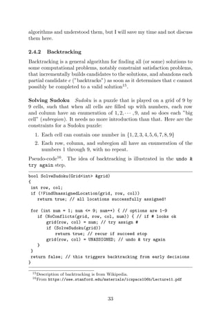
Implement pow(x, n) Implement the power frunction.
88](https://image.slidesharecdn.com/codinginterviewpreparation-210311093651/85/Coding-interview-preparation-88-320.jpg)
![Find Minimum in sorted rotated array Suppose an array sorted
in ascending order is rotated at some pivot unknown to you beforehand.
(i.e., 0 1 2 4 5 6 7 might become 4 5 6 7 0 1 2). Find the mini-
mum element. You may assume no duplicate exists in the array.
Follow-up: What if duplicates are allowed?
The Skyline Problem (Source. Leetcode 218) A city’s skyline is
the outer contour of the silhouette formed by all the buildings in that
city when viewed from a distance. Now suppose you are given the
locations and height of all the buildings as shown on a cityscape
photo (Figure A), write a program to output the skyline formed by
these buildings collectively (Figure B).
The geometric information of each building (input) is represented by
a triplet of integers [Li, Ri, Hi], where Li and Ri are the x coordinates
of the left and right edge of the ith building, respectively, and Hi is its
height.
For instance, the dimensions of all buildings in Figure A are recorded
as: [ [2 9 10], [3 7 15], [5 12 12], [15 20 10], [19 24 8] ]
.
The output is a list of ”key points” (red dots in Figure B) in the for-
mat of [ [x1,y1], [x2, y2], [x3, y3], ... ] that uniquely de-
fines a skyline. A key point is the left endpoint of a horizontal line
89](https://image.slidesharecdn.com/codinginterviewpreparation-210311093651/85/Coding-interview-preparation-89-320.jpg)
![segment. Note that the last key point, where the rightmost building
ends, is merely used to mark the termination of the skyline, and always
has zero height. Also, the ground in between any two adjacent buildings
should be considered part of the skyline contour.
For instance, the skyline in Figure B should be represented as:[ [2
10], [3 15], [7 12], [12 0], [15 10], [20 8], [24, 0] ].
Notes:
1. The input list is already sorted in ascending order by the left x
position Li.
2. The output list must be sorted by the x position.
3. There must be no consecutive horizontal lines of equal height in the
output skyline. For instance, [...[2 3], [4 5], [7 5], [11
5], [12 7]...] is not acceptable; the three lines of height 5
should be merged into one in the final output as such: [...[2
3], [4 5], [12 7], ...]
Minimum Path Sum (Source. Leetcode 64) Given a m×n grid filled
with non-negative numbers, find a path from top left to bottom right
which minimizes the sum of all numbers along its path. Note: You can
only move either down or right at any point in time.
Minimum Height Trees (Source. Leetcode 310) For a undirected
graph with tree characteristics, we can choose any node as the root.
The result graph is then a rooted tree. Among all possible rooted trees,
those with minimum height are called minimum height trees (MHTs).
Given such a graph, write a function to find all the MHTs and return a
list of their root labels.
Format: The graph contains n nodes which are labeled from 0 to n -
1. You will be given the number n and a list of undirected edges (each
edge is a pair of labels).
You can assume that no duplicate edges will appear in edges. Since
all edges are undirected, [0, 1] is the same as [1, 0] and thus will not
appear together in edges.
Closest Binary Search Tree Value (Source. Leetcode 270) Given
a non-empty binary search tree and a target value, find the value in the
BST that is closest to the target.
90](https://image.slidesharecdn.com/codinginterviewpreparation-210311093651/85/Coding-interview-preparation-90-320.jpg)
![Wiggle Sort (Source. Leetcode 324) Given an unsorted array nums,
reorder it in-place such that nums[0] = nums[1] = nums[2] = nums[3]....
For example, given nums = [3, 5, 2, 1, 6, 4], one possible an-
swer is [1, 6, 2, 5, 3, 4].
Wiggle Sort II (Source. Leetcode 324) Given an unsorted array
nums, reorder it such that nums[0] nums[1] nums[2] nums[3]....
For example, given nums = [1, 3, 2, 2, 3, 1], one possible an-
swer is [2, 3, 1, 3, 1, 2].
Number of Islands II A 2d grid map of m rows and n columns
is initially filled with water. We may perform an addLand operation
which turns the water at position (row, col) into a land. Given a list
of positions to operate, count the number of islands after each addLand
operation. An island is surrounded by water and is formed by connecting
adjacent lands horizontally or vertically. You may assume all four edges
of the grid are all surrounded by water.
See 3.5 for the first version of Number of Islands problem.
Word Squares Given a set of words (without duplicates), find all
word squares you can build from them.
A sequence of words forms a valid word square if the kth row and col-
umn read the exact same string, where 0 ≤ k ≤ max(numRows, numColumns).
For example, the word sequence [ball,area,lead,lady]
forms a word square because each word reads the same both horizontally
and vertically.
b a l l
a r e a
l e a d
l a d y
All words will have the exact same length. Word length is at least 1 and
at most 5. Each word contains only lowercase English alphabet a-z.
Go to Leetcode for more questions.
91](https://image.slidesharecdn.com/codinginterviewpreparation-210311093651/85/Coding-interview-preparation-91-320.jpg)
![4 Behavioral
4.1 Standard
4.1.1 introduce yourself
This question is an ice breaker. For this kind of question, the most
important points to hit are (1) What is your interest in software en-
gineering, (2 Very briefly say your background; don’t be too detailed
because that will take up too much time in the interview. Be yourself.
Be natural. I will probably say something as follows.
I major in Computer Science. I am expected to graduate in June,
2017. I am interested in backend or fullstack software develop-
ment. I also hope to do work that involves some flavor of research,
because I love doing research. I am also interested in using ma-
chine learning to solve some of problems I will work on. I am
currently working at the Robotics State-Estimation Lab at UW.
I can talk more about that project later. [(but) The big parts
that I’ve contributed is that I’ve improved the navigation system
for our robot, and also made a pipeline for data collection of the
deep learning model.]This part can be omitted Besides robotics, I am
also leading a group of 4 to work on the Koolio project, a web-
site for people to share flippable content. In the last summer, I
worked at CME Group for basically full stack development of a
web application for helping my PM creating JIRA subtickets for
the upcoming sprint (2 weeks). I think I am well prepared to be
able to work at Google.
4.1.2 talk about your last internship
Here is what I may say:
I interned at CME Group. The goal of the project that I worked
on, solo, was to develop a web app to help replace my project
manager’s heavy Excel sheet work flow. Part of the Excel work
flow involved creating ”work types” which are basically cartesian
product of several sets of short names such as ”Front”, ”Back”
as a set, ”Dev”, ”Test” as a set, etc. So part of the functionality
I implemented was to let the user configure the work types, save
them into a database, and then use those to assign people tasks
in another interface I made. This project used JavaScript, Java
and Groovy on Grails, which is a Spring MVC under the hood. I
also learned some knowledge in finance, and saw the closing of the
92](https://image.slidesharecdn.com/codinginterviewpreparation-210311093651/85/Coding-interview-preparation-92-320.jpg)
![Chicago Mercantile Exchange physical place, and the transition
to high-frequency online trading.
4.1.3 talk about your current research
Here is what I may say. Depending on the level of detail expected, I will
vary my answer.
I started working at the lab in April, 2016, supervised by Post-
doc Andrzej Pronobis and Professor Rajesh Rao. The goal of
our project is to develop a novel probabilistic framework that en-
ables robots to learn a unified deep generative model that captures
multiple layers of abstraction, which is essentially one model that
does the job of several independent ones such as place recogni-
tion, object detection, or action modeling. The motivation is that
although those single models work well, they each require huge
computation power, and they exchange information in a limited
way.
The two main components that I have been in charge of are (1)
mobile robot navigation, (2) design and development of a pipeline
for representation learning of the deep learning model, which can
collect virtual scans of the environment from the robot’s sensor
readings. I worked on both components independently. I was
acknowledged for my help in collecting the data in the ICRA 2017
paper. I also have video demo of the navigation on the robot, and
also contributed a navigation tuning guide to ROS community.
I’m expected to work on simulated world generation soon.
4.1.4 talk about your projects
I will talk about Koolio, for sure.
The biggest side project I have been working on is the Koolio.io.
Koolio.io is a website where users can share and view two-sided
flippable cards. You may be tempted to know what’s on the other
side of a card, or you may just flip around as you enjoy. So the
central core of this site is entertainment, in a unique form. [A piece
of information has value as long as it is entertaining to people.]Can
be omitted
When creating a card, user can decide what type of content to
put on each side of it (we support text, image, and video for now).
A deck groups multiple cards together, indicating their topic.
93](https://image.slidesharecdn.com/codinginterviewpreparation-210311093651/85/Coding-interview-preparation-93-320.jpg)

![def kmpTable(p):
i, j = 1, 0
table = {-1: -1, 0: -1}
while i len(p):
if p[i] == p[j]:
table[i] = j
j += 1
i += 1
else:
if j 0:
j = max(0, table[j-1] + 1)
else:
table[i] = -1
i += 1
return table
def kmp(W, P):
table = kmpTable(P)
k = 0
while k len(W):
d = 0
j = k
# Check if the remaining string is long enough
if len(W) - k len(P):
return -1
for i in range(0, len(P)):
if P[i] == W[j]:
d += 1
j += 1
else:
break # mismatch
# KMP rules
if d == len(P):
return k
elif d 0 and table[d-1] == -1:
k = k + d
elif d 0 and table[d-1] != -1:
k = k + d - table[d-1] - 1
else: # d == 0
k = k + 1
return -1
99](https://image.slidesharecdn.com/codinginterviewpreparation-210311093651/85/Coding-interview-preparation-99-320.jpg)
![5.3 Python Implementation of Union-Find
Based on details described in 2.1.16, I implemented the Union-Find data
structure in python as follows.
class UnionFind:
Caveat: This implementation does not support adding
additional elements other than ones given initially.
def __init__(self, elems):
Constructs a union find data structure. Assumes that all
elements in elems are hashable.
self.elems = list(elems)
self.idxmap = {}
self.impl = []
for i in range(len(elems)):
self.idxmap[self.elems[i]] = i
self.impl.append(-1)
def find(self, x):
return the canonical name of the set that element x
belongs to
if self.__implVal(x) 0:
return x
return self.find(self.elems[self.__implVal(x)])
def union(self, x, y):
union the two sets that each of x and y is in.
# We want |s(c1)| = |s(c2)|. Here, s(N) means the set
represented by the canonical element N.
c1, c2 = self.find(x), self.find(y)
if c1 == c2:
return c1 # already unioned
s1, s2 = abs(self.__implVal(c1)), abs(self.__implVal(c2))
if s1 s2:
c1, c2 = c2, c1
self.impl[self.idxmap[c1]] = self.idxmap[c2] # Connect.
self.impl[self.idxmap[c2]] = -(s1 + s2) # Update the size.
return c2 # Return the canonical element of the new set.
def __implVal(self, x):
return self.impl[self.idxmap[x]]
100](https://image.slidesharecdn.com/codinginterviewpreparation-210311093651/85/Coding-interview-preparation-100-320.jpg)