Hidrogeologia

1. COMPSEC, a new tool to derive natural background levels by the
component separation approach: application in two different
hydrogeological contexts in northern Italy
Marco Rotiroti a,
⁎, Biagio Di Mauro b
, Letizia Fumagalli a
, Tullia Bonomi a
a
Department of Earth and Environmental Sciences, University of Milano-Bicocca, Piazza della Scienza 1, 20126 Milano, Italy
b
Remote Sensing of Environmental Dynamics Lab., Department of Earth and Environmental Sciences, University of Milano-Bicocca, Piazza della Scienza 1, 20126 Milano, Italy
a b s t r a c t
a r t i c l e i n f o
Article history:
Received 20 October 2014
Revised 18 May 2015
Accepted 24 June 2015
Available online 4 July 2015
Keywords:
Natural background levels
Component separation
Pre-selection
Groundwater quality
Cremona
Aosta
The assessment of natural background levels (NBLs) is crucial in the management of groundwater resources and
the definition of the status of groundwater bodies according to the Water Framework Directive 2000/60/EC. This
work presents a new MATLAB code to assess NBLs by the component separation method, which concerns the
identification and separation of a natural and an anthropogenic component within geochemical data. To increase
the validity of the estimated NBL, the code calculates a set of possible solutions that should then be evaluated by
the user. The following evaluation criteria are proposed: (i) stability of solution, (ii) hydrogeochemical reliability,
(iii) agreement with the conceptual model and (iv) goodness of fit.
The code is tested on groundwater Mn, Fe, As, Ni, Cr(VI) and NH4 concentrations observed in two study areas
with different hydrogeological and geochemical features in northern Italy: the multi-layer aquifer of Cremona
(lower Po Plain) and the alluvial aquifer of the Aosta Plain (western Alpine sector). The pre-selection method
is also applied to estimate NBLs and threshold values are assessed.
The NBLs calculated through the component separation method (4292, 27 and 1220 μg/L for Fe, As and NH4 in
Cremona and 56, 261, 9 and 2.3 μg/L for Mn, Fe, Ni and Cr(VI) in Aosta, respectively) approach those estimated
by the pre-selection (2798, 25 and 1820 μg/L for Fe, As and NH4 in Cremona and 52, 264, 10 and 1.8 μg/L for
Mn, Fe, Ni and Cr(VI) in Aosta, respectively). This outcome increases the validity of the estimated NBLs. The
code showed versatile applicability in different contexts and conditions (e.g., different numbers of samples and
monitoring points, different sampling networks). This work highlights the strength of the component separation
method although some criticisms are pointed out, mainly related to the superimposition of a log-normal function
for modeling the natural component.
© 2015 Elsevier B.V. All rights reserved.
1. Introduction
The EU Water Framework Directive (WFD 2000/60/EC) requires
Member States to assess the status of groundwater bodies to achieve
good groundwater status within 2015. In those areas where naturally
high concentrations of undesirable elements exist, the chemical status
is evaluated through a comparison with threshold values (TVs) that
are estimated on the basis of natural background levels (NBLs). Accord-
ing to the Water Framework Directive, the TV is defined as a quality
standard for pollutants in groundwater, i.e., a concentration of pollutant
which should not be exceeded in order to protect human health and the
environment. Although TVs and NBLs are crucial in environmental man-
agement, they are theoretical values whose geochemical meaning
cannot reliably be derived from experimental data. To fill this gap,
different methods and approaches have been developed in the last
decades, with continuous updates. A general subdivision of proposed
methodologies for deriving NBL discriminates between geochemical
and statistical methods (Gałuszka, 2007; Matschullat et al., 2000).
The geochemical methods involve the derivation of NBLs as a fixed
value (typically mean, median or 90th percentile) calculated from
groundwater samples that can be considered free from anthropogenic
impacts. Some examples of undisturbed datasets are: (i) samples from
deeper aquifers (Muller et al., 2006); (ii) samples of non-recent ground-
water (i.e., groundwater with no tritium) (Griffioen et al., 2008); (iii)
historical datasets referring to periods in which anthropogenic activities
generated no significant impacts (i.e., before 1945) (Griffioen et al.,
2008). The calculation of NBLs via hydrogeochemical modeling of solu-
tion processes in aquifers (Muller et al., 2006) can also be considered as
part of the geochemical methods.
The statistical methods include various techniques aimed at identi-
fying and extracting a natural background population (NBP) from the
experimental data. The NBP can be representative of the undisturbed nat-
ural condition of a groundwater body. The NBL is then derived using
Journal of Geochemical Exploration 158 (2015) 44–54
⁎ Corresponding author.
E-mail address: m.rotiroti@campus.unimib.it (M. Rotiroti).
http://dx.doi.org/10.1016/j.gexplo.2015.06.017
0375-6742/© 2015 Elsevier B.V. All rights reserved.
Contents lists available at ScienceDirect
Journal of Geochemical Exploration
journal homepage: www.elsevier.com/locate/jgeoexp

2. statistical parameters characterizing the NBP. Although a unique value is
frequently needed for environmental management (e.g., remediation
goals, TV for defining chemical status), the NBL is typically expressed
through a range of concentration values (e.g., mean ± 2 standard devi-
ation and median ± 2 median absolute deviation) (Matschullat et al.,
2000; Reimann et al., 2005). A key aspect is what type of distribution
(i.e., normal or log-normal) should be selected for the NBP, regardless
of the distribution of the original experimental data, which frequently
show no normal or log-normal characteristics (Reimann and Filzmoser,
2000). Some methods consider a normal distribution for the NBP, as-
suming that each process acting in the system produces on the whole
data fluctuating around a mean value and with normally distributed er-
rors (Matschullat et al., 2000; Nakić et al., 2010). Statistical methods
that aim to identify normally distributed NBP are: (i) the iterative 2δ-
technique (Matschullat et al., 2000), where an approximated normally
distributed NBP is generated around the modal value of the original
dataset; some applications are in Gałuszka (2007), Nakić et al. (2007,
2010) and Urresti-Estala et al. (2013); (ii) the calculated distribution
function (Matschullat et al., 2000), where the NBP is generated from
the original data taking the range between the minimum and the medi-
an and their “mirrored” values against the original median; some exam-
ples are reported by Nakić et al. (2007, 2010) and Urresti-Estala et al.
(2013); (iii) the modal analysis (Carral et al., 1995), that decomposes
the polymodal distribution of the original data into several normal dis-
tributions by a maximum likelihood mixture estimation (MLME) and
then considers the normal distribution of the lowest mean value as
NBP; some applications are in Carballeira et al. (2002), Rodríguez et al.
(2006) and Villares et al. (2002). Other statistical methods consider a
log-normal distribution for the NBP, following the assumption that nat-
ural geochemical data are typically log-normally distributed (Ahrens,
1953; Gaddum, 1945; Limpert et al., 2001). From this class of methods,
particular relevance is provided by the component separation (CS) ap-
proach (Wendland et al., 2005) which involves the subdivision of the
original dataset into a normally and a log-normally distributed popula-
tion, considering the latter as NBP; some examples are reported by
Molinari et al. (2012, 2014). The latter class of methods is independent
of both a normal and a log-normal distribution for the NBP. These
methods are: (i) the probability plot (Sinclair, 1974), where the NBP
is graphically extracted from the original data onto a cumulative proba-
bility plot; some examples were reported by Panno et al. (2006),
Preziosi et al. (2014) and Tobías et al. (1997); (ii) the fractal method
(Cheng et al., 1994), that takes into account the spatial variability of
geochemical data using the power law concentration-area analysis
(Albanese et al., 2007; Li et al., 2003); (iii) the pre-selection (PS) ap-
proach (Muller et al., 2006), where the NBP is extracted from the origi-
nal data by excluding the samples with most likely anthropogenic
influences identified using indicator chemical species (Hinsby et al.,
2008; Wendland et al., 2008a).
Among these different methodologies, the EU BRIDGE research pro-
ject (Background cRiteria for the IDentification of Groundwater thrEsh-
olds) (Muller et al., 2006) provides guidelines aiming at harmonizing
the methods for estimating the NBL at the European level. The BRIDGE
project mainly focuses on two different approaches: PS and CS. While
several applications of PS are reported in literature (Coetsiers et al.,
2009; Ducci and Sellerino, 2012; Gemitzi, 2012; Hinsby et al., 2008;
Marandi and Karro, 2008; Molinari et al., 2012; Preziosi et al., 2010,
2014; Rotiroti and Fumagalli, 2013; Wendland et al., 2008a), a few stud-
ies concern the use of CS (Molinari et al., 2012, 2014; Voigt et al., 2005;
Wendland et al., 2005). The limited use of CS among researchers and
public administrations may be due to the absence of a standard statisti-
cal package for its application.
This paper presents a MATLAB® code, called COMPonent SEparation
Code (COMPSEC), which aims to estimate the NBL using the CS ap-
proach through a maximum likelihood estimation (MLE). The perfor-
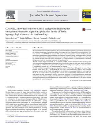
mance of COMPSEC is tested here in two different case studies in
northern Italy (Fig. 1): (i) the multi-layer aquifer of Cremona (lower
Po Plain) and (ii) the alluvial aquifer of the Aosta Plain (N/W Alpine
sector). These two study areas also differ in the characteristics of the
sampling network: unevenly distributed (highly clustered) samples in
Cremona and homogeneously distributed samples in Aosta (Fig. 1). To
compare the results from both approaches proposed by BRIDGE, the
NBLs are derived by both PS and CS approaches, then the NBLs are com-
pared to the regulatory references (REFs) for estimating the TV.
2. Conceptual model of study areas
The elaboration of proper hydrogeological and hydrogeochemi-
cal conceptual models of the groundwater bodies investigated
(i.e., hydrogeological features of the aquifer, presence of anthropogenic
sources and hydrogeochemical processes governing the mobility of the
chemical species) plays an important role in the estimation of the NBLs
(Hinsby et al., 2008; Molinari et al., 2014; Muller, 2008; Muller et al.,
2006; Preziosi et al., 2014; Wendland et al., 2008b). The conceptual
models for the two areas investigated are illustrated in the following
sections.
2.1. Cremona area
The Cremona area is located on the lower Po Plain (N Italy) and is
bounded to the south by the Po River (Fig. 1b). It covers a 50 km2
area
around the town of Cremona. The subsurface is composed of alluvial
sediments deposited during the Holocene and Pleistocene. The transi-
tion between outcropping Holocene and Pleistocene deposits is marked
by a fluvial terrace (Castiglioni et al., 1997) which crosses the area from
W to E (Fig. 1b). The zone south of the terrace scarp (Holocene unit) cor-
responds to the fluvial valley of the Po River, whereas the zone north of
the terrace (Pleistocene unit) is associable with the Main Level of Po
Plain (Petrucci and Tagliavini, 1969). A detailed structure of the aquifer
system of the Cremona area is reported in previous studies by Rotiroti
et al. (2012a, 2014), where the interpretation of lithostratigraphic data
together with measured hydraulic heads leads to the identification of
five aquifer units: (i) unconfined from 0 to 25 m below surface,
(ii) semi-confined from 30 to 50 m, (iii) confined 1 from 65 to 85 m,
(iv) confined 2 from 100 to 150 m and (v) confined 3 from 160 to
250 m. The subject of this work is only the shallowest unconfined aqui-
fer, which is more vulnerable to anthropogenic pollution. Here, the
discrimination between natural and anthropogenic components for a
given contamination is crucial in guaranteeing proper protection and
management of water resources.
The unconfined aquifer is recharged by precipitation, irrigation and
drainage of surface water (irrigation canals) and discharges into the
Po River and by groundwater extraction (Vassena et al., 2012). The
main groundwater direction is N/S (Beretta et al., 1992; Vassena et al.,
2012), controlled by topography and the Po River, which mainly gains
groundwater (Rotiroti et al., 2014). Shallow groundwater is generally
of the Ca-HCO3 type with an average pH and alkalinity of ~7.3 and
~460 mg/L as HCO3; mean concentrations of NO3, Cl, SO4, Ca, Mg, K
and Na are 21, 27, 71, 165, 28, 1.7 and 18, respectively (Rotiroti et al.,
2014). The unconfined aquifer is characterized by hydrochemical zon-
ing (Fig. 1b): the Main Level of Po Plain has oxidized hydro-facies,
whereas the Po Valley has reduced hydro-facies with high concentra-
tions of As, Fe, Mn and NH4 (Rotiroti and Fumagalli, 2013), which
exceed the Italian regulatory limits of 10, 200, 50 and 500 μg/L, respec-
tively (Legislative Decree 152/06; Legislative Decree 30/09). These
hydrochemical features are probably related to the geological settings.
The Main Level of Po Plain is mainly composed of shallow sandy de-
posits that allow the infiltration of oxidized water (rainwater), whereas
the Po Valley is characterized by the presence of shallow silty-clayey de-
posits that limit infiltration and aquifer recharge, and of abundant peat
deposits, generated by the meandering and flooding activities of the Po
River. Peat deposits are known to act as redox drivers of As release to
groundwater, as well as for Fe and Mn (McArthur et al., 2001, 2004;
45
M. Rotiroti et al. / Journal of Geochemical Exploration 158 (2015) 44–54

3. Postma et al., 2007; Rowland et al., 2006), since the oxidation of peat or-
ganic carbon is coupled with the reductive dissolution of Mn and Fe
oxide-hydroxides, where As is commonly sorbed (Ravenscroft et al.,
2009). These processes are assumed to occur in the Po Valley (Rotiroti
et al., 2012b, 2014). In particular, following the ecological succession
of electron acceptors (O2, NO3, Mn(IV)-oxide, Fe(III)-oxide, SO4 and
CO2), it is expected to have a first mobilization of Mn, followed by Fe
and finally by As, which is strongly released to groundwater only after
sufficient Fe has been reduced (McArthur et al., 2004; Ravenscroft
et al., 2009).
The Cremona area is impacted by urban and industrial activities
(steelworks, oil refinery, food industry), and thus, anthropogenic con-
taminations may occur. In particular, since no direct anthropogenic
sources of As, Fe and Mn exist in the area, attention focuses on pollution
by organic matter, which can indirectly influence the concentrations of
dissolved As, Fe and Mn (Baedecker et al., 1993; Berbenni et al., 2000;
Burgess and Pinto, 2005; Tuccillo et al., 1999). Three sites with possible
anthropogenic influences on As, Fe, Mn and NH4 concentrations have
been identified in the Cremona area, particularly in the Po Valley:
(i) an oil refinery with relevant hydrocarbon pollution, (ii) a municipal
solid waste landfill with most likely leachate spills and (iii) a group of
petrol stations with small hydrocarbon spills. Concerning NH4, only
the landfill can be considered as a site with possible influences since
NH4 and organic-N are generally absent in hydrocarbons owing to
their release in hydrocarbon formation and maturation (Williams
et al., 1992). Since the three sites are all located in the Po Valley, they
are part of the reduced zone of the unconfined aquifer. Therefore, in
this zone, an anthropogenic component in addition to the natural com-
ponent is expected for As, Fe, Mn and NH4 concentrations.
2.2. Aosta area
The Aosta area (~40 km2
) is located on the Aosta Plain, an Alpine val-
ley extending east-westward along 32 km and crossed by the Dora
Baltea River in the Aosta Valley Region in NW Italy (Fig. 1c). The basin
was filled by glacial, lacustrine, alluvial and fan deposits in the Pleisto-
cene and Holocene. A silty layer of lacustrine origin is located at ~80 m
of depth and is the aquiclude of the system (Bonomi et al., 2013; Novel
et al., 2002). A unique unconfined aquifer exists in the western part of
the area (west of the town of Aosta) whereas a subdivision into an uncon-
fined upper aquifer and a semiconfined deeper aquifer occurs in the east-
ern part due to a second silty lacustrine layer at ~20 m of depth (Bonomi
et al., 2013; De Maio et al., 2009; Novel et al., 2002).
The aquifer system is recharged by infiltration (rainwater and snow
melt) which is higher in the alluvial fans located at the edge of the plain,
surface water (springs and tributaries of the Dora Baltea River), lateral
inflow from fractured bedrock and discharges by downstream outflow
and well extraction (Bonomi et al., 2013; Novel et al., 2002). A key
role in the water balance of the aquifer system is played by the Dora
Baltea River which loses upstream of the town of Aosta and gains down-
stream (Bonomi et al., 2013). The main groundwater flow direction is
W/E and is influenced by the gaining behavior of the Dora Baltea River
downstream of Aosta. Groundwater is mainly of the Ca-HCO3 type
although a shift toward the SO4-HCO3 type is evidenced in the
Charvensod area, south of the town of Aosta, likely due to the interac-
tion with evaporites (gypsum and anhydrite) (Novel et al., 2002). The
concentration of major ions is in accordance with typical values found
in natural groundwater systems, indeed the average concentrations of
alkalinity (as HCO3), NO3, Cl, SO4, Ca, Mg, K, Na and pH are respectively
219, 7, 25, 89, 86, 16, 3.2, 12 mg/L and 7.4 (data from the available
dataset, see Section 3.1.2). Concerning the unconfined aquifer, both in
the western (unique body) and eastern (shallower aquifer) zones, an
oxidized hydro-facies is dominant, although sporadic high concentra-
tions of Fe and Mn (exceeding the limit of Legislative Decree 152/06)
are found. The occurrence of Fe and Mn in groundwater of the Aosta
Plain may be related to the mineralization of the organic matter
contained in the lacustrine deposits. The importance of redox processes,
driven by the lacustrine organic matter, on the hydrochemical features
of groundwater in the Aosta Plain is also highlighted by the isotope anal-
ysis by Novel et al. (2002). Another key aspect is the presence of concen-
trations of the trace elements Cr(VI) and Ni exceeding the regulatory
limits (Legislative Decree 30/09) of 5 and 20 μg/L, respectively. These
high concentrations are mainly located in the eastern part of the Aosta
Plain and are likely natural, related to the mineralogical composition
Fig. 1. (a) Digital elevation model of northern Italy and study areas. (b) Cremona area: sampling points and redox zoning. (c) Aosta area: sampling points.
46 M. Rotiroti et al. / Journal of Geochemical Exploration 158 (2015) 44–54

4. of the aquifer matrix in that area, which is characterized by ophiolites
and serpentinites (De Giusti et al., 2003).
Similar to the Cremona area, the Aosta area has urban and industrial
activities which can decrease overall groundwater quality, particularly
in the zone close to the town of Aosta, where an industrial area with
an elevated pollution risk is identified (De Maio et al., 2010). In particu-
lar, this industrial area and the downstream sector are characterized by
an anthropogenic plume of Cr(VI) (Capodaglio, 2005). An anthropogen-
ic influence may also derive from some old non-controlled landfills
located east of the town of Aosta (Brissogne landfills), particularly on
Fe and Mn concentrations.
3. Materials and methods
3.1. Available datasets
3.1.1. Cremona
The hydrochemical data were collected from the Province of Cremo-
na, specifically from the archives of the office charged with remediation
of polluted sites. The total dataset is composed of the sum of several
site-specific monitoring networks, each with a different number and
density of sampling points and measured chemical parameters. Typical-
ly, only a few species were measured in each sample, in relation to the
specific groundwater quality problem of each site. The dataset collected
for this work contains only measured concentrations of As, Fe, Mn and
NH4 for each sample, with no measures of major anions and cations.
Since the selected species were measured on filtered samples, their con-
centrations indicate the dissolved content. The whole dataset refers to
the 1997–2010 period. The temporal resolution of samples is also un-
even depending on the case of pollution of each site (from monthly
samples over a whole year to a single sample per well). The total num-
ber of samples and monitoring points in the unconfined aquifer is 773
and 176 for Mn, 773 and 175 for Fe, 663 and 158 for As and 277 and
76 for NH4, respectively. The number of samples and monitoring points
subdivided into oxidized and reduced zones, together with main statis-
tical parameters for measured concentrations, is shown in Table 1. The
average number of samples for each point for Mn, Fe, As and NH4 is
4.4, 4.4, 4.2 and 3.6, with maxima of 25, 25, 24 and 14, respectively.
3.1.2. Aosta
The acquired data are part of the hydrochemical databases of the Re-
gional Environmental Protection Agency of Aosta Valley (ARPA). In par-
ticular, the present work focuses on the samples from the groundwater
quality monitoring network, referring to the 1998–2012 period. The
temporal resolution is generally six months (one sample in summer
and one in winter). Unlike the Cremona area, the selected species (Fe,
Mn, Ni and Cr(VI)) were measured from unfiltered samples, thus their
concentrations indicate total content. In addition to the selected species,
the available dataset also includes the measures of major anions and
cations for each sample. The dataset refers to the unconfined aquifer
of the Aosta Plain. The total number of samples and monitoring points
is 1147 and 129 for Mn and Fe, 1136 and 128 for Ni and 1095 and 117
for Cr(VI), respectively. The main statistical parameters for measured
concentrations are listed in Table 2. The average number of samples
for each point is 8.9 for Fe, Mn and Ni and 9.4 for Cr(VI), whereas the
maximum is 26 for Mn, Fe and Cr(VI) and 24 for Ni.
3.2. NBL estimation
For both PS and CS approaches, pre-processing of the data was
performed to fulfill the requirement of the BRIDGE methodology:
(i) samples with an ion balance exceeding 10% and unknown depth
were removed; (ii) samples from hydrothermal and brackish (NaCl
content, i.e. sum of Na and Cl concentrations, exceeding 1000 mg/L)
aquifers were removed; (iii) for concentrations below the method de-
tection limit (MDL), a value of half the MDL was considered; (iv) oxi-
dized (dissolved O2 ≥ 1 mg/L, alternatively Fe b 0.2, Mn b 0.05 mg/L)
and reduced (O2 b 1 mg/L, alternatively Fe ≥ 0.2 and Mn ≥ 0.05 mg/L)
samples were separately elaborated; (v) time series at each monitoring
point were converted to median values to ensure an equal contribution
to the NBL derivation of all sampling points. In the PS approach, calcula-
tion of median values was performed after application of the exclusion
criteria.
The substitution of concentrations b MDL with MDL/2 is motivated
by the following arguments: (a) in the reduced zone in Cremona, the
percentages of samples b MDL (Table 1) are all below 15%, that can be
considered as a threshold for applying the substitution method without
any further analyses (US EPA, 2006); (b) in Aosta and the oxidized zone
in Cremona, these percentages are ≤50% (with the exception of NH4)
(Tables 1 and 2), thus, in this case the MDL/2 substitution is warranted
for calculating the 90th percentile since each dataset is “large”
(i.e., n N 20), highly skewed (the geometric standard deviation is grater
than 3, see Tables 1 and 2) and has more than one MDL (up to
6) (Hewett and Ganser, 2007; Hornung and Reed, 1990). Concerning
the NH4 dataset in the oxidized zone in Cremona, the result of the NBL
estimation could be only considered qualitatively since the percentage
of samples b MDL (i.e., 75%) is high (US EPA, 2002).
In the Cremona area, the ion balance is not calculable owing to miss-
ing measurements of major ion concentrations (see Section 3.1.1). Data
quality of the available dataset was tested comparing the NBP (as de-
fined in Section 4.3) to the data measured in the same aquifer zones
by Rotiroti et al. (2014). The latter were considered as free from anthro-
pogenic influences (for Fe, Mn, As and NH4) and showed an ion balance
b10% (average ion balance for the unconfined aquifer of 7.7%). The com-
parison was performed through the application of a non-parametric
statistical test (Mann–Whitney U test).
3.2.1. PS approach
The PS approach considers the exclusion from the available dataset
of the samples that are probably subjected to anthropogenic inputs
and/or influences, the NBL is then calculated as the 90th (or the
97.7th) percentile of the remaining data (Hinsby et al., 2008; Muller
et al., 2006). The exclusion criteria are based on threshold concentra-
tions of chemical species considered as indicators of anthropogenic
Table 1
Number of samples and monitoring points and statistical parameters (minimum, maximum, meana
, mediana
, standard deviationa
, geometric standard deviationa
and percentage of
samples below the MDL) for Mn, Fe, As and NH4 concentrations (μg/L) in the Cremona area.
Aquifer redox zone Samples Mon. points Min Max Mean Median S. D. G. S. D. Samples b MDL (%) REF
Mn Oxidized 111 13 b1 218 24.6 5.0 40.6 5.0 50.3 50
Reduced 662 163 b1 6170 727.9 606.0 622.4 4.8 3.9
Fe Oxidized 113 15 b1 630 37.5 21.0 70.3 4.3 21.4 200
Reduced 660 160 b0.5 97,900 5161.9 1592.0 9461.6 16.0 3.6
As Oxidized 89 12 b0.5 15 4.2 5.0 3.3 3.3 30.3 10
Reduced 574 146 b0.5 700 20.2 8.1 43.8 4.5 10.3
NH4 Oxidized 36 7 b10 170 43.5 50.0 38.4 2.2 75.0 500
Reduced 241 69 b30 61,600 5245.6 370.0 11,732.3 8.1 12.4
a
Calculated substituting b MDL with MDL/2.
47
M. Rotiroti et al. / Journal of Geochemical Exploration 158 (2015) 44–54

5. inputs. Common indicator species are synthetic substances, NO3, K and
NH4 (Muller et al., 2006; Wendland et al., 2008a). The main advantage
of the PS approach is that it can easily be applied without any deeper
knowledge of statistical analysis; it is also useful in those cases where
few samples are available (Wendland et al., 2008a). The main disadvan-
tage is that in some cases the selected indicator substances are not well
related to the anthropogenic component of the chemical species for
which the NBL is calculated (Wendland et al., 2008a); e.g., NO3, SO4, K
and NH4 may not indicate an industrial source of heavy metals.
Concerning the Cremona area, the PS approach was applied using
simplified exclusion criteria. Indeed, the Cremona dataset involves
only the analyses of the selected species (As, Fe, Mn and NH4) with no
measures of indicator substances of anthropogenic inputs. It should be
noted that, similar to Molinari et al. (2012), NH4 is not used as the indi-
cator substance of anthropogenic inputs since its origin is likely natural
in the study area, related to the widespread distribution of peat deposits
in the lower Po Plain (Francani et al., 1994). The following simplified ex-
clusion criteria were applied, based on the conceptual model: (i) for As,
Fe and Mn, the data referring to the three identified sites with possible
influences (the oil refinery, the landfill and the group of petrol stations)
were excluded; (ii) for NH4, only the data referring to the landfill were
excluded.
Concerning the Aosta area, the following exclusion criteria based on
NO3, NH4 and K concentrations were used: (i) NO3 N 10 mg/L, as sug-
gested by BRIDGE; (ii) NH4 N 0.5 mg/L, considering the Italian regulatory
limit (Legislative Decree 30/09); (iii) K N 10 mg/L, since K has no limit
established by WHO (2011) and Italian regulations, this threshold con-
centration was calculated as the 97th percentile of all measured K con-
centrations in the Aosta area. In addition, for Cr(VI), the sampling points
included in the contaminant plume (see Section 2.2) were excluded.
3.2.2. CS approach
The CS approach involves the modeling of the observed concentra-
tion frequency distribution with a probability density function (PDF)
formed by the superimposition of two components: a log-normal
PDF (PDFlog) representing the natural component and a normal PDF
(PDFnorm) representing the anthropogenic (influenced) component
(Molinari et al., 2012, 2014; Muller et al., 2006; Wendland et al.,
2005). The modeled PDF (PDFmod) can be defined as follows:
PDFmod ¼ p
ð ÞPDFlog þ 1−p
ð ÞPDFnorm ð1Þ
where p [0,1] is the mixing factor. The NBL is assumed to be represented
by the 90th percentile of the PDFlog, according to Molinari et al. (2014).
The advantages of CS are that all available samples can be used for NBL
estimation and that no criteria for identifying the anthropogenic com-
ponent (as required by PS) are necessary. The main disadvantages are:
(i) large datasets are needed; (ii) proper tools of statistical analysis are
required; (iii) the assumption that the natural component is represent-
ed by a log-normal distribution is not always true (Reimann and
Filzmoser, 2000), as reported, for example, by Molinari et al. (2014)
who identified a normal distribution of SO4 concentration frequency
attributable to the natural process of seawater intrusion.
For the Cremona area, the CS approach was not applied in the oxi-
dized zone of the aquifer since the small number of samples did not
allow reliable application of statistical analysis. A re-sampling scheme
is proposed here in the reduced zone owing to the uneven spatial distri-
bution and density of sampling points, which derives from different
site-specific monitoring networks (see Section 3.1.1). The uneven
spacing of sampling points (i.e., higher density in the three sites with
possible influences, lower density elsewhere) generates a small ratio
between the number of points outside the three sites, which can be con-
sidered as the NBP, and the total number of points (Table 3). Re-
sampling was performed as follows: (i) creation of a regular grid with
cells of 300 m (twice the average distance between wells); (ii) calcula-
tion of the median of the values (median of time series) of each sam-
pling point located in the same cell. After the re-sampling scheme, the
ratio between the points of the NBP and the total points increases
(Table 3). It is noted that for NH4 re-sampling is not necessary since
the raw data have a higher ratio between NBP and total points (Table 3).
3.3. COMPSEC
A MATLAB® algorithm called COMPSEC was developed to estimate
the NBLs using the CS approach. The algorithm calculates the PDFmod
(as defined in Eq. (1)) by estimating the following five parameters
through a maximum likelihood estimation (MLE): (i) the mixing factor
p; (ii) the mean of PDFlog (μlog); (iii) the standard deviation of PDFlog
(δlog); (iv) the mean of PDFnorm (μnorm); and (v) the standard deviation
of PDFnorm (δnorm). Since the PDFmod is highly sensitive to the first
guess of p, the MLE is performed by varying the initial value of p from
0 to 1 (with increments of 0.01) with an iterative procedure. Fig. 2
shows the flowchart of the code. As input, COMPSEC receives the ob-
served frequency distribution of chemical concentrations and calculates
all possible solutions of the PDFmod, varying the first guess of p as de-
scribed above. The other first guesses are constant and so defined:
(i) the 25th percentile of the dataset of chemical concentrations (X)
for μlog; (ii) the 75th percentile of X for μnorm; and (iii) the following
expression for both δlog and δnorm:
var X
ð Þ−0:25 μnorm−μlog
2
0:5
ð2Þ
where var is the variance. In this way, 101 possible solutions of the
PDFmod are estimated. For each solution, the NBL is estimated as the
cumulative density function (CDF) at 90% of the log-normal component
(a conversion of PDF into CDF is applied) and the goodness of fit (R2
and
RMSE) is calculated by applying an ordinary least square (OLS)
Table 2
Number of samples and monitoring points and statistical parameters (minimum, maximum, meana
, mediana
, standard deviationa
, geometric standard deviationa
and percentage of
samples below the MDL) for Mn, Fe, Ni and Cr(VI) concentrations (μg/L) in the Aosta area.
Samples Mon. points Min Max Mean Median S. D. G. S. D. Samples b MDL (%) REF
Mn 1147 129 b0.1 4280.0 80.6 5.4 320.2 9.2 37.1 50
Fe 1147 129 b1 15,953.3 252.4 30.0 1012.2 5.1 34.2 200
Ni 1136 128 b0.02 341.7 10.9 1.1 31.4 8.2 47.2 20
Cr(VI) 1095 117 b0.04 437.8 7.0 1.0 22.3 5.4 28.8 5
a
Calculated substituting b MDL with MDL/2.
Table 3
Number of monitoring points from the reduced zone of the aquifer in Cremona consider-
ing the raw data and the data after the re-sampling.
TOT mon.
points
NBPa
mon.
points
SPAIb
mon.
points
NBP/TOT
Mn Raw data 163 23 140 0.14
Data after re-sampling 45 13 32 0.29
Fe Raw data 160 22 138 0.14
Data after re-sampling 44 13 31 0.30
As Raw data 146 26 120 0.18
Data after re-sampling 43 16 27 0.37
NH4 Raw data 69 55 14 0.80
a
NBP: Natural Background Population.
b
SPAI: Sites with Possible Anthropogenic Influences.
48 M. Rotiroti et al. / Journal of Geochemical Exploration 158 (2015) 44–54

6. regression between observed frequency distribution and PDFmod. The R2
and RMSE are expected to be highly dependent on the binning scheme
(i.e., number and dimension of bins) applied in the frequency distribu-
tion of concentrations. The same binning scheme (30 bins of equal
dimension) was applied to all datasets analyzed, with the exception
of those of Cremona, which were re-sampled (20 bins of equal
dimension).
Finally, the 101 solutions are evaluated by the user who selects only
one of them, and thus only one NBL. The following criteria for evaluating
and selecting the solutions are proposed here: (i) stability of solutions,
as the frequency of occurrence of a single solution over the 101 calculat-
ed solutions (f%); (ii) hydrogeochemical reliability (e.g., the peak of the
influenced component at lower concentrations with respect to the peak
of the natural component has poor hydrogeochemical meaning);
(iii) agreement with the conceptual model (e.g., if there are no anthro-
pogenic sources and/or influences in the study area, no influenced com-
ponent will result); and (iv) goodness of fit (in terms of R2
and RMSE).
COMPSEC can run on every MATLAB® licensed computer and it is
distributed as a standalone package in the supplementary material of
this article (with a brief description of usage).
3.4. TV evaluation
As proposed by BRIDGE methodology, TVs were evaluated by com-
paring the derived NBL with the REF, according to the following criteria:
i
ð Þ if NBL b REF; then TV ¼ REF þ NBL
ð Þ=2; ð3Þ
ii
ð Þ if NBL ≥ REF; then TV ¼ NBL: ð4Þ
In the present work, the limits imposed by Italian regulations
(Legislative Decree 152/06; Legislative Decree 30/09) were considered
as REFs. Since this work estimates the NBLs both with PS (NBLPS) and
CS (NBLCS) approaches, it is proposed to use the mean value of NBLPS
and NBLCS in the TV evaluation. Differences between NBLPS and NBLCS
are expressed in terms of percentage discrepancy as:
NBLPS−NBLCS
ð Þ= 0:5 NBLPS þ NBLCS
ð Þ
½
j j100: ð5Þ
4. Results and discussion
4.1. Pre-processing
In the Cremona area, the control of data quality through the Mann–
Whitney U test (see Section 3.2) showed no compelling evidence that
the available datasets differ from those measured by Rotiroti et al.
(2014) in the reduced zone (8 samples) at the 1% significance level.
This result allows excluding the presence of any significant systematic
errors in the available datasets, thus all samples were considered in
the following elaborations. In the oxidized zone, the number of samples
by Rotiroti et al. (2014) (4 samples) did not allow to perform a statistical
test, in any case, a qualitative comparison between the means of these
data and the available datasets showed no substantial differences. The
separation between oxidized and reduced samples, implemented by
considering the criteria based on Fe and Mn concentrations, confirms
the hydrochemical zonation between the Main Level of Po Plain and
Po Valley, since all oxidized and reduced samples result located in the
Main Level of Po Plain and Po Valley, respectively. The number of sam-
ples and monitoring points used for the following derivation of NBL
for Mn, Fe, As and NH4 were 111, 113, 89 and 36 and 13, 15, 12 and 7
in the oxidized zone and 662, 660, 574 and 241 and 163, 160, 146 and
69 in the reduced zone, respectively.
Concerning the Aosta area, a total of 134 samples for Fe and Mn, 154
samples for Ni and 61 samples for Cr(VI) were excluded since the ion
balance was not calculable owing to missing measurements, and a
total of 27 samples for Fe and Mn, 26 samples for Ni and 23 samples
for Cr(VI) were deleted owing to an ion balance exceeding 10%. The sep-
aration between oxidized and reduced samples, performed using the O2
criterion, resulted in fact in an exclusion criteria because the reduced
samples were all located close to the Brissogne landfills; this reducing
condition is attributable to the mineralization of organic leachate from
the landfills (i.e., to an anthropogenic influence). The excluded reduced
samples were 10 for Fe, Mn and Ni, and 13 for Cr(VI). The numbers of
samples used for the derivation of NBL for Mn, Fe, Ni and Cr(VI) were
976, 976, 946 and 998, whereas the monitoring points were 118, 118,
117 and 113, respectively.
Table 4
NBL derived by PS for Mn, Fe, As and NH4 (μg/L) in the Cremona area with number of sam-
ples and monitoring points along the exclusion process.
Mn Fe As NH4
Aquifer redox zone Ox Red Ox Red Ox Red Ox Red
Samples after pre-processing 111 662 113 660 89 574 36 241
Mon. points after pre-processing 13 163 15 160 12 146 7 69
Excluded samples 0 483 0 482 0 343 0 100
Excluded mon. points 0 140 0 138 0 120 0 14
Remaining samples 111 179 113 178 89 231 36 141
Remaining mon. points 13 23 15 22 12 26 7 55
NBLPS 34 1080 27 2798 6 25 50⁎ 1820
REF 50 200 10 500
⁎ High percentage of samples b MDL.
Fig. 2. Flowchart of COMPSEC. The frequency distribution of chemical concentrations of
each species (X) is modeled as a mixture of normal and log-normal distributions by a
maximum likelihood estimation (MLE). See the text for details of acronyms and symbols;
s
means first guess.
49
M. Rotiroti et al. / Journal of Geochemical Exploration 158 (2015) 44–54

7. 4.2. NBL by the PS approach
Table 4 shows the results for the Cremona area. It is noted that no
samples were excluded in the oxidized zone, since the three sites with
possible influences are located in the reduced zone. In general, the
NBLs were below the REFs in the oxidized zone and above it in the re-
duced zone, up to ~22 times higher (for Mn). This result confirms the
hydrochemical features of the Cremona area shown in the conceptual
model: the Main Level of Po Plain has oxidizing conditions favoring
low concentrations of Mn, Fe, As and NH4, whereas the Po Valley has
reducing conditions favoring high concentrations of these species.
Reducing conditions in the Po Valley are likely related to the degrada-
tion of peat deposits which implies the release of Mn, Fe, As and NH4
to groundwater.
Results for the Aosta area are listed in Table 5. The NBL slightly ex-
ceeds the respective REFs for Mn and Fe, whereas it is below the REFs
for Ni and Cr(IV). For the latter, the NBLs can be considered as interme-
diate values between the lower concentrations of the western and cen-
tral parts of the Aosta Plain and the higher values of the eastern part,
whose geology is characterized by ophiolites and serpentinites. Indeed,
the NBL derived, considering only the samples from the western and
central parts of the Aosta Plain, is 4.4 μg/L for Ni and 1 μg/L for Cr(VI)
whereas for the eastern part it is 25.7 μg/L for Ni and 8.8 μg/L for
Cr(VI), the latter exceeding the respective REFs.
4.3. Frequency distribution of NBP
Before applying the CS approach, the analysis of the frequency distri-
bution of NBP is presented. The remaining samples after the exclusion
criteria of PS are considered as the NBP. The type of distribution is
evaluated using the Shapiro–Wilk (Shapiro and Wilk, 1965) test for nor-
mality (raw data) and log-normality (log transformed data). Normality
(or log-normality) can be assumed when the p-value results above the
typical significance level of 0.05, or if the previous criterion is not
fulfilled, above the lower significance level of 0.01. Concerning the Cre-
mona area, Mn results with log-normal distribution in the oxidized zone
(p-value = 0.199) and normal distribution in the reduced zone
(p-value = 0.130), Fe has log-normal distribution in both oxidized
(p-value = 0.011) and reduced (p-value = 0.021) zones, As has no
identifiable distribution in the oxidized zone (p-value b 0.01 for both
raw and log transformed data) and log-normal distribution in the re-
duced zone (p-value = 0.013) and NH4 has no identifiable distribution
in the oxidized zone (both raw and log transformed data have a p-
value N 0.01, i.e., 0.013 for the former and 0.011 for the latter) and
log-normal distribution in the reduced zone (p-value = 0.020). In sum-
mary, the NBPs of the Cremona area have log-normal distributions
(where identifiable with a significance level up to 0.01) with the excep-
tion of Mn in the reduced zone, where a normal distribution is identi-
fied. An interpretation of this result could be based on the fact that Mn
is firstly released in the organic matter mineralization with respect to
Fe and As, therefore the process of degradation of peat occurring in
the reduced zone may produce a normally distributed dataset of Mn
concentrations, instead of the log-normally distributed data of the
oxidized zone, where no degradation of organic matter occurs.
Considering the Aosta area, none of the selected species (Mn, Fe, Ni
and Cr(VI)) has an identifiable distribution since the p-values for both
raw and log transformed data are below 0.01.
4.4. NBL by the CS approach
4.4.1. Cremona area
Results from COMPSEC for Mn, Fe, As and NH4 in the Cremona area
are shown in Table 6. The 101 solutions for each species are grouped
into stable solutions, i.e., a single solution with a frequency of occur-
rence higher than 10%, and other solutions having a frequency of occur-
rence below 10%. The selected solutions (i.e., the solution that best
fulfills the selection criteria reported in Section 3.3) for each species
are represented in Fig. 3. Concerning Mn, only one stable solution was
found (Sol1). This solution has p = 0, implying the exclusive presence
of a normal component. However, analysis of the frequency distribution
of NBP for Mn (Section 4.3) shows a normal distribution, so in this case
the natural (normal) and influenced (normal) components cannot be
separated on the basis of Eq. (1), hence no NBL can be estimated by
CS. This example shows a limit of the CS approach, that is, the superim-
position of a log-normal distribution for the NBP cannot be appropriate
in some cases (Reimann and Filzmoser, 2000). Fe has two stable
solutions (Sol1 and Sol2) with the p of 0.7 for the former and 0 for the
latter. Sol1 is chosen as the selected solution, having both natural and
influenced components as expected by the conceptual model (see
Section 2.1), whereas Sol2 can be rejected because the exclusive pres-
ence of the influenced component disagrees with the conceptual
Table 6
Solutions from COMPSEC for the Cremona area (in bold the selected solution).
f(%) p μlogn μnrm δlogn δnrm R2
RMSE NBLCS (μg/L)
Mn Sol1 98.0 0.00 – 582.90 – 293.73 0.53 0.000397 –
Other solutions 2.0 var. var. var. var. var. var. var. var.
Fe Sol1 11.9 0.70 5.31 5403.18 2.39 3041.77 0.63 0.000054 4292
Sol2 63.4 0.00 – 2881.05 – 4453.87 0.28 0.000076 –
Other solutions 24.8 var. var. var. var. var. var. var. var.
As Sol1 13.9 0.93 1.73 20.05 1.22 3.68 0.88 0.0077 27
Sol2 28.7 1.00 1.81 – 1.22 – 0.88 0.0077 29
Sol3 13.9 0.79 1.88 4.80 1.35 0.95 0.97 0.0039 37
Sol4 29.7 0.45 2.80 3.60 0.68 2.01 0.98 0.0032 39
Other solutions 13.9 var. var. var. var. var. var. var. var.
NH4 Sol1 27.7 0.88 −1.34 22.30 1.20 13.79 0.76 0.0479 1220
Sol2 25.7 1.00 −0.84 – 1.79 – 0.78 0.0461 4270
Sol3 17.80 0.68 −0.29 0.15 1.92 0.05 0.56 0.0647 8800
Other solutions 28.80 var. var. var. var. var. var. var. var.
Table 5
NBL derived by PS for Mn, Fe, Ni and Cr(VI) (μg/L) in the Aosta area with number of
samples and monitoring points along the exclusion process.
Mn Fe Ni Cr(VI)
Samples after pre-processing 976 976 946 998
Mon. points after pre-processing 118 118 117 113
Excluded samples (Cr(VI) plume) – – – 639
Excluded samples (NO3 N 10 mg/L) 180 180 176 28
Excluded samples (NH4 N 0.5 mg/L) 11 11 11 1
Excluded samples (K N 10 mg/L) 15 15 15 7
Total excluded samples 206 206 202 675
Total excluded mon. points 9 9 9 64
Remaining samples 770 770 744 323
Remaining mon. points 109 109 108 49
NBLPS 52 264 10 1.8
REF 50 200 20 5
50 M. Rotiroti et al. / Journal of Geochemical Exploration 158 (2015) 44–54

8. model (the goodness of fit is also poor). Concerning As, four stable
solutions are found: (i) Sol1 is chosen as the selected solution since it
shows both components (p = 0.93) as expected by the conceptual
model; (ii) Sol2 is rejected since only the natural component (p = 1)
is found; (iii) Sol3 is rejected since it has a poor hydrogeochemical
meaning (i.e., the peak of the influenced component is at low concentra-
tions, as shown in Fig. S1) although both components are identified and
the fit is good; and (iv) Sol4 is rejected for the same reasons discussed
for Sol3. NH4 shows three stable solutions, the first (Sol1) is selected
since it has both components (p = 0.88) as expected by the conceptual
model, the second solution (Sol2) is rejected since it shows only the nat-
ural component (p = 1) and the third solution (Sol3) is also rejected as
having poor hydrogeochemical meaning (i.e., the influenced compo-
nent has its peak at very low concentrations, as shown in Fig. S2) and
poor fit.
4.4.2. Aosta area
Table 7 shows the results from COMPSEC for Mn, Fe, Ni and Cr(VI) in
the Aosta area while the selected solutions for each species are repre-
sented in Fig. 4. Concerning Mn and Fe, two stable solutions were
found (Sol1 and Sol2). For both species, Sol1 is chosen as the selected
solution since it has only the natural component (p = 1) in accordance
with the conceptual model, i.e., Mn and Fe mobilization is most likely re-
lated to degradation of lacustrine organic matter. Sol2 is rejected since it
shows both natural and influenced components (in disagreement with
the conceptual model) and for its poor hydrogeochemical meaning
(i.e., the peak of the influenced component is at very low concentra-
tions, as shown in Fig. S3). Ni has only one stable solution, which is how-
ever in agreement with the conceptual model (see Section 2.2) showing
only the natural component (p = 1). Cr(VI) has three stable solutions
with both natural and influenced components: Sol1 is chosen as the se-
lected solution since it has hydrogeochemical reliability (the peak of the
influenced component is at higher concentrations with respect to the
peak of the natural component, as shown in Fig. 4) and a better fit
(R2
= 0.87); Sol2 is rejected since it shows a low fit (R2
= 0.50) al-
though the hydrogeochemical meaning is good (peak of the influenced
component at higher concentrations, as shown in Fig. S4); Sol3 is
rejected for its poor fit (R2
= 0.35) and hydrogeochemical meaning
(peak of the influenced component at very low concentrations, as
shown in Fig. S4).
Table 7
Solutions from COMPSEC for the Aosta area (in bold the selected solution).
f(%) p μlogn μnrm δlogn δnrm R2
RMSE NBLCS (μg/L)
Mn Sol1 10.9 1.00 1.58 – 1.90 – 0.53 0.002229 56
Sol2 51.5 0.77 1.52 6.81 2.14 2.92 0.40 0.002540 71
Other solutions 37.6 var. var. var. var. var. var. var. var.
Fe Sol1 26.7 1.00 3.90 – 1.30 – 0.88 0.000314 261
Sol2 63.4 0.68 4.18 29.79 1.47 11.29 0.66 0.000534 430
Other solutions 9.9 var. var. var. var. var. var. var. var.
Ni Sol1 42.6 1.00 0.23 – 1.57 – 0.79 0.013135 9
Other solutions 57.4 var. var. var. var. var. var. var. var.
Cr(VI) Sol1 27.7 0.82 −0.23 10.74 0.81 7.28 0.87 0.01 2.3
Sol2 16.8 0.78 −0.36 13.30 0.50 19.33 0.50 0.03 1.3
Sol3 48.5 0.34 1.46 0.64 1.23 0.26 0.35 0.03 20.8
Other solutions 7.0 var. var. var. var. var. var. var. var.
Fig. 3. Plot of the selected COMPSEC solutions in the Cremona area for (a) Mn, (b) Fe, (c) As and (d) NH4 (with a focus between 0 and 0.022 of y axis for the latter).
51
M. Rotiroti et al. / Journal of Geochemical Exploration 158 (2015) 44–54

9. 4.5. Comparison of NBL and TV derivation
A comparison between the NBL estimated by both PS and CS is
shown in Table 8. A general low discrepancy is found between the
two methods; this can support the choice to consider the mean value
of the two types of NBL for TV derivation. Larger differences are found
in the Cremona area compared to the Aosta area. This result may be
the effect of the different sampling networks used in the two areas: an
irregular network resulting from the sum of several site-specific moni-
toring networks (where re-sampling was needed) in Cremona and a
regular network (water quality monitoring network by ARPA) in
Aosta. Table 8 also reports the derived TV. For the Cremona area the
TVs are equal to the mean NBL since the latter is higher than the former
for all species. These results confirm that in the reduced zone the degra-
dation of peat leads to high natural concentrations of Mn, Fe, As and
NH4. For the Aosta area, the TVs of Mn and Fe are equal to the NBL
whereas the TVs of Ni and Cr(VI) are the average between the mean
NBL and the REF. These results agree with the fact that in Aosta the deg-
radation of lacustrine organic matter mobilizes Mn and Fe and that the
natural content of Ni and Cr(VI) in groundwater is low (considering the
whole plain), with the exception of the eastern zone of the Aosta Plain
where Ni and Cr(VI) can be naturally released by water/rock interaction.
5. Conclusions
This paper presents a MATLAB® code, called COMPSEC, for evaluat-
ing NBLs by the CS approach through its application in two different
geographical and hydrogeological contexts in northern Italy (Cremona
and Aosta). The NBLs for selected species (Mn, Fe, As and NH4 in Cremo-
na and Mn, Fe, Ni and Cr(VI) in Aosta) were estimated using both PS and
CS approaches and the TVs were derived. Concerning the two study
areas, the main conclusions are:
i. the Cremona area shows lower NBLs than the respective REFs in the
oxidized zone where shallow sandy deposits favor the recharge by
infiltration water, and higher than the REFs in the reduced zone
where shallow silty-clayey deposits limit infiltration and the pres-
ence of peat, being degraded, favors the mobilization of the selected
species;
ii. the Aosta area shows NBLs that are slightly higher than the REFs for
Mn and Fe, which are released through mineralization of lacustrine
organic matter, and lower than the REFs for Ni and Cr(VI);
iii. the fact that the two approaches (PS and CS) give comparable results
increases the significance of the estimated NBL.
The application of COMPSEC in these two areas shows that this tool
has versatile applicability that can be tested in a wide range of hydro-
geochemical contexts. A key aspect of COMPSEC is that it is based on a
data-driven approach, although the selection of the definitive solution
remains to the user (incorporation of the hydrogeological and hydro-
geochemical knowledge of the study area). The CS approach can be con-
sidered a valid method for estimating the NBL, although some criticisms
have emerged; in particular, the superimposition of a log-normal distri-
bution for the natural component (i.e., NBP) may not be adequate in
some cases (as resulted for Mn in Cremona). To overcome this issue,
the CS approach could be developed by including a preliminary analysis
of the distribution type of the NBP which will then drive the choice of a
log-normal or normal distribution for the natural component. The NBP
could be identified by using the exclusion criteria of the PS approach.
Table 8
Comparison between NBLPS and NBLCS and derived TV.
NBLPS
(μg/L)
NBLCS
(μg/L)
Discrepancy
(%)
Mean NBL
(μg/L)
REF
(μg/L)
TV
(μg/L)
Cremona
(reduced
zone)
Mn 1080 – – 1080⁎ 50 1080
Fe 2798 4292 42.1 3545 200 3545
As 25 27 6.9 26 10 26
NH4 1820 1220 39.4 1520 500 1520
Aosta Mn 52 56 7.6 54 50 54
Fe 264 261 1.0 263 200 263
Ni 10 9 7.4 9.5 20 15
Cr(VI) 1.8 2.3 22.2 2.1 5 3.6
⁎ NBLPS.
Fig. 4. Plot of the selected COMPSEC solutions in the Aosta area for (a) Mn, (b) Fe, (c) Ni and (d) Cr(VI).
52 M. Rotiroti et al. / Journal of Geochemical Exploration 158 (2015) 44–54

10. Finally, the following general remarks concerning NBL derivation are
outlined from this work:
i. the importance of defining the conceptual model of the study area in
NBL estimation;
ii. the importance of the sampling network; data from groundwater
quality monitoring networks are preferable to a combination of
site-specific networks that generate unevenly distributed samples
(as in the case of Cremona presented here), although the latter can
be used after a re-sampling, if they are the only available data.
Acknowledgments
Funding was provided through scientific collaboration number 7-
19-2009100-2 with the Province of Cremona and 2-18-2009100-3
with ARPA of Aosta Valley. The authors wish to thank Andrea Azzoni,
Barbara Pisaroni and Giuseppina Demicheli of the Province of Cremona
and Pietro Capodaglio and Fulvio Simonetto of the ARPA of Aosta Valley.
The authors also wish to thank the editor and reviewer for useful com-
ments and suggestions.
Appendix A. Supplementary data
Additional figures (Figs. S1–S4) and the COMPSEC package are the
supplementary data related to this article. Supplementary data associat-
ed with this article can be found, in the online version, at http://dx.doi.
org/10.1016/j.gexplo.2015.06.017.
References
Ahrens, L.H., 1953. A fundamental law of geochemistry. Nature 172 (4390), 1148.
Albanese, S., De Vivo, B., Lima, A., Cicchella, D., 2007. Geochemical background and base-
line values of toxic elements in stream sediments of Campania region (Italy).
J. Geochem. Explor. 93 (1), 21–34. http://dx.doi.org/10.1016/j.gexplo.2006.07.006.
Baedecker, M.J., Cozzarelli, I.M., Eganhouse, R.P., Siegel, D.I., Bennett, P.C., 1993. Crude oil
in a shallow sand and gravel aquifer—III. Biogeochemical reactions and mass balance
modeling in anoxic groundwater. Appl. Geochem. 8 (6), 569–586. http://dx.doi.org/
10.1016/0883-2927(93)90014-8.
Berbenni, P., Pollice, A., Canziani, R., Stabile, L., Nobili, F., 2000. Removal of iron and
manganese from hydrocarbon-contaminated groundwaters. Bioresour. Technol. 74
(2), 109–114. http://dx.doi.org/10.1016/S0960-8524(00)00003-1.
Beretta, G.P., Francani, V., Fumagalli, L., 1992. Studio Idrogeologico della Provincia di Cre-
mona (Hydrogeological study of the Province of Cremona). Pitagora Ed., Bologna.
Bonomi, T., Fumagalli, M., Benastini, V., Rotiroti, M., Capodaglio, P., Simonetto, F., 2013.
Modellazione preliminare del flusso idrico sotterraneo e delle interazioni con le
acque superficiali: piana di Aosta [Preliminary groundwater modelling by consider-
ing the interaction with superficial water: Aosta plain case (northern Italy)]. Acque
Sotter. Ital. J. Groundw. 2 (131), 31–45. http://dx.doi.org/10.7343/AS-017-13-0041.
Burgess, W.G., Pinto, L., 2005. Preliminary observations on the release of arsenic to
groundwater in the presence of hydrocarbon contaminants in UK aquifers. Mineral.
Mag. 69 (5), 887–896. http://dx.doi.org/10.1180/0026461056950296.
Capodaglio, P., 2005. Fabbisogno idrico e gestione delle falde (Water needs and ground-
water management). Environnement — Ambiente e Territorio in Valle d'Aosta 31
(http://www.regione.vda.it/gestione/riviweb/templates/aspx/environnement.aspx?
pkArt=533).
Carballeira, A., Couto, J.A., Fernández, J.A., 2002. Estimation of background levels of various
elements in terrestrial mosses from Galicia (NW Spain). Water Air Soil Pollut. 133
(1–4), 235–252. http://dx.doi.org/10.1023/a:1012928518633.
Carral, E., Puente, X., Villares, R., Carballeira, A., 1995. Background heavy metal levels in
estuarine sediments and organisms in Galicia (northwest Spain) as determined by
modal analysis. Sci. Total Environ. 172 (2–3), 175–188. http://dx.doi.org/10.1016/
0048-9697(95)04788-3.
Castiglioni GB, Ajassa R, Baroni C, Biancotti A, Bondesan A, Bondesan M, Brancucci G,
Castaldini D, Castellaccio E, Cavallin A, Cortemiglia F, Cortemiglia GC, Cremaschi M,
Da Rold O, Elmi C, Favero V, Ferri R, Gandini F, Gasperi G, Giorgi G, Marchetti G,
Marchetti M, Marocco R, Meneghel M, Motta M, Nesci O, Orombelli G, Paronuzzi P,
Pellegrini GB, Pellegrini L, Rigoni A, Sommaruga M, Sorbini L, Tellini C, Turrini MC,
Vaia F, Vercesi PL, Zecchi R, Zorzin R (1997) Carta Geomorfologica della Pianura
Padana [Geomorphological map of the Po Plain] 1:250 000. SELCA; Firenze.
Cheng, Q., Agterberg, F.P., Ballantyne, S.B., 1994. The separation of geochemical anomalies
from background by fractal methods. J. Geochem. Explor. 51 (2), 109–130. http://dx.
doi.org/10.1016/0375-6742(94)90013-2.
Coetsiers, M., Blaser, P., Martens, K., Walraevens, K., 2009. Natural background levels and
threshold values for groundwater in fluvial Pleistocene and Tertiary marine aquifers
in Flanders, Belgium. Environ. Geol. 57 (5), 1155–1168. http://dx.doi.org/10.1007/
s00254-008-1412-z.
De Giusti, F., Dal Piaz, G.V., Massironi, M., Schiavo, A., 2003. Carta geotettonica della Valle
d'Aosta (Geotectonic map of Aosta Valley). Mem. Sci. Geol. 55, 129–149.
De Maio, M., Favaron, C., Nocerino, G., 2009. Groundwater resources pollution risk:
application of the Holman method. Am. J. Environ. Sci. 5 (6), 727–739.
De Maio, M., Minucci, F., Nocerino, G., 2010. Evaluation of the groundwater global pollu-
tion risk: relationships with territorial planning. Am. J. Environ. Sci. 6 (2), 103–114.
Ducci, D., Sellerino, M., 2012. Natural background levels for some ions in groundwater of
the Campania region (southern Italy). Environ. Earth Sci. 67 (3), 683–693. http://dx.
doi.org/10.1007/s12665-011-1516-8.
Francani, V., Beretta, G.P., Bareggi, A., Nobile, A., Cremonini Bianchi, M., Cattaneo, F., 1994.
Aspetti idrogeologici del problema della presenza di azoto ammoniacale nelle acque
sotterranee della provincia di Cremona (Hydrogeological Aspects of the Occurrence
of Ammonium in Groundwater in the Province of Cremona). Pitagora Ed., Bologna.
Gaddum, J.H., 1945. Lognormal distributions. Nature 156, 463–466. http://dx.doi.org/10.
1038/156463a0.
Gałuszka, A., 2007. A review of geochemical background concepts and an example using
data from Poland. Environ. Geol. 52 (5), 861–870. http://dx.doi.org/10.1007/s00254-
006-0528-2.
Gemitzi, A., 2012. Evaluating the anthropogenic impacts on groundwaters; a methodolo-
gy based on the determination of natural background levels and threshold values. En-
viron. Earth Sci. 67 (8), 2223–2237. http://dx.doi.org/10.1007/s12665-012-1664-5.
Griffioen, J., Passier, H.F., Klein, J., 2008. Comparison of selection methods to deduce nat-
ural background levels for groundwater units. Environ. Sci. Technol. 42 (13),
4863–4869. http://dx.doi.org/10.1021/es7032586.
Hewett, P., Ganser, G.H., 2007. A comparison of several methods for analyzing censored
data. Ann. Occup. Hyg. 51 (7), 611–632. http://dx.doi.org/10.1093/annhyg/mem045.
Hinsby, K., Condesso de Melo, M.T., Dahl, M., 2008. European case studies supporting the
derivation of natural background levels and groundwater threshold values for the
protection of dependent ecosystems and human health. Sci. Total Environ. 401
(1–3), 1–20. http://dx.doi.org/10.1016/j.scitotenv.2008.03.018.
Hornung, R.W., Reed, L.D., 1990. Estimation of average concentration in the presence of
nondetectable values. Appl. Occup. Environ. Hyg. 5 (1), 46–51. http://dx.doi.org/10.
1080/1047322x.1990.10389587.
Legislative Decree 152/06, 2006. Decreto Legislativo n. 152 del 3 aprile 2006 sulle norme
in materia ambientale (Legislative Decree on Environmental Regulations). .
Legislative Decree 30/09, 2009. Decreto Legislativo n. 30 del 16 marzo 2009
sull'attuazione della direttiva 2006/118/CE relativa alla protezione delle acque
sotterranee dall'inquinamento e dal deterioramento (Legislative Decree on the
Implementation of Directive 2006/118/EC on the Protection of Groundwater from
Contamination and Degradation). .
Li, C., Ma, T., Shi, J., 2003. Application of a fractal method relating concentrations and dis-
tances for separation of geochemical anomalies from background. J. Geochem. Explor.
77 (2–3), 167–175. http://dx.doi.org/10.1016/S0375-6742(02)00276-5.
Limpert, E., Stahel, W.A., Abbt, M., 2001. Log-normal distributions across the sciences:
keys and clues: on the charms of statistics, and how mechanical models resembling
gambling machines offer a link to a handy way to characterize log-normal distribu-
tions, which can provide deeper insight into variability and probability—normal or
log-normal: that is the question. Bioscience 51 (5), 341–352. http://dx.doi.org/10.
1641/0006-3568(2001)051[0341:lndats]2.0.co;2.
Marandi, A., Karro, E., 2008. Natural background levels and threshold values of monitored
parameters in the Cambrian–Vendian groundwater body, Estonia. Environ. Geol. 54
(6), 1217–1225. http://dx.doi.org/10.1007/s00254-007-0904-6.
Matschullat, J., Ottenstein, R., Reimann, C., 2000. Geochemical background — can we cal-
culate it? Environ. Geol. 39 (9), 990–1000. http://dx.doi.org/10.1007/s002549900084.
McArthur, J.M., Ravenscroft, P., Safiulla, S., Thirlwall, M.F., 2001. Arsenic in groundwater:
Testing pollution mechanisms for sedimentary aquifers in Bangladesh. Water Resour.
Res. 37 (1), 109–117. http://dx.doi.org/10.1029/2000wr900270.
McArthur, J.M., Banerjee, D.M., Hudson-Edwards, K.A., Mishra, R., Purohit, R., Ravenscroft,
P., Cronin, A., Howarth, R.J., Chatterjee, A., Talukder, T., Lowry, D., Houghton, S.,
Chadha, D.K., 2004. Natural organic matter in sedimentary basins and its relation to
arsenic in anoxic ground water: the example of West Bengal and its worldwide
implications. Appl. Geochem. 19 (8), 1255–1293. http://dx.doi.org/10.1016/j.
apgeochem.2004.02.001.
Molinari, A., Guadagnini, L., Marcaccio, M., Guadagnini, A., 2012. Natural background
levels and threshold values of chemical species in three large-scale groundwater
bodies in Northern Italy. Sci. Total Environ. 425, 9–19. http://dx.doi.org/10.1016/j.
scitotenv.2012.03.015.
Molinari, A., Chidichimo, F., Straface, S., Guadagnini, A., 2014. Assessment of natural back-
ground levels in potentially contaminated coastal aquifers. Sci. Total Environ.
476–477, 38–48. http://dx.doi.org/10.1016/j.scitotenv.2013.12.125.
Muller, D., 2008. Establishing environmental groundwater quality standards. In:
Quevauviller, P., Borchers, U., Thompson, C., Simonart, T. (Eds.), The Water Frame-
work Directive — Ecological and Chemical Status Monitoring. Wiley, Chichester,
pp. 229–240.
Muller, D., Blum, A., Hart, A., Hookey, J., Kunkel, R., Scheidleder, A., Tomlin, C., Wendland,
F., 2006. Final proposal for a methodology to set up groundwater threshold values in
Europe. Report to EU Project BRIDGE, Deliverable D18.
Nakić, Z., Posavec, K., Bačani, A., 2007. A visual basic spreadsheet macro for geochemical
background analysis. Ground Water 45 (5), 642–647. http://dx.doi.org/10.1111/j.
1745-6584.2007.00325.x.
Nakić, Z., Posavec, K., Parlov, J., 2010. Model-based objective methods for the estimation
of groundwater geochemical background. Aqua Mundi 1 (1), 65–72. http://dx.doi.
org/10.4409/Am-010-10-0010.
Novel, J.P., Puig, J.M., Zuppi, G.M., Dray, M., Dzikowski, M., Jusserand, C., Money, E., Nicoud,
G., Parriaux, A., Pollicini, F., 2002. Complexité des circulations dans l'aquifère alluvial
de la plaine d'Aoste (Italie): mise en évidence par l'hydrogéochimie (Complexity of
53
M. Rotiroti et al. / Journal of Geochemical Exploration 158 (2015) 44–54

11. the groundwater flow in the alluvial aquifer of the Aosta plain (Italy): study with
hydrogeochemistry). Eclogae Geol. Helv. 95, 323–331.
Panno, S.V., Kelly, W.R., Martinsek, A.T., Hackley, K.C., 2006. Estimating Background and
Threshold Nitrate Concentrations Using Probability Graphs. Ground Water 44 (5),
697–709. http://dx.doi.org/10.1111/j.1745-6584.2006.00240.x.
Petrucci, F., Tagliavini, S., 1969. Note illustrative della Carta Geologica d'Italia, Foglio 61,
Cremona (Illustrative notes of geological map of Italy, Map 61, Cremona). Poligrafica
Cartevalori, Ercolano.
Postma, D., Larsen, F., Minh Hue, N.T., Duc, M.T., Viet, P.H., Nhan, P.Q., Jessen, S., 2007. Ar-
senic in groundwater of the Red River floodplain, Vietnam: controlling geochemical
processes and reactive transport modeling. Geochim. Cosmochim. Acta 71 (21),
5054–5071. http://dx.doi.org/10.1016/j.gca.2007.08.020.
Preziosi, E., Giuliano, G., Vivona, R., 2010. Natural background levels and threshold values
derivation for naturally As, V and F rich groundwater bodies: a methodological case
study in Central Italy. Environ. Earth Sci. 61 (5), 885–897. http://dx.doi.org/10.
1007/s12665-009-0404-y.
Preziosi, E., Parrone, D., Del Bon, A., Ghergo, S., 2014. Natural background level assessment
in groundwaters: probability plot versus pre-selection method. J. Geochem. Explor.
143, 43–53. http://dx.doi.org/10.1016/j.gexplo.2014.03.015.
Ravenscroft, P., Brammer, H., Richards, K., 2009. Arsenic Pollution: A Global Synthesis.
Wiley-Blackwell, Chichester.
Reimann, C., Filzmoser, P., 2000. Normal and lognormal data distribution in geochemistry:
death of a myth. Consequences for the statistical treatment of geochemical and envi-
ronmental data. Environ. Geol. 39 (9), 1001–1014. http://dx.doi.org/10.1007/
s002549900081.
Reimann, C., Filzmoser, P., Garrett, R.G., 2005. Background and threshold: critical compar-
ison of methods of determination. Sci. Total Environ. 346 (1–3), 1–16. http://dx.doi.
org/10.1016/j.scitotenv.2004.11.023.
Rodríguez, J.G., Tueros, I., Borja, A., Belzunce, M.J., Franco, J., Solaun, O., Valencia, V., Zuazo,
A., 2006. Maximum likelihood mixture estimation to determine metal background
values in estuarine and coastal sediments within the European Water Framework Di-
rective. Sci. Total Environ. 370 (2–3), 278–293. http://dx.doi.org/10.1016/j.scitotenv.
2006.08.035.
Rotiroti, M., Fumagalli, L., 2013. Derivation of preliminary natural background levels for
naturally Mn, Fe, As and NH4
+
rich groundwater: the case study of Cremona area
(Northern Italy). Rend. Online Soc. Geol. Ital. 24, 284–286.
Rotiroti, M., Bonomi, T., Fumagalli, L., Azzoni, A., Pisaroni, B., Demicheli, G., 2012a.
Approccio metodologico nell'analisi di fenomeni di contaminazione da Arsenico,
Ferro e Manganese nelle falde superficiali, il caso del territorio di Cremona (A method
to analyse arsenic, iron and manganese groundwater contamination, the Cremona
area case). Eng. Hydro. Environ. Geol. 15, 117–128.
Rotiroti, M., Bonomi, T., Fumagalli, L., Azzoni, A., Pisaroni, B., Demicheli, G., 2012b. Origine
e dinamica della contaminazione da ferro, manganese, arsenico ed ammonio in acque
sotterranee superficiali, il caso di Cremona (Origin and dynamics of iron, manganese,
arsenic and ammonium contamination in shallow aquifer, the case of Cremona). Eng.
Hydro Environ. Geol. 14 (B), 205–206.
Rotiroti, M., Sacchi, E., Fumagalli, L., Bonomi, T., 2014. Origin of arsenic in groundwater
from the multi-layer aquifer in Cremona (northern Italy). Environ. Sci. Technol. 48
(10), 5395–5403. http://dx.doi.org/10.1021/es405805v.
Rowland, H.A.L., Polya, D.A., Lloyd, J.R., Pancost, R.D., 2006. Characterisation of organic
matter in a shallow, reducing, arsenic-rich aquifer, West Bengal. Org. Geochem. 37
(9), 1101–1114. http://dx.doi.org/10.1016/j.orggeochem.2006.04.011.
Shapiro, S.S., Wilk, M.B., 1965. An analysis of variance test for normality (complete
samples). Biometrika 52 (3–4), 591–611.
Sinclair, A.J., 1974. Selection of threshold values in geochemical data using probability
graphs. J. Geochem. Explor. 3 (2), 129–149. http://dx.doi.org/10.1016/0375-
6742(74)90030-2.
Tobías, F.J., Bech, J., Algarra, P.S., 1997. Establishment of the background levels of some
trace elements in soils of NE Spain with probability plots. Sci. Total Environ. 206
(2–3), 255–265. http://dx.doi.org/10.1016/S0048-9697(97)80014-9.
Tuccillo, M.E., Cozzarelli, I.M., Herman, J.S., 1999. Iron reduction in the sediments of a
hydrocarbon-contaminated aquifer. Appl. Geochem. 14 (5), 655–667. http://dx.doi.
org/10.1016/S0883-2927(98)00089-4.
Urresti-Estala, B., Carrasco-Cantos, F., Vadillo-Pérez, I., Jiménez-Gavilán, P., 2013. Determi-
nation of background levels on water quality of groundwater bodies: a methodolog-
ical proposal applied to a Mediterranean River basin (Guadalhorce River, Málaga,
southern Spain). J. Environ. Manag. 117, 121–130. http://dx.doi.org/10.1016/j.
jenvman.2012.11.042.
US EPA, 2002. Calculating Upper Confidence Limits for Exposure Point Concentrations at
Hazardous Waste Sites, OSWER 9285.6-10. US Environmental Protection Agency,
Washington.
US EPA, 2006. Data Quality Assessment: Statistical Methods for Practitioners, EPA QA/G-
9S. US Environmental Protection Agency, Washington.
Vassena, C., Rienzner, M., Ponzini, G., Giudici, M., Gandolfi, C., Durante, C., Agostani, D.,
2012. Modeling water resources of a highly irrigated alluvial plain (Italy): calibrating
soil and groundwater models. Hydrogeol. J. 20 (3), 449–467. http://dx.doi.org/10.
1007/s10040-011-0822-2.
Villares, R., Puente, X., Carballeira, A., 2002. Seasonal variation and background levels of
heavy metals in two green seaweeds. Environ. Pollut. 119 (1), 79–90. http://dx.doi.
org/10.1016/S0269-7491(01)00322-0.
Voigt, H.J., Hannappel, S., Kunkel, R., Wendland, F., 2005. Assessment of natural ground-
water concentrations of hydrogeological structures in Germany. Geologija 50, 35–47.
Wendland, F., Hannappel, S., Kunkel, R., Schenk, R., Voigt, H.J., Wolter, R., 2005. A proce-
dure to define natural groundwater conditions of groundwater bodies in Germany.
Water Sci. Technol. 51 (3–4), 249–257.
Wendland, F., Berthold, G., Blum, A., Elsass, P., Fritsche, J.G., Kunkel, R., Wolter, R., 2008a.
Derivation of natural background levels and threshold values for groundwater bodies
in the Upper Rhine Valley (France, Switzerland and Germany). Desalination 226
(1–3), 160–168. http://dx.doi.org/10.1016/j.desal.2007.01.240.
Wendland, F., Blum, A., Coetsiers, M., Gorova, R., Griffioen, J., Grima, J., Hinsby, K., Kunkel,
R., Marandi, A., Melo, T., Panagopoulos, A., Pauwels, H., Ruisi, M., Traversa, P.,
Vermooten, J.S.A., Walraevens, K., 2008b. European aquifer typology: a practical
framework for an overview of major groundwater composition at European scale.
Environ. Geol. 55 (1), 77–85. http://dx.doi.org/10.1007/s00254-007-0966-5.
WFD 2000/60/EC, 2000. Water Framework Directive. Directive of the European Parlia-
ment and Council establishing the Framework Community of Actions in the Area of
Water Policy.
WHO, 2011. Guidelines for Drinking-Water Quality. fourth ed. WHO Press, Geneva.
Williams, L.B., Wilcoxon, B.R., Ferrell, R.E., Sassen, R., 1992. Diagenesis of ammonium dur-
ing hydrocarbon maturation and migration, Wilcox Group, Louisiana, U.S.A. Appl.
Geochem. 7 (2), 123–134. http://dx.doi.org/10.1016/0883-2927(92)90031-W.
54 M. Rotiroti et al. / Journal of Geochemical Exploration 158 (2015) 44–54