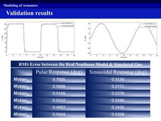
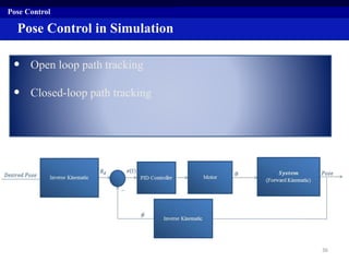
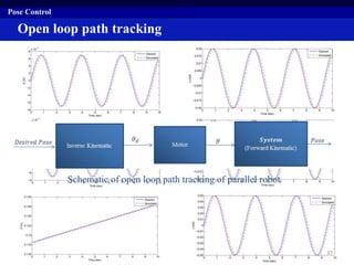
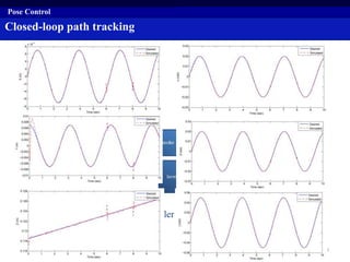
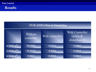
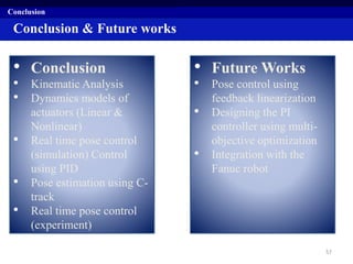
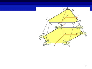
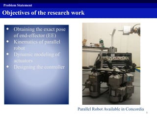
This document summarizes a research project on real time pose control of a 6-RSS parallel robot. The project involved obtaining the exact pose of the end-effector through kinematics modeling of the parallel robot, dynamic modeling of the actuators, and designing a controller for real time pose control. Kinematics were modeled using both analytical inverse and forward kinematics methods. Actuator dynamics were modeled linearly and nonlinearly, and parameters were identified using genetic algorithms and multi-objective optimization. Real time pose control was tested in simulation using open-loop and closed-loop path tracking with a PID controller.


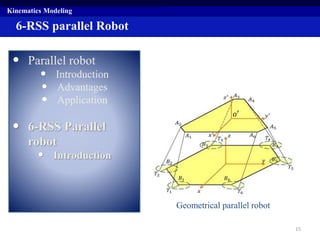
![• Parallel robot
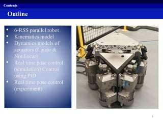
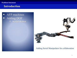
• Introduction
Parallel Robots
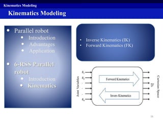
Kinematics Modeling
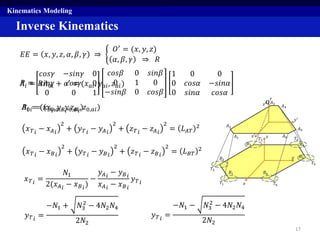
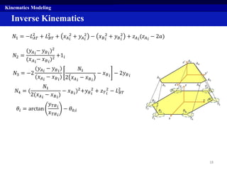
EE
Kinematic
chains
Fixed base
Link
joint
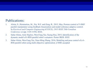
Entertainment Device for movie theater (1928) [1]
Flight simulator (1965) [1]
9](https://image.slidesharecdn.com/12e3fef6-70b3-4d40-8774-6bf7156ab76d-170105024516/85/Complete-2-9-320.jpg)
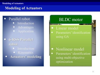
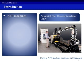
![• Parallel robot
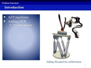
• Introduction
• Application
[4]
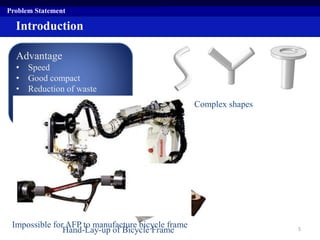
Parallel Robots
Kinematics Modeling
[2]
[1]
[3]](https://image.slidesharecdn.com/12e3fef6-70b3-4d40-8774-6bf7156ab76d-170105024516/85/Complete-2-10-320.jpg)
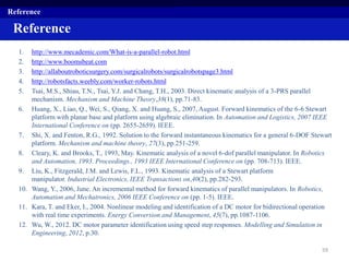
![Literature Review
• Kinematics
• Analytical Methods
Literature Review
• Tsai et al 3-DOF [5]
• Huang et al. 6-DOF [6]
• Shi et al. 6-DOF [7]
General Stewart Platform [6] 11](https://image.slidesharecdn.com/12e3fef6-70b3-4d40-8774-6bf7156ab76d-170105024516/85/Complete-2-11-320.jpg)
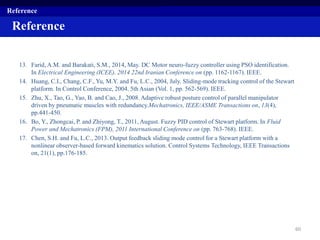
![Literature Review
• Kinematics
• Analytical Methods
• Numerical Methods
Literature Review
• Cleary et al. 6-DOF [8]
• Liu et al. 6-DOF [9]
• Wang 6-DOF [10]
General Stewart Platform [10] 12](https://image.slidesharecdn.com/12e3fef6-70b3-4d40-8774-6bf7156ab76d-170105024516/85/Complete-2-12-320.jpg)
![Literature Review
• Kinematics
• Analytical examples
• Numerical examples
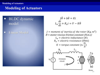
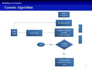
• Identification of
BLDC motor
Literature Review
• Kara et al. RLS [11]
• Wu et al. Tylor expansion theorem
[12]
• Farid et al. PSO [13]
13](https://image.slidesharecdn.com/12e3fef6-70b3-4d40-8774-6bf7156ab76d-170105024516/85/Complete-2-13-320.jpg)
![Literature Review
• Kinematics
• Analytical examples
• Numerical examples
• Identification of
BLDC motor
• Control the pose of
EE
Literature Review
• Huang et al. Sliding mode control 6-
DOF [14]
• Zhu et al. ARC 3-DOF [15]
• Bo et al. Control algorithm
based on fuzzy logic and PID control
3-DOF [16]
14](https://image.slidesharecdn.com/12e3fef6-70b3-4d40-8774-6bf7156ab76d-170105024516/85/Complete-2-14-320.jpg)