This document describes research on precise autonomous orbit control for spacecraft in low Earth orbit. It presents two main approaches: 1) further developing existing orbit control methods from an autonomous perspective, and 2) formally defining the problem of autonomous absolute orbit control as a virtual formation with one reference spacecraft affected only by Earth's gravity. The research includes developing analytical and numerical control algorithms, simulating their performance, and implementing them for an in-flight demonstration on the PRISMA mission which successfully performed autonomous orbit keeping in 2011.

1. Precise Autonomous Orbit Control in
Low Earth Orbit: from Design to
Flight Validation
Sergio De Florio
Submitted in the fulfillment of the requirements for the
Degree of Doctor of Philosophy
Division of Aerospace Sciences
School of Engineering
University of Glasgow
c
Sergio De Florio, May 2013

2. Abstract
The main purpose of this research is the analysis, development and implementation of a precise
autonomous orbit control system for a spacecraft in low Earth orbit. This thesis work represents
a step forward in the theoretical formalization and implementation of an on-board orbit main-tenance
system. Two main approaches are identified for the realization of an on-board orbit
control system. The first is the reconsideration and further development of state-of-the-art orbit
control methods from the perspective of autonomy. A step forward is then taken in the direc-tion
of the definition of a general and rigorous formalization of the autonomous orbit control
problem. The problem of the autonomous absolute orbit control is considered as a specific case
of two spacecraft in formation in which one, the reference, is virtual and affected only by the
Earth’s gravitational field. A new parametrization, the relative Earth-Fixed elements, analogous
to the relative orbital elements used for formation control, is introduced to describe the relative
motion of the real and reference sub-satellite points on the Earth surface.
An extensive discussion is dedicated to the reference orbit selection and generation process
and the analysis of the free motion of a spacecraft in low Earth orbit. The reference orbit defines
the spacecraft’s nominal trajectory designed to satisfy the mission requirements. The actual
orbit is kept within certain bounds defined with respect to the reference orbit. The generation
process of the reference orbit is dealt in detail as it is the fundamental starting point of the
orbit control chain. The free motion analysis is essential to understand the orbit perturbation
environment which causes the deviation of the actual from the nominal trajectory. The use
of the precise orbit determination data of the missions PRISMA and TerraSAR-X guarantee
the reliability of the results of this analysis and the understanding of the orbit’s perturbation
environments at an altitude of 700 and 500 km. This study helps the definition of a proper
control strategy.
The control algorithms developed in the thesis can be divided into the two broad categories of
analytical and numerical. An analytical algorithm for the maintenance of a repeat-track orbit is
developed from the state-of-the-art methods and new analytical formulations for the reference
orbit acquisition under different constraints and requirements are presented. The virtual for-mation
method for the absolute orbit control is formalized by means of the relative Earth-fixed
elements described previously. The state-space representation is used for the mathematical for-mulation
of the problem. A linear and a quadratic optimal regulators, based on this model, are
designed for the in-plane and out-of-plane absolute orbit control.
Numerical simulations are performed for the validation of the control methods. The test
platform includes a very accurate orbit propagator, the flight software and allows the simulation
of actuators and navigation errors. The simulation results are evaluated from a performance
and operational point of view in order to formulate a first conclusion about the advantages and
disadvantages of the different control techniques. The main differences between the considered
i

3. analytical and numerical control methods are outlined.
The practical implementation of a precise autonomous orbit control system for a spacecraft in
low Earth orbit is then described in detail. The on-board guidance, navigation and control soft-ware
development, implementation and testing of the PRISMA mission, to which the author
of this thesis contributed, is described. The attention is focused on the technological aspects
implied by the realization of the autonomous orbit control system tested in-flight with the au-tonomous
orbit keeping experiment on PRISMA. Among the several innovative aspects of the
flight software development, some space is dedicated to the advanced software validation and
testing realized on the formation flying test-bed at DLR, the German Aerospace Center, which
played a fundamental role in the realization of the PRISMA mission and its experiments.
Finally, the flight results of the autonomous orbit keeping experiment on the PRISMA mis-sion,
a fundamental milestone of this research work, are presented. This in-flight experiment
took place in the summer of 2011 and demonstrated the capability of autonomous precise abso-lute
orbit control using the analytical control method developed in this thesis.
ii

4. Contents
Abstract i
Acknowledgments xiii
Author’s Declaration xiv
Nomenclature xv
Symbols . . . . . . . . . . . . . . . . . . . . . . . . . . . . . . . . . . . . . . . . . xv
Greek Symbols . . . . . . . . . . . . . . . . . . . . . . . . . . . . . . . . . . . . . xvii
Indices . . . . . . . . . . . . . . . . . . . . . . . . . . . . . . . . . . . . . . . . . . xvii
Acronyms . . . . . . . . . . . . . . . . . . . . . . . . . . . . . . . . . . . . . . . . xix
Publications xxi
Journal Papers . . . . . . . . . . . . . . . . . . . . . . . . . . . . . . . . . . . . . . xxi
Conference Papers . . . . . . . . . . . . . . . . . . . . . . . . . . . . . . . . . . . xxi
Technical Documentation . . . . . . . . . . . . . . . . . . . . . . . . . . . . . . . . xxiii
1. Introduction 1
1.1. Absolute Orbit Control . . . . . . . . . . . . . . . . . . . . . . . . . . . . . . 1
1.2. Precise Autonomous Absolute Orbit Control . . . . . . . . . . . . . . . . . . . 3
1.2.1. Potential Advantages and Costs Reduction . . . . . . . . . . . . . . . 4
1.2.2. In-flight Demonstrations . . . . . . . . . . . . . . . . . . . . . . . . . 5
1.3. Ground-based vs Autonomous Orbit Control . . . . . . . . . . . . . . . . . . . 7
1.3.1. Mission Features Enabled by a Precise Orbit Control . . . . . . . . . . 7
1.3.2. Systems Comparison . . . . . . . . . . . . . . . . . . . . . . . . . . . 8
1.4. The PRISMA Mission . . . . . . . . . . . . . . . . . . . . . . . . . . . . . . 11
1.4.1. The AOK Experiment . . . . . . . . . . . . . . . . . . . . . . . . . . 14
1.5. The TerraSAR-X/TanDEM-X Missions . . . . . . . . . . . . . . . . . . . . . 14
1.6. Contributions of this Research . . . . . . . . . . . . . . . . . . . . . . . . . . 17
1.6.1. Theory . . . . . . . . . . . . . . . . . . . . . . . . . . . . . . . . . . 17
1.6.2. Transfer of Technologies from Ground to On-board Computer . . . . . 18
1.7. Thesis Outline . . . . . . . . . . . . . . . . . . . . . . . . . . . . . . . . . . . 19
2. Parametrizations 22
2.1. Overview . . . . . . . . . . . . . . . . . . . . . . . . . . . . . . . . . . . . . 22
iii

5. 2.2. Operational Parameters . . . . . . . . . . . . . . . . . . . . . . . . . . . . . . 23
2.2.1. Phase Difference . . . . . . . . . . . . . . . . . . . . . . . . . . . . . 23
2.2.2. Local Time Deviation . . . . . . . . . . . . . . . . . . . . . . . . . . 25
2.2.3. Altitude Deviation at Latitude . . . . . . . . . . . . . . . . . . . . . . 25
2.2.4. In Orbit Position Deviation . . . . . . . . . . . . . . . . . . . . . . . . 25
2.3. Virtual Formation Parametrization . . . . . . . . . . . . . . . . . . . . . . . . 26
2.3.1. Relative Orbital Elements . . . . . . . . . . . . . . . . . . . . . . . . 26
2.3.2. Relative Earth-fixed elements . . . . . . . . . . . . . . . . . . . . . . 27
3. Reference Orbit and Free Motion Analysis 31
3.1. Reference Orbit Selection . . . . . . . . . . . . . . . . . . . . . . . . . . . . . 31
3.1.1. Altitude Requirements . . . . . . . . . . . . . . . . . . . . . . . . . . 32
3.1.2. Local Time Requirements . . . . . . . . . . . . . . . . . . . . . . . . 33
3.1.3. Phasing Requirements . . . . . . . . . . . . . . . . . . . . . . . . . . 34
3.1.4. Coverage Requirements . . . . . . . . . . . . . . . . . . . . . . . . . 35
3.2. Reference Orbit Generation . . . . . . . . . . . . . . . . . . . . . . . . . . . . 35
3.2.1. Reference Orbit Propagation Model . . . . . . . . . . . . . . . . . . . 36
3.2.2. Accuracy Requirements of the Reference Orbit’s Initial State . . . . . . 40
3.3. Free Motion Analysis . . . . . . . . . . . . . . . . . . . . . . . . . . . . . . . 42
3.3.1. Free Motion of the MANGO Satellite . . . . . . . . . . . . . . . . . . 43
3.3.2. Free Motion of the TerraSAR-X Satellite . . . . . . . . . . . . . . . . 45
4. Control Methods 49
4.1. Analytical Control of Phase Difference . . . . . . . . . . . . . . . . . . . . . . 49
4.1.1. Control Concept . . . . . . . . . . . . . . . . . . . . . . . . . . . . . 50
4.1.2. Basic Orbit Keeping Strategy . . . . . . . . . . . . . . . . . . . . . . 50
4.1.3. Reference Orbit Acquisition . . . . . . . . . . . . . . . . . . . . . . . 52
4.1.4. On-board Atmospheric Drag Estimation . . . . . . . . . . . . . . . . . 55
4.2. Virtual Formation Model . . . . . . . . . . . . . . . . . . . . . . . . . . . . . 57
4.2.1. Linear Dynamic Model . . . . . . . . . . . . . . . . . . . . . . . . . . 57
4.2.2. Reduced Model . . . . . . . . . . . . . . . . . . . . . . . . . . . . . . 58
4.2.3. Characteristic Polynomial . . . . . . . . . . . . . . . . . . . . . . . . 59
4.2.4. Model Validation . . . . . . . . . . . . . . . . . . . . . . . . . . . . . 60
4.3. Virtual Formation Control . . . . . . . . . . . . . . . . . . . . . . . . . . . . 62
4.3.1. Linear Control . . . . . . . . . . . . . . . . . . . . . . . . . . . . . . 62
4.3.2. LQR Control . . . . . . . . . . . . . . . . . . . . . . . . . . . . . . . 66
4.3.3. Discrete Control . . . . . . . . . . . . . . . . . . . . . . . . . . . . . 67
5. Numerical Simulations 69
5.1. Simulation Parameters . . . . . . . . . . . . . . . . . . . . . . . . . . . . . . 69
5.2. In-Plane Orbit Control . . . . . . . . . . . . . . . . . . . . . . . . . . . . . . 71
5.2.1. Ideal Simulation Scenario . . . . . . . . . . . . . . . . . . . . . . . . 71
5.2.2. Realistic Simulation Scenario . . . . . . . . . . . . . . . . . . . . . . 73
5.3. In-Plane/Out-of-Plane Orbit Control . . . . . . . . . . . . . . . . . . . . . . . 77
iv

6. 5.4. Discussion . . . . . . . . . . . . . . . . . . . . . . . . . . . . . . . . . . . . . 79
6. On-board Orbit Control System Architecture 80
6.1. Software Design . . . . . . . . . . . . . . . . . . . . . . . . . . . . . . . . . . 80
6.1.1. Model-based Design Approach . . . . . . . . . . . . . . . . . . . . . . 80
6.1.2. Design Strategy . . . . . . . . . . . . . . . . . . . . . . . . . . . . . . 81
6.1.3. System Architecture . . . . . . . . . . . . . . . . . . . . . . . . . . . 81
6.1.4. Guidance, Navigation and Control Application Cores . . . . . . . . . . 82
6.2. Guidance, Navigation and Control Software Architecture . . . . . . . . . . . . 83
6.2.1. Top-level Architectural Design . . . . . . . . . . . . . . . . . . . . . . 83
6.2.2. Subsystems Implementation . . . . . . . . . . . . . . . . . . . . . . . 85
6.3. Autonomous Orbit Keeping Software Module . . . . . . . . . . . . . . . . . . 86
6.3.1. Top-level Architectural Design . . . . . . . . . . . . . . . . . . . . . . 86
6.3.2. Basic Logic of the AOK Controller . . . . . . . . . . . . . . . . . . . 88
6.4. Software Development and Testing Environment . . . . . . . . . . . . . . . . 91
6.4.1. Software Tests . . . . . . . . . . . . . . . . . . . . . . . . . . . . . . 93
6.4.2. Heap and Stack Tests . . . . . . . . . . . . . . . . . . . . . . . . . . . 95
6.4.3. Max-Path Tests . . . . . . . . . . . . . . . . . . . . . . . . . . . . . . 95
7. The Precise Autonomous Orbit Keeping Experiment on the PRISMA Mis-sion
100
7.1. The AOK In-Flight Experiment . . . . . . . . . . . . . . . . . . . . . . . . . . 101
7.1.1. Experiment Requirements . . . . . . . . . . . . . . . . . . . . . . . . 101
7.1.2. Reference Orbit . . . . . . . . . . . . . . . . . . . . . . . . . . . . . . 101
7.1.3. Sequence of Events . . . . . . . . . . . . . . . . . . . . . . . . . . . . 103
7.1.4. Commissioning and RO Acquisition Phases . . . . . . . . . . . . . . . 105
7.1.5. Control Tuning Phase . . . . . . . . . . . . . . . . . . . . . . . . . . . 107
7.1.6. Fine Control Phase - On-ground Generated Reference Orbit . . . . . . 108
7.1.7. Fine Control Phase - On-board Generated Reference Orbit . . . . . . . 110
7.1.8. Overall AOK Experiment Review . . . . . . . . . . . . . . . . . . . . 111
8. Conclusions 114
8.1. Discussion . . . . . . . . . . . . . . . . . . . . . . . . . . . . . . . . . . . . . 114
8.1.1. A Qualitative Cost Analysis . . . . . . . . . . . . . . . . . . . . . . . 114
8.1.2. Achievements of this Research . . . . . . . . . . . . . . . . . . . . . . 116
8.2. Future Work . . . . . . . . . . . . . . . . . . . . . . . . . . . . . . . . . . . . 118
A. Linearized Orbit Model 120
A.1. Model Matrices . . . . . . . . . . . . . . . . . . . . . . . . . . . . . . . . . . 120
A.1.1. Gravity Field . . . . . . . . . . . . . . . . . . . . . . . . . . . . . . . 120
A.1.2. Atmospheric Drag . . . . . . . . . . . . . . . . . . . . . . . . . . . . 121
A.1.3. Control Matrix . . . . . . . . . . . . . . . . . . . . . . . . . . . . . . 121
A.2. Characteristic Polynomial . . . . . . . . . . . . . . . . . . . . . . . . . . . . . 122
A.2.1. Near Circular Orbits . . . . . . . . . . . . . . . . . . . . . . . . . . . 122
v

7. A.2.2. Near Circular Orbits and no Drag . . . . . . . . . . . . . . . . . . . . 122
A.3. Transfer Function . . . . . . . . . . . . . . . . . . . . . . . . . . . . . . . . . 122
B. Navigation Accuracy in Numerical Simulations 124
C. Numerical Simulations of Combined Autonomous Absolute and Relative
Orbit Control 126
C.1. SAFE Closed-Form Analytical Control . . . . . . . . . . . . . . . . . . . . . . 127
C.2. Combination of the AOK and SAFE Analytical Controllers . . . . . . . . . . . 128
C.2.1. AOK Absolute Orbit Control . . . . . . . . . . . . . . . . . . . . . . . 128
C.2.2. SAFE Relative Control . . . . . . . . . . . . . . . . . . . . . . . . . . 129
C.3. Combination of Linear and SAFE Controllers . . . . . . . . . . . . . . . . . . 132
C.3.1. Linear Absolute Orbit Control . . . . . . . . . . . . . . . . . . . . . . 132
C.3.2. SAFE Relative Control . . . . . . . . . . . . . . . . . . . . . . . . . . 133
D. AOK Experiment Appendix 136
D.1. Orbit Perturbation Forces Environment . . . . . . . . . . . . . . . . . . . . . . 136
D.2. DVS Camera Activities . . . . . . . . . . . . . . . . . . . . . . . . . . . . . . 136
D.3. The PRISMA Formation During the AOK Experiment . . . . . . . . . . . . . 139
D.3.1. TANGO’s Navigation . . . . . . . . . . . . . . . . . . . . . . . . . . . 139
D.3.2. MANGO - TANGO Relative Motion . . . . . . . . . . . . . . . . . . 140
Bibliography 144
vi

8. List of Figures
1.1. Major Earth observation satellites in orbit or in planning (from [81]) . . . . . . 2
1.2. Orbit control process . . . . . . . . . . . . . . . . . . . . . . . . . . . . . . . 3
1.3. MANGO (a) and TANGO (b) spacecraft . . . . . . . . . . . . . . . . . . . . . 13
1.4. TerraSAR-X . . . . . . . . . . . . . . . . . . . . . . . . . . . . . . . . . . . . 15
1.5. TerraSAR-X and TanDEM-X in formation . . . . . . . . . . . . . . . . . . . . 16
2.1. Geometry of the relative Earth-fixed elements . . . . . . . . . . . . . . . . . . 28
2.2. Detail of Earth-fixed reference frame (a) and transformation from orbital to
Earth-fixed reference frame (b,c) . . . . . . . . . . . . . . . . . . . . . . . . . 28
3.1. Reference orbit selection process . . . . . . . . . . . . . . . . . . . . . . . . . 31
3.2. Reference orbit generation process . . . . . . . . . . . . . . . . . . . . . . . . 35
3.3. Difference between TANGO’s actual (POD) and propagated orbital elements . 37
3.4. MANGO’s ROE (Actual-RO) . . . . . . . . . . . . . . . . . . . . . . . . . . . 38
3.5. MANGO’s REFE at the ascending node (Actual-RO) . . . . . . . . . . . . . . 38
3.6. MANGO’s δL at the ascending node (Actual-RO) - Details . . . . . . . . . . 39
3.7. MANGO’s δL' at the ascending node (Actual-RO) - Details . . . . . . . . . . 39
3.8. MANGO’s δh at the ascending node (Actual-RO) - Details . . . . . . . . . . . 40
3.9. MANGO’s ROE (POD-RO) . . . . . . . . . . . . . . . . . . . . . . . . . . . 41
3.10. MANGO’s REFE (POD-RO) . . . . . . . . . . . . . . . . . . . . . . . . . . . 41
3.11. Free motion . . . . . . . . . . . . . . . . . . . . . . . . . . . . . . . . . . . . 42
3.12. TANGO’s ROE (POD-RO) - Propagator calibration . . . . . . . . . . . . . . . 44
3.13. MANGO’s in-plane ROE (Propagated-RO) . . . . . . . . . . . . . . . . . . . 44
3.14. MANGO’s out-of-plane ROE (Propagated-RO) . . . . . . . . . . . . . . . . . 45
3.15. MANGO’s REFE at the ascending node (Propagated-RO) . . . . . . . . . . . . 45
3.16. TSX’s ROE (POD-RO) - Propagator calibration . . . . . . . . . . . . . . . . . 46
3.17. TSX’s in-plane ROE (Propagated-RO) . . . . . . . . . . . . . . . . . . . . . . 47
3.18. TSX’s out-of-plane ROE (Propagated-RO) . . . . . . . . . . . . . . . . . . . . 47
3.19. TSX’s REFE at the ascending node (Propagated-RO) . . . . . . . . . . . . . . 48
4.1. Orbit regulator . . . . . . . . . . . . . . . . . . . . . . . . . . . . . . . . . . 49
4.2. Maneuver with estimated da/dt . . . . . . . . . . . . . . . . . . . . . . . . . 51
4.3. Smooth and timed RO acquisition from positive LAN deviation values . . . . . 53
4.4. Timed RO acquisition from negative LAN deviation values . . . . . . . . . . . 55
4.5. On-board estimation process of da/dt . . . . . . . . . . . . . . . . . . . . . . 56
4.6. TANGO’s real (POD) and propagated orbital elements with respect to the RO . 61
vii

9. 4.7. Poles computed with the RO states . . . . . . . . . . . . . . . . . . . . . . . . 62
4.8. REFE computed in u(t) and at the ascending node . . . . . . . . . . . . . . . . 68
4.9. Region of stability as mapped from the continuous to the discrete domain . . . 68
5.1. ROE (in-plane control) . . . . . . . . . . . . . . . . . . . . . . . . . . . . . . 71
5.2. REFE (in-plane control) . . . . . . . . . . . . . . . . . . . . . . . . . . . . . 72
5.3. Commanded and executed orbital maneuvers . . . . . . . . . . . . . . . . . . 73
5.4. ROE (in-plane control) . . . . . . . . . . . . . . . . . . . . . . . . . . . . . . 74
5.5. REFE (in-plane control) . . . . . . . . . . . . . . . . . . . . . . . . . . . . . 74
5.6. Commanded and executed orbital maneuvers . . . . . . . . . . . . . . . . . . 75
5.7. Mapping of continuous to discrete poles with the Tustin discretization method . 76
5.8. ROE (in-plane and out-of-plane control) . . . . . . . . . . . . . . . . . . . . . 77
5.9. REFE (in-plane and out-of-plane control) . . . . . . . . . . . . . . . . . . . . 78
5.10. Commanded and executed orbital maneuvers . . . . . . . . . . . . . . . . . . 78
6.1. Internal structure of an application component [128] . . . . . . . . . . . . . . . 82
6.2. Simplified scheme of the software architecture . . . . . . . . . . . . . . . . . . 84
6.3. Simulink subsystems implementing the BSW, ORB and GNC application cores 85
6.4. Inner structure of the ORB application core . . . . . . . . . . . . . . . . . . . 86
6.5. Simplified scheme of the software architecture . . . . . . . . . . . . . . . . . . 89
6.6. Simplified scheme of the software architecture . . . . . . . . . . . . . . . . . . 90
6.7. Software development and validation at DLR (a, c) and SSC (b, d) [131] . . . . 92
6.8. Software development and validation environments at DLR and SSC . . . . . . 96
6.9. Software development and validation environments at DLR and SSC . . . . . . 96
6.10. Software development and validation environments at DLR and SSC . . . . . . 97
7.1. Remote sensing activity planning (left). Volcanoes Etna and Stromboli as im-aged
on 10th of August (top) and on 15th of August (bottom) 2011. Images
courtesy of OHB Sweden. . . . . . . . . . . . . . . . . . . . . . . . . . . . . 101
7.2. AOK experiment sequence of events . . . . . . . . . . . . . . . . . . . . . . . 104
7.3. Semi-major axis deviation (top), LAN deviation (middle), computed orbitalma-neuvers
(bottom) . . . . . . . . . . . . . . . . . . . . . . . . . . . . . . . . . 106
7.4. Semi-major axis deviation and on-board estimation accuracy (top). Orbital ma-neuvers
(bottom) . . . . . . . . . . . . . . . . . . . . . . . . . . . . . . . . . 106
7.5. Semi-major axis deviation (top), LAN deviation (middle), maneuvers (bottom) 108
7.6. Semi-major axis deviation (top), LAN deviation (middle), maneuvers (bottom) 109
7.7. Semi-major axis deviation (top), LAN deviation (middle), maneuvers (bottom) 110
7.8. Semi-major axis deviation (top), LAN deviation (middle), maneuvers (bottom) 111
7.9. Accuracy of the on-board estimated position in RTN . . . . . . . . . . . . . . 113
7.10. Accuracy of the on-board estimation of the semi-major axis . . . . . . . . . . . 113
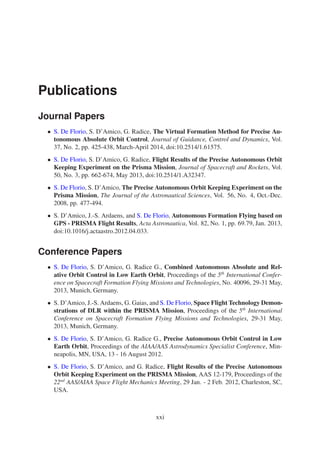
8.1. Ground-based vs on-board orbit control systems cost . . . . . . . . . . . . . . 115
B.1. Accuracy of the on-board estimated position in RTN . . . . . . . . . . . . . . 124
B.2. Accuracy of the on-board estimated orbital elements . . . . . . . . . . . . . . 125
viii

10. C.1. Relative orbital elements (AOK) . . . . . . . . . . . . . . . . . . . . . . . . . 128
C.2. Relative Earth-fixed elements and executed orbital maneuvers - AOK . . . . . . 129
C.3. Relative orbital elements AFC-AOK . . . . . . . . . . . . . . . . . . . . . . . 130
C.4. Relative Earth-fixed elements AFC-AOK . . . . . . . . . . . . . . . . . . . . 130
C.5. Executed formation control maneuvers AFC-AOK . . . . . . . . . . . . . . . . 131
C.6. Earth-fixed baseline TSX-TDX . . . . . . . . . . . . . . . . . . . . . . . . . . 132
C.7. Relative orbital elements - Linear regulator . . . . . . . . . . . . . . . . . . . 133
C.8. Relative Earth-fixed elements and executed orbital maneuvers - Linear regulator 133
C.9. Relative orbital elements SAFE-Linear . . . . . . . . . . . . . . . . . . . . . . 134
C.10.Relative Earth-fixed elements AFC-Linear . . . . . . . . . . . . . . . . . . . . 134
C.11.Executed formation control maneuvers AFC-Linear . . . . . . . . . . . . . . . 135
D.1. Solar flux indices F10.7 and Kp from January 2000 to September 2011 . . . . . 137
D.2. Solar flux indices F10.7 and Kp during the AOK experiment . . . . . . . . . . 137
D.3. South Europe from 4th to 12th of August. Images courtesy of OHB Sweden. . . 138
D.4. TANGO’s GPS antennas switch (top) and GOD measurement update status
(bottom) . . . . . . . . . . . . . . . . . . . . . . . . . . . . . . . . . . . . . . 140
D.5. Relative position MANGO - TANGO in the RTN orbital frame during the ac-quisition
phase of the initial relative state for AOK experiment . . . . . . . . . 141
D.6. Relative orbital elements MANGO - TANGO during the acquisition phase of
the initial relative state for AOK experiment . . . . . . . . . . . . . . . . . . . 141
D.7. Relative eccentricity and inclination vectors MANGO - TANGO during the ac-quisition
phase of the initial relative state for AOK experiment . . . . . . . . . 142
D.8. Relative positionMANGO - TANGO in the RTN orbital frame during the AOK
experiment . . . . . . . . . . . . . . . . . . . . . . . . . . . . . . . . . . . . 142
ix

11. List of Tables
1.1. Overview of mission parameters for some remote sensing satellites . . . . . . . 1
1.2. Costs Reduction . . . . . . . . . . . . . . . . . . . . . . . . . . . . . . . . . . 4
1.3. Autonomous absolute orbit contol in-flight demonstrations . . . . . . . . . . . 5
1.4. Enabled Mission Features . . . . . . . . . . . . . . . . . . . . . . . . . . . . . 8
1.5. Comparison between ground-based and on-board orbit control systems . . . . . 9
1.6. PRISMA GNC experiments . . . . . . . . . . . . . . . . . . . . . . . . . . . 12
1.7. PRISMA sensor/actuator experiments . . . . . . . . . . . . . . . . . . . . . . 12
3.1. Orbit specification in terms of nominal mean orbital elements . . . . . . . . . . 32
3.2. Control specifications . . . . . . . . . . . . . . . . . . . . . . . . . . . . . . . 36
3.3. PRISMA spacecraft physical properties . . . . . . . . . . . . . . . . . . . . . 36
3.4. Propagation parameters . . . . . . . . . . . . . . . . . . . . . . . . . . . . . . 37
3.5. Initial state - POD state on 20-06-2011 at 06:00:00 UTC . . . . . . . . . . . . 37
3.6. On-board navigation error . . . . . . . . . . . . . . . . . . . . . . . . . . . . 40
3.7. Influence of orbit perturbation forces on the orbital elements . . . . . . . . . . 43
3.8. Physical properties of the TerraSAR-X spacecraft . . . . . . . . . . . . . . . . 46
3.9. Propagation initial state . . . . . . . . . . . . . . . . . . . . . . . . . . . . . . 46
4.1. Analytic expressions of the poles . . . . . . . . . . . . . . . . . . . . . . . . . 59
4.2. Propagation parameters . . . . . . . . . . . . . . . . . . . . . . . . . . . . . . 60
4.3. Poles computed in the initial state . . . . . . . . . . . . . . . . . . . . . . . . 61
4.4. Gain constraints . . . . . . . . . . . . . . . . . . . . . . . . . . . . . . . . . . 64
5.1. Propagation parameters . . . . . . . . . . . . . . . . . . . . . . . . . . . . . . 70
5.2. Navigation and actuators accuracy . . . . . . . . . . . . . . . . . . . . . . . . 70
5.3. Regulators design parameters . . . . . . . . . . . . . . . . . . . . . . . . . . . 72
5.4. Control performance and maneuver budget with in-plane control . . . . . . . . 73
5.5. Control performance and maneuver budget with in-plane control . . . . . . . . 75
5.6. Poles . . . . . . . . . . . . . . . . . . . . . . . . . . . . . . . . . . . . . . . . 76
5.7. Control performance and maneuver budget with in-plane and out-of-plane control 78
6.1. Application components for GNC software . . . . . . . . . . . . . . . . . . . 83
6.2. AOK software module input . . . . . . . . . . . . . . . . . . . . . . . . . . . 87
6.3. AOK software module output . . . . . . . . . . . . . . . . . . . . . . . . . . . 87
6.4. Structure of AOK status byte . . . . . . . . . . . . . . . . . . . . . . . . . . . 88
6.5. AOK maneuvers computation . . . . . . . . . . . . . . . . . . . . . . . . . . . 91
6.6. LEON3 board and host laptop PC features . . . . . . . . . . . . . . . . . . . . 94
x

12. 6.7. Execution times and CPU loads . . . . . . . . . . . . . . . . . . . . . . . . . 98
7.1. AOK experiment requirements . . . . . . . . . . . . . . . . . . . . . . . . . . 102
7.2. AOK experiment sequence of events . . . . . . . . . . . . . . . . . . . . . . . 103
7.3. AOK controller settings during the fine control phase . . . . . . . . . . . . . . 108
7.4. Most significant control statistics . . . . . . . . . . . . . . . . . . . . . . . . . 109
7.5. Most significant control statistics . . . . . . . . . . . . . . . . . . . . . . . . . 110
7.6. Maneuver v budget . . . . . . . . . . . . . . . . . . . . . . . . . . . . . . . 112
B.1. Navigation error - Position and velocity in RTN . . . . . . . . . . . . . . . . . 124
B.2. Navigation error - Orbital elements . . . . . . . . . . . . . . . . . . . . . . . . 125
C.1. Control performance and maneuver budget of AOK control . . . . . . . . . . . 129
C.2. Control performance and maneuver budget of AFC relative control . . . . . . . 131
C.3. Control performance and maneuver budget of in-plane linear control . . . . . . 132
C.4. Control performance and maneuver budget of AFC relative control . . . . . . . 135
D.1. Requested and actual MANGO - TANGO relative initial state for the AOK ex-periment
. . . . . . . . . . . . . . . . . . . . . . . . . . . . . . . . . . . . . . 140
xi

13. to Paride, may he rest in peace
Beethoven Op. 31 No. 2
xii

14. Acknowledgments
I would like to expressmy gratitude tomy supervisors Gianmarco Radice and Simone D’Amico.
Gianmarco gave me the trust and freedom I needed to accomplish this research. Simone is
the scientist who taught me the art of flight dynamics in which he is a real master. I owe
special thanks also to Oliver Montenbruck from whom I learned the importance of realising
concretely ideas conceived during research. Thanks to Jean-Sebastian and Gabriella for their
invaluable support during the AOK experiment operations and to the PRISMA mission design
and operations team in Sweden.
Thanks to
My parents and my sister for their constant support and patience
My grandmother who guards my roots in Milano
Giangi for the excellent dinners and Whisky
Gianni and Paride who visited me in Glasgow and joined us in the Burns night
Elisa, Ettore, Fabrizio, Giuseppe, Lorenzo, Luca, Marcel.la, Matteo, Michele, Miguel, Paola,
Saika, Serena, Yago and Yamagen for everything in the daily life in München
My theatre and athletics groups because they are also families
Dieter, my athletics trainer, for telling me that rests are as important as trainings
Claire, Filiep, Franz, Markus, Matthias, Paul and Stefan for the running trainings together
Thomas for showing me new paths in music
Carlo because the future is in space
Claudia so far but so close
Paola, Maura, Daniela and Fabio for their determined daily commitment
Guido, Lamberto and Giovanni who are like brothers
Eli for she exists
Sergio De Florio
xiii

15. Author’s Declaration
I hereby declare that this submission is my own work and that, to the best of my knowledge and
belief, it contains no material previously published or written by another person nor material
which to a substantial extent has been accepted for the award of any other degree or diploma of
the university or other institute of higher learning, except where due acknowledgment has been
made in the text.
Glasgow, Scotland, June 26, 2013, Sergio De Florio
xiv

16. Nomenclature
Symbols
a = semi-major axis [m]
aij = element ij of matrix A
A = spacecraft reference area [m2]
A = dynamic model matrix [s-1]
bij = element ij of matrix B
B = ballistic coefficient of the spacecraft [kg/m2]
B = control matrix [-]
c = cost [e]
cij = element ij of matrix C
C = output matrix [-]
CD = drag coefficient [-]
da/dt = decay rate of the semi-major axis [m/s]
dt = time difference [s]
e = eccentricity [-]
e = eccentricity vector [-]
ec = orbit control accuracy [m]
ed = dynamic model uncertainties [m]
ej = eccentricity vector component [-]
eM = maneuvers error [m]
eN = navigation error [m]
F10.7 = solar radio flux index [sfu = 10-22 W m-2 Hz-1]
gj = gain
G = gain matrix
Gd = disturbance gain matrix
Kp = geomagnetic activity index [-]
i = inclination [rad]
ij = inclination vector component [rad]
JA = Jacobian of matrix A
J2 = geopotential second-order zonal coefficient [-]
m = spacecraft mass [kg]
M = mean anomaly [rad]
n = mean motion [rad/s]
nN = nodal frequency [1/s]
xv

17. RE = Earth’s equatorial radius [m]
sj = characteristic root
t = time [s]
tc = time required for reference orbit acquisition [s]
te = exploitation time [s]
tsmooth = time required for smooth reference orbit acquisition [s]
T = maneuver cycle [s]
T = coordinates transformation matrix [-]
Tdu = maneuver duty cycle [d]
TE = mean period of solar day [s]
TN = nodal period [s]
TSu = Sun period [s]
u = argument of latitude [rad]
u = constant value of argument of latitude [rad]
v = spacecraft velocity [m/s]
δa = relative semi-major axis [-]
aAN = difference between real and reference semi-major axis at the ascending node [m]
ac = maneuver semi-major axis increment [m]
δe = relative eccentricity vector amplitude [-]
δej = relative eccentricity vector component [-]
δ̥ = relative Earth-fixed elements vector [-]
δh = normalized altitude difference [-]
h = altitude difference [m]
δi = relative inclination vector amplitude [rad]
δij = relative inclination vector component [rad]
δκ = relative orbital elements vector
δLj = phase difference vector component [m]
L = phase difference [m]
LAN = phase difference at the ascending node [m]
LMAX = LAN control window [m]
δr = normalized relative position vector [-]
δrj = component of normalized relative position vector[-]
δu = relative argument of latitude [rad]
δv = normalized relative velocity vector [-]
δvj = component of normalized relative velocity vector[-]
vj = impulsive maneuver velocity increment component [m/s]
vMAX = largest value allowed for a maneuver [m/s]
R− = set of negative real numbers
R+ = set of positive real numbers
Z = set of integer numbers
Z+ = set of positive integer numbers
xvi

18. Greek Symbols
ǫ = normalized relative orbital elements vector [m]
η = normalized altitude [-]
φ = relative perigee [rad]
ϕ = latitude [rad]
κ = mean orbital elements vector
κo = osculating orbital elements vector
λ = longitude [rad]
μ = Earth’s gravitational coefficient [m3/s2]
ω = argument of periapsis [rad]
ωE = Earth rotation rate [rad/s]
= right ascension of the ascending node [rad]
˙
= secular rotation of the line of nodes [rad/s]
ρ = atmospheric density [kg/m3]
τ = time constraint for reference orbit acquisitions [s]
θ = relative ascending node [rad]
ξ = thrusters execution error [%]
Indices
Subscripts
c = closed-loop
CMD = commanded
d = disturbance
D = discrete
du = duty cycle
E = Earth
EXE = executed
g = gravity
i = implementation
m = maneuver
n = navigation
N = cross-track
onb = on-board
ong = on-ground
OPS = operations
p = performance
r = reduced
R = reference orbit
R = radial
sy = Sun-synchronous
xvii

19. sth = smoothed
T = along-track
TOT = total
Superscripts
T = vector transpose
xviii

20. Acronyms
ACC Accelerometer
AFC Autonomous formation control
AMS Asynchronous monotonic scheduler
AOC Autonomous orbit control
AOCS Attitude and orbit control system
AOK Autonomous Orbit Keeping
BSW Basic software
CDTI Spanish Centre for the Development of Industrial Technology
CNES French Space Agency
COTS Commercial off the shelf
CPU Central processing unit
DEM Digital elevation model
DLR German aerospace center
DTU Technical University of Denmark
DVS Digital video system
ECI Earth-centred inertial
EF Earth-fixed
EGSE Electrical Ground Support Equipment
EM Engineering model
FDIR Failure detection isolation and recovery
FF Formation flying
FFRF Formation flying radio frequency sensors
FM Flight model
GIF GPS interface
GNC Guidance, navigation and control
GOD GPS-based Orbit Determination
GOP GPS-based Orbit Prediction
GS Ground station
GSOC German space operations center
IRF Institute of Space Physics
ISL Inter-satellite-link
LEO Low Earth Orbit
LPO Longitudinal phase of the orbit
MBD Model-based design
MM Magnetometer
OBC On-board computer
OCK Orbit Control Kit
ONB On-board
PC Personal computer
POD Precise Orbit Determination
RAMSES Rocket And Multi Satellite EGSE System
xix

21. REFE Relative Earth-Fixed elements
RCC RTEMS cross-compilation
RMS Root mean square
RO Reference Orbit
ROE Relative orbital elements
RTEMS Real-time executive for multiprocessor systems
RTOS Real time operating system
RTU Remote terminal unit
RTW Real time workshop
SAFE Spaceborne autonomous formation flying experiment
SAR Synthetic aperture radar
SCA star camera
SCET Spacecraft Elapsed Time
S/C Spacecraft
SEU Singular event upset
SNSB Swedish National Space Board
SRP Solar radiation pressure
SS Sun sensor
SSC Swedish space corporation
SSP Sub-satellite point
SSTL Surrey Satellite Technology Limited
S/W Software
TAFF TanDEM-X autonomous formation flying
TAN Time at ascending node
TBC To be confirmed
TC Telecommand
TDX TanDEM-X
THR Thrusters
TM Telemetry
TSX TerraSAR-X
TTTC Time-tagged-telecommand
UV Ultra Violet
VBS Vision based sensor
xx

22. Publications
Journal Papers
• S. De Florio, S. D’Amico, G. Radice, The Virtual Formation Method for Precise Au-tonomous
Absolute Orbit Control, Journal of Guidance, Control and Dynamics, Vol.
37, No. 2, pp. 425-438, March-April 2014, doi:10.2514/1.61575.
• S. De Florio, S. D’Amico, G. Radice, Flight Results of the Precise Autonomous Orbit
Keeping Experiment on the Prisma Mission, Journal of Spacecraft and Rockets, Vol.
50, No. 3, pp. 662-674, May 2013, doi:10.2514/1.A32347.
• S. De Florio, S. D’Amico, The Precise Autonomous Orbit Keeping Experiment on the
Prisma Mission, The Journal of the Astronautical Sciences, Vol. 56, No. 4, Oct.-Dec.
2008, pp. 477-494.
• S. D’Amico, J.-S. Ardaens, and S. De Florio, Autonomous Formation Flying based on
GPS - PRISMA Flight Results, Acta Astronautica, Vol. 82, No. 1, pp. 69.79, Jan. 2013,
doi:10.1016/j.actaastro.2012.04.033.
Conference Papers
• S. De Florio, S. D’Amico, G. Radice G., Combined Autonomous Absolute and Rel-ative
Orbit Control in Low Earth Orbit, Proceedings of the 5th International Confer-ence
on Spacecraft Formation Flying Missions and Technologies, No. 40096, 29-31May,
2013, Munich, Germany.
• S. D’Amico, J.-S. Ardaens, G. Gaias, and S. De Florio, Space Flight Technology Demon-strations
of DLR within the PRISMA Mission, Proceedings of the 5th International
Conference on Spacecraft Formation Flying Missions and Technologies, 29-31 May,
2013, Munich, Germany.
• S. De Florio, S. D’Amico, G. Radice G., Precise Autonomous Orbit Control in Low
Earth Orbit, Proceedings of the AIAA/AAS Astrodynamics Specialist Conference, Min-neapolis,
MN, USA, 13 - 16 August 2012.
• S. De Florio, S. D’Amico, and G. Radice, Flight Results of the Precise Autonomous
Orbit Keeping Experiment on the PRISMAMission, AAS 12-179, Proceedings of the
22nd AAS/AIAA Space Flight Mechanics Meeting, 29 Jan. - 2 Feb. 2012, Charleston, SC,
USA.
xxi

23. • S. De Florio, S. D’Amico, G. Radice G., Operations Concept of the Precise Autonomous
Orbit Keeping Experiment on the PRISMA Mission, Proceedings of the 8th IAA Sym-posium
on Small Satellites for Earth Observation, 4-8 April 2011, Berlin.
• S. De Florio, S. D’Amico and J.S. Ardaens, Autonomous Navigation and Control of
Formation Fliyng Spacecraft on the PRISMA Mission, IAC-10.C1.5.12, Proceedings
of the 61st International Astronautical Congress, 27 Sep - 1 Oct 2010, Prague, CZ. (2010).
• S. D’Amico, J.S. Ardaens, S. De Florio, O. Montenbruck, S. Persson, R. Noteborn
R., GPS-Based Spaceborne Autonomous Formation Flying Experiment (SAFE) on
PRIS-MA: Initial Commissioning, Proceedings of the AIAA/AAS Astrodynamics Spe-cialist
Conference, 2-5 August 2010, Toronto, Canada.
• S. D’Amico, J.-S. Ardaens and S. De Florio, Autonomous Formation Flying based
on GPS - PRISMA Flight Results, Proceedings of the 6th International Workshop on
Satellite Constellations and Formation Flying, IWSCFF, November 1-3, 2010, Howard
International House, Taipei, Taiwan
• S. De Florio, S. D’Amico, Optimal Autonomous Orbit Control of Remote Sensing
Spacecraft, Proceedings of the 19th AAS/AIAA Space Flight Mechanics Meeting, 8-12
Feb 2009, Savannah, USA.
• S. De Florio, E. Gill, S. D’Amico, Performance Comparison of Microprocessors for
Space-based Navigation Applications, Proceedings of the 7th IAA Symposium on Small
Satellite for Earth Observation, 4-8 May 2009, Berlin, Germany.
• S. D’Amico, S. De Florio, R. Larsson, M. Nylund, Autonomous Formation Keeping
and Reconfiguration for Remote Sensing Spacecraft, Proceedings of the 21st Interna-tional
Symposium on Space Flight Dynamics, 28 Sep. - 2 Oct. 2009, Toulouse, France.
• S. De Florio, S. D’Amico,M. Garcia-Fernandez, The Precise Autonomous Orbit Keep-ing
Experiment on the PRISMA Formation Flying Mission, AAS 08-212, Proceed-ings
of the 18th AAS/AIAA Space Flight Mechanics Meeting, 28-31 Jan. 2008, Galveston,
Texas, USA.
• S. De Florio, Reduction of the Response Time of Earth Observation Satellite Con-stellations
using Inter-satellite Links, AIAA-2008-3281, Proceedings of the SpaceOps
Conference, 12-16 May 2008, Heidelberg, Germany.
• S. D’Amico, J.-S. Ardaens, S. De Florio, O. Montenbruck, Autonomous Formation
Flying - TanDEM-X, PRISMA and Beyond, Proceedings of the 5th InternationalWork-shop
on Satellite Constellations and Formation Flying, 2-4 July 08, Evpatoria, Crimea,
Ukraine.
• S. D’Amico, S. De Florio, J. S. Ardaens, T. Yamamoto, Offline and Hardware-in-the-loop
Validation of the GPS-based Real-Time Navigation System for the PRISMA
xxii

24. Formation Flying Mission, Proceedings of the 3rd International Symposium on Forma-tion
Flying, Missions and Technology, 23-25 April 2008, ESA/ESTEC, Noordwijk, The
Netherlands.
Technical Documentation
• S. De Florio, Flight Results of the Precise Autonomous Orbit Keeping Experiment on
the PRISMA Mission, PRISMA-DLR-OPS-56, 2011, DLR/GSOC, Deutsches Zentrum
für Luft und Raumfahrt, Oberpfaffenhofen, Germany.
• S. De Florio, Operation Concept of the Precise Autonomous Orbit Keeping Experi-ment
on the PRISMA Mission, PRISMA-DLR-OPS-55, 2011, DLR/GSOC, Deutsches
Zentrum für Luft und Raumfahrt, Oberpfaffenhofen, Germany.
• S. De Florio, S. D’Amico, Collision Risk Assessment for Co-orbiting Spacecraft,
DEOS-DLR-TN-02, 2011, DLR/GSOC, Deutsches Zentrum für Luft und Raumfahrt,
Oberpfaffenhofen, Germany.
• S. De Florio, DLR’s Experiment Control Center for the PRISMA Mission Interface
Control Document, PRISMA-DLR-OPS-52, DLR/GSOC, Deutsches Zentrum für Luft
und Raumfahrt, Oberpfaffenhofen, Germany.
• S. De Florio, S. D’Amico, Real-Time Satellite Laboratory Tests of DLR’s Flight
Software: Third SATLAB Campaign (v. 6.2.0), PRISMA-DLR-TST-45, DLR/GSOC,
Deutsches Zentrum für Luft und Raumfahrt, Oberpfaffenhofen, Germany.
• S. De Florio, S. D’Amico, DLR’s Satellite Laboratory Test Results for the PRISMA
Flight Software, PRISMA-DLR-TST-44, DLR/GSOC, Deutsches Zentrum für Luft und
Raumfahrt, Oberpfaffenhofen, Germany.
• S. De Florio, S. D’Amico, Comparison of Scalar and Vectorial Implementation of the
Extended Kalman Filter, PRISMA-DLR-TN-19, DLR/GSOC, Deutsches Zentrum für
Luft und Raumfahrt, Oberpfaffenhofen, Germany.
• S. De Florio, S. D’Amico, Max-Path Unit Tests of the PRISMA Flight Software,
PRISMA-DLR-TN-17, DLR/GSOC, Deutsches Zentrum für Luft und Raumfahrt, Oberp-faffenhofen,
Germany.
xxiii

25. 1. Introduction
1.1. Absolute Orbit Control
In the last two decades the development and exploitation of very high resolution optical systems
mounted on satellites in Low Earth Orbit (LEO) was a major driver for the commercialisation
of Earth observation data. The global political security situation, environmental awareness and
updated legislative frameworks are pushing for the realization of new high resolution remote
sensing missions. The European Global Monitoring for Environment and Security (GMES)
programme now renamed Copernicus is a major example of this trend. Fig. 1.1 [81] shows
a list of significant Earth observation missions in orbit or planned for the near future. These
kind of missions demand specialized orbits. Remote sensing satellites are generally placed on
so-called sun-synchronous orbits where they cross the true of date Earth equator at the ascend-ing
node at the same local time. This is necessary to ensure similar illumination conditions
when making images of the same parts of the Earth’s surface with the exploitation of different
orbits. In addition, orbits of remote sensing satellites are often designed to repeat their ground
track after a certain number of days. These are the so called phased orbits. Finally, it may
be useful to minimize or even avoid the secular motion of the argument of perigee of the or-bit.
This is again achieved by a proper choice of the orbital parameters and the resulting orbit
is called frozen. Orbits of remote sensing satellites are, in general, sun-synchronous, phased,
and frozen simultaneously. A collection of typical orbital elements and of phasing parameters
for remote sensing satellites is given in Table 1.1. The design of such orbits is based on the
required characteristics of the motion of the spacecraft with respect to the Earth surface. The
three-dimensional position of the spacecraft in an Earth-fixed (EF) frame is completely defined
by its projection on the ground track and its altitude with respect to the Earth’s surface. The
design of the orbit will thus define a nominal EF trajectory to be maintained during the entire
mission lifetime. Specific orbit control requirements can be expressed by means of constraints
Table 1.1.: Overview of mission parameters for some remote sensing satellites
Mission ERS 1 SPOT 4 Envisat 1 TerraSAR Sentinel-1
Agency ESA CNES ESA DLR ESA
Launch date July 1991 March 1998 June 2001 June 2007 2013 (TBC)
Mean altitude [km] 775 822 800 514 693
a [km] 7153 7200 7178 6786 7064
e [-] 0.001 0.001 0.025 0.0013
i [deg] 98.5 98.7 98.6 97.4 98.2
Phasing [days/orbits] 3/43 26/369 35/501 11/167 12/175
1

26. 1. Introduction
Figure 1.1.: Major Earth observation satellites in orbit or in planning (from [81])
2

27. 1. Introduction
Figure 1.2.: Orbit control process
on certain quantities, the operational parameters, which define the maximum allowed deviation
of the real from the nominal ground track and altitude of the spacecraft. The orbit control is
based on the maintenance of these operational parameters within prescribed limits which repre-sent
the dead-bands for the orbit control. The operational parameters depend on the deviation of
the orbital elements from their nominal values under the action of perturbing forces. Once the
mission requirements have been translated into orbit control margins, it is necessary to compute
the corrections to be applied to the orbital elements to keep the value of the operational param-eters
within their control windows. Fig. 1.2 shows the basic block diagram of the orbit control
process and in which chapters of this thesis the relevant topics are treated. The requirements
which determine the reference orbit (RO) can change in some cases during the course of the
mission. From the RO the nominal EF parameters to be controlled can be computed by means
of a coordinates transformation represented by block Tin in Fig. 1.2. A similar transformation
process Tout is used to obtain the actual EF parameters from the actual orbit of the spacecraft
which varies under the actions of the natural forces determining the motion of the spacecraft.
The difference between the nominal and the actual values of the EF parameters are the input
to the orbit regulator. The control actions computed by the orbit regulator are then executed
by the spacecraft’s thrusters. The feedback control scheme of Fig. 1.2 [76-80] is valid for a
ground-based or on-board orbit control system the differences being in the single blocks and in
the way in which the control process is operated.
1.2. Precise Autonomous Absolute Orbit Control
Autonomous on-board orbit control means the automatic maintenance by the spacecraft itself
of different operational parameters within their control dead-bands. Increasing the autonomy
of spacecraft is often considered an additional unnecessary risk conflicting with the optimal
planning of the payload activities. Nevertheless the exploitation of an autonomous on-board
3

28. 1. Introduction
orbit control system brings some fundamental advantages and enables some specific mission
features. The principal roadblock to introducing the autonomous orbit control technology is
simply tradition. Orbit control has always been done from the ground and new programs do not
want to risk change for what is perceived as a marginal benefit for that flight.
1.2.1. Potential Advantages and Costs Reduction
Table 1.2 [62] resumes some advantages and costs reduction resulting by the use of an au-tonomous
on-board orbit control system. The fulfilment of very strict control requirements on
different orbit parameters can be achieved in real time and with a significant reduction of flight
dynamics ground operations [62]. With a fine on-board orbit control system the spacecraft fol-lows
a fully predictable RO pattern, such that the position of the spacecraft at all future times
is known as far in advance as desirable and there is a longer planning horizon for all future
activities.
The scheduling and planning burden can thus be reduced. With a ground-based orbit control
system, planning is done as far in advance as feasible in terms of future orbit propagation. If
preliminary plans are done then an updated plan will be created several days in advance, and
final updates will be made as close to the event as possible so that the predicted positions can
be as accurate as possible. An autonomous on-board fine orbit control eliminates all of the
replanning and rescheduling process and allows these activities to be done on a convenient
business basis rather than dictated by the orbit prediction capability. Long-term planning can
be done on a time lapse basis as convenient for the user group. These plans are updated as the
needs of the users change and the detailed schedule of events is prepared in a manner convenient
for operations and dissemination [65].
This technology provides a new and unique capability in that even very simple ground equip-ment
that remains out of contact for extended periods can know where a satellite autonomously
controlled is and when they will next be within contact. This reduces the cost and complexity
of providing needed ephemeris information to the user community.
A tighter control is generally associated with additional propellant usage. For LEO satellites
the dominant in-track secular perturbation is the atmospheric drag. The requirement on the
orbit control system is to put back what drag takes out. By timing the thruster burns correctly
this negative velocity increment can be put back so as to maintain the in-track position with
Table 1.2.: Costs Reduction
Cost reduction Rationale
Operations Eliminating the need for ground-based orbit maintenance
Planning and scheduling
By knowing the precise future positions of the spacecraft (or
all of the spacecraft in a constellation)
Ephemerides transmission
The cost and complexity of transmitting spacecraft
ephemerides to various users is eliminated
Lower propellant usage The orbit is continuously maintained at its highest level
4

29. 1. Introduction
no additional propellant usage over that required to overcome the drag force. Since the orbit is
continuouslymaintained at its highest level rather than being allowed to decay and then brought
back up, the effect of drag is minimized and the required propellant usage is also minimized
[58]. By increasing the required control accuracy the number of smaller thruster firings will
increase. This provides a much finer granularity of control and has the secondary advantage of
minimizing the orbital maneuvers disturbance torque. Generally, the largest thruster firing for
a fine orbit control is a few times the minimum impulse bit of the thrusters being used. This
is, by definition, the smallest level of thrust the propulsion system can efficiently provide and,
therefore, the smallest orbital maneuvers disturbance torque. In some cases it may even be
possible to do the thruster firings while the payload is operating.
1.2.2. In-flight Demonstrations
In the last two decades different studies have been done for the autonomous orbit control of
satellites in LEO [49-64]. Some of these theoretical works were validated in the in-flight demon-strations
listed in Table 1.3. All these experiments have in common the GPS-based on-board
navigation which is nowadays the only means to obtain a continuous accurate on-board orbit
estimation and thus an accurate orbit control. The time at ascending node (TAN) and the longi-tude
of ascending node (LAN) are the parameters controlled by means of along-track velocity
increments whereas the longitudinal phase of the orbit (LPO) is controlled by means of cross-track
maneuvers. The RO is propagated using only the Earth’s gravitational field model and
this means that the orbit controller has to keep the gravitational perturbations and correct all
the others which are no-conservative forces. Indeed the gravitational perturbations do not cause
orbit decay and can be modeled precisely enough by numerical means to enable prediction of
the satellite position far into the future.
The Microcosm Inc. Orbit Control Kit (OCK) software [77] was flown the first time on the
Surrey Satellite Technology Limited (SSTL) UoSAT-12 [65] spacecraft, where it co-resides on
a customized 386 onboard computer, developed by SSTL, with their attitude determination and
control system software. The inputs for OCK are generated by the SSTL-built 12-channel L1-
code GPS receiver (SSTL model SGAR 20) with an output frequency of 1 Hz. Microcosm
Table 1.3.: Autonomous absolute orbit contol in-flight demonstrations
Year 1999 2005 2007 2011
Mission UoSAT-12 Demeter TacSat-2 PRISMA
Orbit 650 km sun-sync. 700 km sun-sync. 410 km sun-sync. 710 km sun-sync.
Exp. duration [days] 29 150 15 30
Ctrl type TAN/LPO/e LAN/TAN/e TAN LAN/TAN
Ctrl accuracy [m] 930 100 750 10
Total v [m/s] 0.0733 0.12 0.27 0.13
Propulsion Cold gas Hydrazine Hall Effect Thruster Hydrazine
Navigation GPS GPS GPS GPS
Ctrl system developer Microcosm, Inc. CNES Microcosm, Inc. DLR/SSC
Exp. = experiment, Ctrl = control, TAN = Time at Ascending Node, LAN = Longitude of Ascending Node
5

30. 1. Introduction
demonstrated in flight two different high-accuracy in-track orbit controllers and one cross-track
controller. In the implementation of the in-track controllers, the basic measurement to be con-trolled,
by means of along-track velocity increments, is the TAN i.e. the deviation from the
expected value in the crossing time from South to North of the Earth’s equator. The actual
and reference crossing times are compared for the computation of the required maneuver [58].
On-board targeting of frozen orbit conditions is used to better control the orbit average perfor-mance.
A proprietary method is used to continually move the orbit toward frozen conditions
and, once achieved, hold it there. Orbit-averaged mean elements are also calculated on board.
An analogous process to in-track control has been implemented for the cross track control. The
cross-track error is determined by comparing the longitude measured at the ascending node to
a pre-determined longitude. However, the LPO and not the inclination is controlled by means
of cross-track maneuvers. This means that any secular drift in the placement of the orbit plane
are removed over time until the desired longitudinal position and drift rate are maintained. An
updated and enhanced version of OCK was validated in-flight on TacSat-2 [66] which carried
the IGOR GPS receiver developed by Broad Reach Engineering. The goal of this experiment
was controlling autonomously the TAN and validating new functionalities of OCK. A series of
three short validation tests, lasting up to several days, were performed. These short duration
tests were followed by a fourth extended test that lasted two weeks. Similar to the experiment
on UoSat-12, OCK managed to maintain the in-track position with an accuracy of 750 m over
an extended period of time on TacSat-2, in spite of a variety of off-nominal events.
The main objective of the autonomous orbit control (AOC) experiment on Demeter [67-
71] was to control, autonomously and securely in an operational context, the TAN, the LAN
and the mean eccentricity vector of the satellite by means of along-track velocity increments.
The control algorithms used are similar to those presented in Sec. 4.1.2. The on-board orbit
determination for the experiment was based on a Thales Alenia Space TOPSTAR 3000 GPS
receiver [67]. The AOC software was installed in the GPS receiver and used the time, position,
velocity plus other indicators as supplied by the GPS receiver for its computations. Time slots
for the orbital maneuvers were defined since one of the main constraints was that AOC could
not interfere with the scientific mission operations. These time slots, consisting of one orbital
period close to a ground station pass, were defined on-ground and uploaded regularly. Only
one orbital maneuver per slot was allowed and the size of the velocity increments which could
be executed autonomously was also bounded. The ground segment made use of a RO defined
consistently with the reference parameters used by the AOC. One of the most interesting aspects
of Demeter is that the AOC systemwas used routinely after its validation and its operations were
coordinated with the scientific payload activities.
The autonomous orbit keeping (AOK) experiment on the PRISMA mission [72-75] is de-scribed
in detail in Chapter 7. The AOK experiment has demonstrated the nowadays most
accurate absolute orbit control in full autonomy and with simple operational procedures. The
guidance, navigation and control (GNC) architecture of PRISMA (Chapter 6) is structured with
orbit control softwaremodules separated fromthe navigationmodules and installed in the space-craft’s
on-board computer whereas in the Demeter satellite the control software is installed di-rectly
in the GPS receiver [67,69]. The LAN (Chapter 2) and the TAN, as for Demeter, was
controlled at the same time by means of along-track velocity increments
6

31. 1. Introduction
These in-flight experiments represent milestones in demonstrating that this technology has
now reached a sufficient level of maturity to be applied routinely in LEO missions.
1.3. Ground-based vs Autonomous Orbit Control
As explained in detail by the qualitative cost analysis of Sec. 8.1.1, by increasing the control
accuracy requirements, thus reducing the maneuver cycle, the choice of using an autonomous
orbit control system can be more convenient. The ratio between the maneuver cycle and the
maximum time between two consecutive ground station contacts is one of the most important
drivers in the choice for a ground-based or on-board orbit control system. There is indeed a
minimum value of the maneuver cycle for which an autonomous orbit control system is the
only feasible option as the latency between the ground station contacts is too large for the
exploitation of a ground-based control.
1.3.1. Mission Features Enabled by a Precise Orbit Control
Table 1.4 [62] resumes some specific mission features which are enabled by a precise orbit
control. With autonomous orbit keeping, planning and scheduling are done on a business basis,
not as astrodynamics dictates. Thus a detailed plan can be put out well in advance to allow time
for convenient distribution and potential coordination and input among the mission users. User
terminals, such as remote weather stations or bookstore computers with daily receipts, can be
delivered to the user with the entire spacecraft ephemeris already in memory. Consequently,
data can be transmitted autonomously when the satellite is overhead. Similarly, worldwide
science groups can do observation planning based on advance knowledge of where the satellite
will be and the detailed lighting and viewing conditions then. All of this provides a new level
of utility while substantially reducing the cost and complexity of providing needed ephemeris
information to the user community.
The fundamental problem with avoiding both collisions and RF interference is to know about
it as far in advance as possible. This allows coordination with other system operators and,
as discussed above, allows avoidance maneuvers to be done as fuel efficiently as possible. A
system using autonomous orbit control may choose to make the future positions of its satellites
public. This allows any other satellite users or potential users to calculate as far in advance
as possible when potential collisions or interference could occur. This provides the maximum
possible warning and permits advance coordination.
For a satellite constellation [64-50] retaining the structure at minimum cost and risk is fun-damental.
An autonomous orbit control system on-board each satellite can maintain the orbital
period such that the mean period will be the same for all satellites in the constellation over its
lifetime. This maintains all the satellites synchronized with each other and ensures that the con-stellation
structure will be fully maintained over the lifetime of the satellites without periodic
rephasing or readjustment.
The combined use of new low-power electric propulsion technologies and autonomous guid-ance,
navigation, and control techniques provides an effective way to reduce the costs of the
orbit maintenance of a satellite in LEO. The use of a suitable electric propulsion system allows
7

32. 1. Introduction
Table 1.4.: Enabled Mission Features
Feature Rationale
Mission scheduling in advance
The customer of the mission can plan data-take far
in advance and for long period of times
Mission planning in advance
The mission control team knows well in advance
when and where the spacecraft will be
Simple user terminals
User terminals with very simple ground equip-ments
for data reception have the entire spacecraft
ephemeris in advance
Collision avoidance
Space situational awareness teams have an accu-rate
information on the position of the autonomous
spacecraft at any time
Rendezvous
Rendezvous operations are simplified by a tar-get
autonomous spacecraft as its trajectory is well
known
Coverage analysis for constellations
All users know where all of the satellites are all of
the time with no comm link
Eliminate constellation rephasing
All satellites in the constellation are maintained in
phase with each other at all times
Use of electric propulsion in LEO
The reduced size of the maneuvers allows the use
of a low thrust propulsion system
Use in planetary missions
Costs are lowered due to the possibility of au-tomating
data retrieval from the surface
for significant savings on propellant mass and a consequent increase of the spacecraft lifetime
[56].
The use of a satellite with an autonomous on-board orbit control system around a planet of
the solar system to be explored (e.g. Mars) could lower the mission costs due to the possibility
of automating data retrieval from the surface [51].
1.3.2. Systems Comparison
The advantages brought by an autonomous orbit control system explained in Sec. 1.2.1 can
be afforded indeed by a ground-based control system (except of course for the reduction of
the on-ground operations costs) at the condition of a high control accuracy. A routine orbit
maintenance with an accuracy of 250 m, at an altitude of 500 km, in the directions perpendicular
to the reference ground track has been demonstrated by the TerraSAR-X mission [44,114].
Future missions like Sentinel-1 [118-121] are planned to have a control accuracy requirement
of 50 m at an altitude of 700 km. It is necessary to track the main differences, advantages and
disadvantages of the two options and identify in which cases one method is more convenient
8

33. 1. Introduction
than the other. Fig. 1.2 shows which operations of the orbit control process can be executed
on-ground or on-board. Table 1.5 resumes schematically the points of confrontation between
ground-based and on-board orbit control systems.
If the orbit control system is ground-based, the only operation executed on-board is the
thrusters activation by means of time-tagged-telecommands (TTTC) uploaded to the space-craft
during a ground station contact and the complementary activities (e.g. attitude maneuvers,
computation and correction of thruster activation times, etc.). The ground-based orbit deter-mination
process needs eventually data downloaded from the spacecraft (e.g. GPS, attitude
and maneuvers data). The value of the orbital maneuvers computed on-ground is typically the
output of an optimization process which have the availability of space environment data col-lected
on the long period, the most precise navigation data and practically no constraints on the
computational resources. The ground station contacts with the spacecraft provide navigation
and housekeeping data to the ground segment. These data are filtered and used for an orbit
determination to get the best possible knowledge of the satellite status and motion. The oper-ational
parameters are computed and handed over to the orbit control software. Inputs for the
orbit determination and controller software are also external data, consisting of up-to-date solar
flux data, Earth rotation parameters, eventual navigation payload (e.g. GPS) auxiliary data and
propulsion system information. The controller compares the predicted operational parameters
over a certain period of time with the control dead-bands and computes a time-tagged maneuver
which is uploaded to the spacecraft in the next ground station contact. The main operational
Table 1.5.: Comparison between ground-based and on-board orbit control systems
Element On-ground On-board
RO Best available
Best available if uploaded or less accu-rate
if generated on-board
Navigation (GPS) POD 10 times less accurate
Orbit perturbations Long period accurate data On-board estimation or uploaded
Computing resources Virtually unlimited Limited
Control software
Optimization process with
no hardware or time con-straints
Designed considering CPU resources
constraints
Man. computation Optimized
Including on-board navigation errors
and limited information about space
environment
GS contacts Necessary for control Verification only
Reaction time GS contacts latency time In real time
Thrusters Thrusters performance limitations
Attitude control Errors included in the computation of the maneuvers
Man. = maneuver, GS = ground station
9

34. 1. Introduction
constraint is related with the satellite visibility to the available network of ground stations. In
fact a minimum lapse of time is required for the upload of the orbital maneuver instructions to
the spacecraft and the verification that they have been correctly stored on-board. The ground
station contacts are limited due to geographic position of the station and the costs for contact
time. Only with a polar ground station a contact visibility is possible every orbit for LEO satel-lites
whereas a ground station at middle latitudes allows typically two scheduled contact per day
meaning that the satellite conditions can be checked with an interval of 12 hours. The reaction
time of the orbit control system is then commensurate to the latency time of the ground station
contacts. An adequate number of post-maneuver passes out of the normal mission schedule,
and involving ground station not pertaining to the ground segment, may be required to verify
that the maneuver has been executed correctly and that the desired effect on the operational
parameters has been obtained.
If the orbit control systemis on-board, one of the operations which can be optionally executed
on-ground is the RO generation which can be uploaded to the spacecraft in form of TTTC
during a ground station contact (Chapter 7). Other operations which are executed on-ground
to support the on-board orbit control system are the calibration of the controller’s parameters
and the atmospheric density modelling. The major limitation for the generation of the RO
on-board is due to the available computational resources of the spacecraft’s on-board computer
(OBC) which determines the quality of the orbit propagation model that can be used. The initial
state of the RO on-board propagation can be a state of the precise orbit determination (POD)
ephemerides generated on-ground or a state generated by the on-board navigation system. In the
latter case the propagation of the on-board orbit estimation error has to be considered carefully
(Sec. 3.2.2). Once the RO is available, all the operations of the control chain are executed on-board
the spacecraft. The main advantage of an on-board with respect to ground-based control
systemis that it reacts in real time to the deviations from the nominal trajectory of the spacecraft.
The ground station contacts are included in the orbit control chain only to verify that the system
is working properly and no additional contacts have to be scheduled. Some major limitations
concerning the inputs and the software have to be considered in designing an autonomous on-board
orbit maintenance system. The on-board navigation data will include an error which can
be ten times that of a ground-based POD (for a GPS-based orbit estimation process) [73]. This
error will impact on the accuracy of the computed orbital maneuver. The information about the
orbital environment is also very limited. An on-board estimation of the atmospheric drag, the
main non-gravitational perturbation in LEO, required for the computation of the maneuvers can
be done using the navigation data filtered and fitted (Sec. 4.1.4). The orbit environment data
required by the on-board orbit propagation model can be eventually updated periodically by
means of a data upload. The regulator software design has to be compliant with the constraints
dictated by the computational and data storage resources of the spacecraft’s OBC. A long period
optimization process is thus generally not available on-board.
The satellite-bus constraints regarding both control systems, concern mainly the performance
of the spacecraft’s attitude control and thrusters accuracy. The accuracy of the attitude control
system and of the on-board thrusters influence the effectiveness of the orbital maneuvers. The
location of the thrusters on-board the spacecraft determines the attitude maneuver profile re-quired
before and after an orbit control maneuver. Besides, the correct operation of certain
10

35. 1. Introduction
attitude sensors (e.g. star sensors) may impose time-slots during which the orbital maneuvers
cannot be executed. Another important operational issue is that often the science payload can-not
work during the orbital maneuvers and the orbit maintenance and payload schedules have
to be integrated together. If the control chain is ground-based the scheduling of the payload
and orbit maintenance operations can be optimized. If the orbit control system is on-board, the
eventual orbital maneuvers are input as a constraint in the scheduling problem.
1.4. The PRISMA Mission
A substantial part of this research is motivated and finds its application in the frame of the
PRISMA mission and was realized at the German Space Operations Center (GSOC) of the
German Aerospace Center (DLR). PRISMA [82-109] is a micro-satellite formation mission
created by the Swedish National Space Board (SNSB) and Swedish Space Corporation (SSC)
[168], which serves as a platform for autonomous formation flying and rendezvous of space-craft.
The formation comprises a fully maneuverable micro-satellite (MANGO) as well as a
smaller satellite (TANGO) which were successfully launched aboard a Dnepr launcher from
Yasny, Russia, on June 15th 2010 into a nominal dawn-dusk orbit at a mean altitude of 757
km, 0.004 eccentricity and 98.28◦ inclination. The PRISMA mission primary objective is to
demonstrate in-flight technology experiments related to autonomous formation flying, homing
and rendezvous scenarios, precision close range 3D proximity operations, soft and smooth final
approach and recede maneuvers, as well as to test instruments and unit developments related to
formation flying. Key sensors and actuators comprise a GPS receiver system, two vision based
sensors (VBS), two formation flying radio frequency sensors (FFRF), and a hydrazine mono-propellant
thruster system (THR). These support and enable the demonstration of autonomous
spacecraft formation flying, homing, and rendezvous scenarios, as well as close-range proxim-ity
operations. The experiments can be divided in Guidance, Navigation and Control (GNC)
experiments and sensor/actuator experiments. The GNC experiment sets consist of closed loop
orbit control experiments conducted by SSC and the project partners which are the German
Aerospace Center (DLR/GSOC), the French Space Agency (CNES) in partnership with the
Spanish Centre for the Development of Industrial Technology (CDTI), the Technical University
of Denmark (DTU), ECAPS (a subsidiary company to SSC), Nanospace (a subsidiary company
to SSC), Techno Systems (TSD) and Institute of Space Physics (IRF) in Kiruna. Table 1.6 col-lects
the GNC primary and secondary objectives and the involvement of the different project
partners. Table 1.7 resumes the sensor/actuator primary and secondary experiments and the in-volvement
of the different project partners. In addition to the GPS-based absolute and relative
navigation system, which is the baseline navigation sensor for the on-board GNC functionali-ties,
DLR contributes two dedicated orbit control experiments. The primary experiment, named
Spaceborne Autonomous Formation Flying Experiment (SAFE) [92,143], was executed suc-cessfully
in two parts, the first one in 2010 and the second one in 2011. SAFE implements
autonomous formation keeping and reconfiguration for typical separations below 1 km based
on GPS navigation. The secondary experiment of the DLR’s contributions to PRISMA is AOK
which implements the autonomous absolute orbit keeping of a single spacecraft. The MANGO
spacecraft (Fig. 1.3.a) has a wet mass of 150 kg and a size of 80 x 83 x 130 cm in launch config-
11

36. 1. Introduction
Table 1.6.: PRISMA GNC experiments
Primary GNC related tests
Type of control Distance [m] Sensor Prime
Autonomous formation flying 20-5000 GPS SSC
Proximity operations [101] 5-100 VBS/GPS SSC
Collision avoidance and autonomous rendezvous 10-100000 VBS/GPS SSC
Autonomous formation control (SAFE) [92,143] 50-1000 GPS DLR
RF-based FF and forced RF-based motion [100,109] 20-5000 FFRF CNES
Secondary GNC related tests
Autonomous Orbit Keeping (AOK) of a single spacecraft [72-75] GPS DLR
uration, has a three-axis, reaction-wheel based attitude control and three-axis delta-v capability.
The GNC sensors equipment comprises two three-axes magnetometers, one pyramid sun acqui-sition
sensors and five sun-presence sensors, five single-axis angular-rate sensors, five single-axis
accelerometers, two star-tracker camera heads for inertial pointing, two GPS receivers, two
vision-based sensors and two formation flying radio frequency sensors. Three magnetic torque
rods, four reaction wheels and six thrusters are the actuators employed. Electrical power for the
operation of the spacecraft bus and payload is provided by two deployable solar panels deliver-ing
a maximum of 300 W. In contrast to the highly maneuverable MANGO satellite, TANGO
(Fig. 1.3.b) is a passive and much simpler spacecraft, with a mass of 40 kg at a size of 80 x 80 x
31 cm with a coarse three-axes attitude control based on magnetometers, sun sensors, and GPS
receivers (similar toMANGO), with three magnetic torque rods as actuators and no orbit control
capability. The nominal attitude profile for TANGO will be sun or zenith pointing. Required
power is produced by one body-mounted solar panel providing a maximum of 90 W. The com-munication
between the ground segment and the TANGO spacecraft is only provided through
MANGO acting as a relay and making use of a MANGO-TANGO inter-satellite link (ISL) in
the ultra-high-frequency band with a data rate of 19.2 kbps. DLR/GSOC, besides designing
and conducting his own experiments, has assumed responsibility for providing the GPS-based
Table 1.7.: PRISMA sensor/actuator experiments
Primary Hardware Related Tests
Experiment Prime
Flight demo of GPS Phoenix receiver DLR
Flight demo of HPGP motor [82] SSC
Flight demo of micro-thrusters motor [99] Nanospace
Validation of RF sensor (FFRF) CNES
Validation of Vision Based Sensor (VBS) DTU
Secondary hardware related tests
Flight demo of a digital video system Techno System
Flight demo of a MEMS-based particle mass spectrometer IRF
12

37. 1. Introduction
Figure 1.3.: MANGO (a) and TANGO (b) spacecraft
navigation functionality which comprises the provision of Phoenix GPS receivers [103-105],
the GPS based on-board navigation system for absolute/relative orbit determination and the
ground-based POD [83-85]. In fact the on-board navigation system includes two Phoenix-S
GPS receivers and the real-time orbit estimation software with an absolute (relative) position
accuracy capability of 2 (0.2) m (3D, RMS) in nominal conditions under the provision of suffi-cient
GPS data. The ground-based POD provides absolute (relative) position accuracies better
than 0.1 (0.05) m (3D, RMS). The GPS measurements collected on TANGO are transferred
to MANGO via the ISL. The navigation system provides absolute position and velocity of the
participating spacecraft to be used by the MANGO GNC system as well as the other PRISMA
experiments. The GPS system provides also timing information for on-board synchronization.
The physical architecture of the GPS system is identical on MANGO and TANGO. For redun-dancy,
two Phoenix-S GPS receivers are available, which are connected to two GPS antennas
via a coaxial switch. The dual antenna system provides increased flexibility for handling non-zenith
pointing attitudes and antennas may be selected by ground command or autonomously
on-board. Only one receiver will be active at any time. Continuous orbit information is im-portant
for autonomous on-board GNC applications. As a consequence, orbit prediction is a
mandatory function of the navigation system and provides continuous absolute and relative po-sition
and velocity information of the co-orbiting satellites. Furthermore the navigation system
provides an accuracy measure indicating the expected quality of the orbit results.
13

38. 1. Introduction
1.4.1. The AOK Experiment
The AOK experiment on the PRISMA mission was executed successfully from the 18th of July
to the 16th of August 2011 and has demonstrated the capability of autonomous absolute or-bit
control with an unprecedented accuracy. The main scientific goal of the experiment was
to demonstrate the accuracy, robustness and reliability of an autonomous GPS-based on-board
orbit control for its possible routine exploitation in future scientific missions. The main differ-ences
with respect to similar experiments conducted in the past (Sec. 1.2.2) are the extremely
tight requirements on control accuracy and the full autonomy also enhanced by the possibil-ity
of on-board RO propagation. The AOK controller adopts a guidance law for the orbital
Longitude of the Ascending Node (LAN) and implements the analytical feedback control algo-rithm
presented in Sec. 4.1. Using GPS-based absolute navigation data, the on-board controller
commanded thruster activations in the orbital frame to autonomously control the orbit within a
predefined window. The main performance requirement of the experiment was a control accu-racy
of the osculating ascending node of 10 m (1 σ standard deviation) with a maneuver velocity
increment-decrement (v) available budget of 0.5 m/s. The AOK software was first developed
and tested using the offline and hardware-in-the-loop test facilities at DLR (Chapter 6). After
the integration in the PRISMA flight-software, AOK was thoroughly tested at OHB Sweden
by means of the Real-Time Satellite Laboratory (SATLAB), a hardware-in-the-loop test facil-ity
[87]. The experiment operations were executed at the DLR’s PRISMA experiment control
centre while the mission was operated at DLR/GSOC. A commissioning phase of 4 days was
required to verify that the control software was working properly in all its functionalities. Dur-ing
this phase MANGO flew in free motion as the controller was in open-loop and the orbital
maneuvers were computed on-board but not executed. The closed-loop phase of 26 days in-cluded
RO acquisition, controller tuning and fine control phases. In the last four days of the
experiment the possibility of exploiting a RO generated on-board the spacecraft was tested in
closed-loop. The 10 m control accuracy requirement was fulfilled. The mean value of the lon-gitude
of ascending node deviation was -3.6 m with a standard deviation of 9.5 m during the
fine control phase. The on-board controller demonstrated also to be very accurate in computing
and executing RO acquisitions. The total v spent during the entire experiment was 0.1347
m/s corresponding to 27% of the allocated maneuvers budget. The mean maneuver cycle was
11 hours with a standard deviation of 8.3 hours. The position accuracy available on-board was
about 2 m (1 σ) during the entire experiment whereas the accuracy of the on-board estimation of
the semi-major axis was 4 m (1 σ) as it comes from a combination of the accuracies of position
and velocity.
1.5. The TerraSAR-X/TanDEM-X Missions
TerraSAR-X/TanDEM-X represents the typical remote sensing mission which could take ad-vantage
of a precise autonomous orbit control system. TerraSAR-X (TSX) [110-117] is a Ger-man
Earth-observation satellite realized in a public-private partnership between the German
Federal Ministry of Education and Research (BMBF), DLR and EADS Astrium GmbH. The
primary goal of the TSX mission (Fig. 1.4) is the provision of high-resolution Synthetic Aper-
14

39. 1. Introduction
Figure 1.4.: TerraSAR-X
ture Radar (SAR) data to both science and commercial users. Its primary payload is an X-band
radar sensor with a range of different modes of operation, allowing it to record images with
different swath widths, resolutions and polarisations. TSX thus offers space-based observation
capabilities that were previously unavailable. The objective of the mission is to provide value-added
SAR data in the X-band, for research and development purposes as well as scientific and
commercial applications. The successful launch of TSX on 15th June 2007 from the Russian
Baikonur Cosmodrome in Kazakhstan marked the start of a campaign to map the Earth at an
unprecedented level of accuracy. The aim is to create new, high-quality radar images of the
Earth’s surface. The satellite has a size of 4.88 x 2.4 m, a mass of 1230 kg and flies in a 514
km sun-synchronous dusk-dawn orbit with an inclination of 97.4◦ and an 11 day repeat period.
Using its active radar antenna, TSX it is able to produce image data with a resolution of down
to 1 m, regardless of weather conditions, cloud cover or absence of daylight. TSX [171] has
been fully operational since 7 January 2008. The radar beam can be electronically tilted within
a range of 20 to 60 degrees perpendicular to the flight direction, without having to move the
satellite itself. This allows the radar to zoom in on many more ground targets from the satel-lite’s
orbit than would be possible using a non-steerable radar. In order to support the spacecraft
AOCS and to enable high-precision orbit reconstruction the satellite bus is equipped with a sin-gle
frequency GPS receiver and the secondary payload features a dual frequency GPS receiver.
Due to the objectives of the interferometric campaigns the satellite has to comply to tight orbit
control requirements, which are formulated in the form of a toroidal tube with a radius of 250 m
around a pre-flight determined reference trajectory [32]. To minimize both the interruption of
SAR data takes and the total amount of thruster firings, the maintenance of semi-major axis and
eccentricity is simultaneously achieved by a single maneuver at an optimized location [44,110].
15

40. 1. Introduction
Figure 1.5.: TerraSAR-X and TanDEM-X in formation
The orbit maintenance maneuvers are executed by the mono-propellant (Hydrazine) 4 x 1 N
propulsion system.
TanDEM-X (TDX) was built to form the first configurable SAR interferometer employing
formation flying with TSX. The main objective of the common TerraSAR-X/TanDEM-X mis-sion
(Fig. 1.5) is to generate a global digital elevation model (DEM) with unprecedented accu-racy
as the basis for a wide range of scientific research as well as for commercial DEM produc-tion.
TDX [172] was launched on 21th June 2010 and acquired an initial formation with 20 km
along-track separation for commissioning purposes roughly one month later. The close forma-tion
flight with separations of a few hundred meters was finally established in October 2010.
TSX/TDX is the first operational mission requiring a post-facto baseline reconstruction with an
accuracy of 1 mm. The TDX/TSX relative orbit control concept is based on the relative eccen-tricity/
inclination vector separation method [143,144]. TDX is equipped with an Autonomous
Formation Flying (TAFF) system [111,112] developed at DLR/GSOC. The implementation of
autonomous formation flying functionalities on the TDX spacecraft is considered to be a key
driver for a more efficient use of the available on-board resources. The objective of TAFF is to
enable a simple and robust formation control in order to ease the on-ground operations. TAFF
16

41. 1. Introduction
is implemented as part as the attitude and orbit control system on-board TDX and is intended
to take over the in-plane formation keeping activities throughout the mission, with a control
accuracy of a few meters. A short closed-loop test campaign of TAFF, during which all the
functionalities of the autonomous software could be successfully tested, was performed at the
end of March 2011.
1.6. Contributions of this Research
The main research topic of this thesis is the autonomous orbit control of a single spacecraft. A
fundamental achievement is the rigorous formalization of the absolute orbit control problem as
a special case of formation keeping. For this reason this work can found its collocation in the
research dedicated to the spacecraft formation flying [143]. The AOK and SAFE experiments
on the PRISMA mission are two complementary in-flight realistic demonstrations of a complete
GNC system respectively for autonomous absolute and relative orbit control in a LEO orbit.
1.6.1. Theory
The first step of this research is the reconsideration of state-of-the-art orbit control methods
[3,42-48] from the perspective of autonomy. Starting from an analytical algorithm for the main-tenance
of a repeat-track orbit, the control chain of Fig. 1.2 is developed and implemented under
the assumption of the availability of a GPS-based on-board navigation. An algorithm is devel-oped
for the on-board estimation, by means of navigation data, of the semi-major axis decay
caused by the atmospheric drag. New analytical formulations for the RO acquisition under
different constraints and requirements are developed.
Particular emphasis is given to the analysis of the RO generation process which can be
ground-based or on-board. The main achievement of this analysis is the definition of constraints
on the minimal accuracy of the orbit model used and of the initial state for the propagation. An
extensive study of the orbit perturbation environment in LEO is carried on. The results of this
study have the added value, with respect to similar analyses performed in the past, of the avail-ability
of a large amount of POD data from the missions PRISMA and TerraSAR-X which have
near circular orbit at respectively 700 and 500 km. These POD data have an accuracy better
than 10 cm (1 σ) and have also been used for the calibration of the orbit models used for all the
numerical simulations performed during this research work.
The state-of-the-art orbit control methods are based on a formalization of the problem which
is dependent on the particular mission and its orbit maintenance requirements. A step forward
is then taken in the direction of the definition of a general and rigorous formalization of the
autonomous orbit control problem and the exploration of new control methods. The problem
of the autonomous absolute orbit control is considered as a specific case of two spacecraft in
formation in which one, the reference, is virtual and affected only by the Earth’s gravitational
field. A new parametrization, the relative Earth-Fixed elements (REFE), analogous to the rela-tive
orbital elements (ROE) [137,159], is introduced to describe the relative motion of the real
and reference sub-satellite points on the Earth surface. The REFE allow the general formal-ization
of the absolute orbit control requirements which are usually expressed through specific
17

42. 1. Introduction
Earth-fixed operational parameters such as altitude deviation, phase difference, etc. [3]. A di-rect
mapping between REFE and ROE enables the direct translation of absolute into relative
orbit control requirements. By means of this new formalization, the deviation between the ac-tual
and the reference nominal orbit [32] can be defined in an Earth-fixed coordinate system
analogous to the orbital frame [4]. This approach allows moreover the straightforward use of
modern control theory techniques for orbit control. A linear and a quadratic optimal regulators
are designed and compared, by means of numerical simulations, with the analytical algorithms.
The goal is to show a method rather than some specific simulation results. The particular abso-lute
and relative orbit control problem with its requirements can be formalized using every time
the same parametrization given by the REFE and the ROE.
1.6.2. Transfer of Technologies from Ground to On-board
Computer
The innovation and originality of this thesis derives also from the design and practical imple-mentation
of the control chain of Fig. 1.2 in the frame of the PRISMA mission. This research
work has led to the full development, testing and validation of the autonomous absolute orbit
control flight code embedded in the OBC of theMANGO spacecraft of the PRISMA technology
demonstration. The design and validation of the GPS-based flight software throughout its com-plete
development process, up to the spacecraft launch, is described. The innovative approach
of model-based software design (MBD) is addressed. The MBD allows the implementation and
execution of the GNC software on different platforms in a fully consistent manner. The GNC
system was first tested as a standalone unit in a dedicated software development environment
at DLR [170] and later validated after its full integration into the PRISMA spacecraft on-board
computer. This allows first to develop the software simulations off-line on a PC and then to
reproduce them consistently as real-time and hardware-in-the-loop tests during the validation
phase. In the off-line tests, the flight software is stimulated through different sources of GPS
data with an increasing level of realism. The complete application is then ported to a Real-Time
Executive forMultiprocessor Systems (RTEMS) environment in the LEON3 PRISMA on-board
computer by means of MATLAB/Simulink Real Time Workshop. Overall the test and valida-tion
process shows the compliance of the navigation and control software to the challenging
requirements of the PRISMA mission in terms of functionality, data interface, GNC accuracy,
on-board memory and CPU load.
The flight data of the AOK [72-75] experiment on the PRISMA mission [167] are displayed
and commented. The main scientific goal of the experiment, successfully executed in the sum-mer
of 2011, was to demonstrate the accuracy, robustness and reliability of an autonomous
GPS-based on-board orbit control for its possible routine exploitation in future scientific mis-sions.
Autonomous precise orbit maintenance, RO acquisition and on-board RO generation
have been successfully demonstrated in orbit.
18

43. 1. Introduction
1.7. Thesis Outline
This thesis is structured in seven chapters complemented by an appendix section. Referring to
Fig. 1.2, after an extensive theoretical dissertation of the different blocks composing the orbit
control chain, the attention is focused on the practical implementation, validation and testing of
the considered autonomous orbit control methods.
The thesis starts with an extended general discussion about orbit control requirements and
the state of the art of its implementation. The attention is focused on the advantages brought
by the exploitation of an autonomous orbit maintenance system in terms of costs reduction and
enabled mission features. A statistical comparison between ground-based and on-board orbit
control is not possible because only few autonomous orbit control in-flight experiments have
been performed so far. Nevertheless a qualitative discussion and cost analysis can be made
based on the available literature and on the author’s practical experience. A fundamental state-ment
is that a major driver to the development of on-board autonomous orbit control is the
increasing accuracy demand due to the steady development and exploitation of very high res-olution
optical and synthetic aperture radars systems in the last two decades. A description of
two missions, PRISMA and TerraSAR-X/TanDEM-X, is also given in the introduction since
a substantial part of this research is motivated and finds its application in the frame of those
projects. The PRISMA mission gave the possibility to perform an autonomous orbit keep-ing
experiment which validated successfully one of the orbit control methods proposed in this
thesis. The TerraSAR-X/TanDEM-X formation represents the typical remote sensing mission
which can take advantage of a precise autonomous orbit control system.
After the introduction, the thesis proceeds explaining, in Chapter 2, the parametrizations
used, the basic mathematical means on which the different orbit control methods proposed are
based. Two main approaches are identified for the realization of an on-board orbit control sys-tem.
The first is the reconsideration and further development of state-of-the-art orbit control
methods from the perspective of autonomy. A step forward is then taken in the direction of
the definition of a general and rigorous formalization of the autonomous orbit control problem.
The problem of the autonomous absolute orbit control is considered as a specific case of two
spacecraft in formation in which one, the reference, is virtual and affected only by the Earth’s
gravitational field. A new parametrization, the relative Earth-Fixed elements (REFE), analo-gous
to the relative orbital elements used for formation control, is introduced to describe the
relative motion of the real and reference sub-satellite points on the Earth surface. The relative
Earth-Fixed elements allow the general formalization of the absolute orbit control requirements
which are usually expressed, with the first approach, through specific Earth-fixed operational
parameters (e.g. altitude deviation, phase difference, etc.).
An extensive discussion is dedicated in Chapter 3 to the RO selection and generation process
and the analysis of the free motion of a spacecraft in low Earth orbit. The RO defines the
spacecraft’s nominal trajectory designed to satisfy the mission requirements. The actual orbit
is kept within certain bounds defined with respect to the RO. The RO selection process based
on the mission requirements is briefly described as well as the typical orbits used for remote
sensing. The link between the operational parameters and the requirements is explained. The
generation process of the RO is dealt in detail as it is the fundamental starting point of the
19

44. 1. Introduction
orbit control chain. The free motion analysis is essential to understand the orbit perturbation
environment which causes the deviation of the actual from the nominal trajectory. The use
of the precise orbit determination data of the missions PRISMA and TerraSAR-X guarantee
the reliability of the results of this analysis and the understanding of the orbit’s perturbation
environments at an altitude of 700 and 500 km. This study helps the definition of a proper
control strategy. The conclusions drawn in this chapter about the RO generation process are also
based on the experience gained with the realization of the AOK in-flight experiment described
in Chapter 7.
The control algorithms, explained in Chapter 4, can be divided into the two broad categories
of analytical and numerical. An analytical algorithm for the maintenance of a repeat-track or-bit
is developed from the state-of-the-art methods and implemented under the assumption of
the availability of a GPS-based on-board navigation. A complementary algorithm for the on-board
estimation of the semi-major axis decay caused by the atmospheric drag is developed.
New analytical formulations for the RO acquisition under different constraints and require-ments
are presented. The virtual formation method for the absolute orbit control is formalized
by means of the relative Earth-fixed elements described previously in the chapter dedicated to
the parametrization. The state-space representation is used for the mathematical formulation
of the problem. The system to be controlled is described by means of a linear dynamic model
including the J2 zonal coefficient of the Earth’s gravitational field and the atmospheric drag per-turbation
force. A linear and a quadratic optimal regulators, based on this model, are designed
for the in-plane and out-of-plane absolute orbit control. Among the control methods presented
in this chapter, only the analytical algorithm was validated in-flight with the AOK experiment
on the PRISMA mission because it had a most advanced implementation status at the moment
of its selection.
The entire Chapter 5 deals with the results of the numerical simulations performed for the
validation of the control methods explained in Chapter 4. The high degree of realism of the
simulations’ results is guaranteed by a calibration of the orbit propagator model by means of
the comparison between the propagated and the actual orbit data given by the POD process of
the PRISMA and TerraSAR-X missions. The mission parameters of these two formations are
also used as simulation scenarios. The test platform includes a very accurate orbit propagator,
the flight software and allows the simulation of actuators and navigation errors. The simulation
results are evaluated from a performance and operational point of view in order to formulate a
first conclusion about the advantages and disadvantages of the different control techniques. The
main differences between the considered analytical and numerical control methods are outlined.
Once the theory has been explained extensively, the practical implementation of a precise
autonomous orbit control system for a spacecraft in low Earth orbit is described in detail in
Chapter 6. The on-board guidance, navigation and control software development, implemen-tation
and testing of the PRISMA mission, to which the author of this thesis contributed, is
described. The attention is focused on the technological aspects implied by the realization of
the autonomous orbit control system tested in-flight with the autonomous orbit keeping experi-ment
on PRISMA. The development of the control system is driven by a compromise between
control performance requirements, on-board computer resources limitation and mission opera-tional
constraints. The model-based-design approach, used for the realization of the PRISMA
20

45. 1. Introduction
flight software, is described as well as the basic layout of the on-board software architecture.
Among the several innovative aspects of the flight software development, some space is dedi-cated
to the advanced software validation and testing realized on the formation flying test-bed
at DLR, the German Aerospace Center, which played a fundamental role in the realization of
the PRISMA mission and its experiments.
Finally, the flight results of the AOK experiment on the PRISMA mission, a fundamental
milestone of this research work, are presented in Chapter 7. This experiment took place in the
summer of 2011 and demonstrated the capability of autonomous precise absolute orbit control
using the analytical control method explained in Sec. 4.1. The 30-day experiment is described
in all its phases with the presentation of the control performance results and the operational
issues.
Chapter 8 provides a summary of the achieved results, draws the main conclusions and gives
some recommendations for future study.
Appendix A contains the linear dynamic model used in Sec. 4.2.1. Appendix B gives some
further details about the numerical simulations. Appendix C contains the simulation results of
a combined autonomous absolute and formation maintenance system. Appendix D points out
some aspects of the AOK experiment.
The Bibliography is structured in sub-sections each one grouping references dealing about
the same argument and listed in alphabetical order of the authors’ surnames.
21

46. 2. Parametrizations
2.1. Overview
A parametrization is defined by the parameters which describe both the absolute motion of a
spacecraft orbiting around the Earth and the relative motion with respect to a nominal orbit. The
set of orbital elements chosen for the absolute state representation and shown in Eq. (2.1) are
the semi-major axis a, the components of the eccentricity vector e, the orbital plane inclination
i, the mean argument of latitude
sum of the argument of perigee ω and the mean anomalyM.
κ =

a
ex
ey
i
u



=


a
e cos ω
e sin ω
i
ω +M


(2.1)
The choice of this parametrization of the state is dictated by the fact that it does not lead to
singular equations if the eccentricity value tends to zero. Nevertheless this set of orbital ele-ments
leads to singular equations if the inclination angle tends to zero but this case is out of
interest in this study. The components of vector κ are the mean orbital elements obtained from
the osculating elements κo using Brouwer’s analytical transformation [12]
κ = ξ(κo) (2.2)
The mean orbital elements are indeed the most appropriate in the representation of the secular
evolution of the motion subjected to perturbations. Indeed the orbital elements of a spacecraft
deviate from their nominal values under the action of perturbing forces. The mission require-ments
are translated into control margins to be applied to the orbital elements to keep the value
of specific parameters, which define the maximum allowed deviation of the actual from the
nominal trajectory of the spacecraft, within their control windows. Two different set of parame-ters,
function of the difference between the actual and reference orbital elements, are introduced
in this chapter for the description of the motion of a spacecraft with respect to its RO.
First, specific mission requirements are expressed by means of operational parameters [3]
which define the maximum allowed deviation of the real from the nominal trajectory of the
spacecraft. Typical operational parameters as the altitude deviation and phase difference at
a certain latitude, local time deviation, in-orbit phasing, specify the nominal position of the
spacecraft’s sub-satellite point in relation to a reference ground track on the Earth’s surface
[44]. The operational parameters are used by the algorithms developed for the state-of-the-
22

47. 2. Parametrizations
art ground based orbit control systems. Secondly, a new parametrization, the relative Earth-
Fixed elements (REFE), is derived by considering the problem of the autonomous absolute
orbit control as a specific case of two spacecraft in formation in which one, the reference, is
virtual and affected only by the Earth’s gravitational field. The REFE, analogous to the ROE
[137,159] for the description of the in-orbit relative motion of two spacecraft, are introduced to
describe the relative motion of the real and reference sub-satellite points on the Earth surface.
This parametrization allows a more general and rigourous mathematical formalization of the
absolute orbit control problem.
2.2. Operational Parameters
2.2.1. Phase Difference
The phase difference L is the difference, measured along a parallel of latitude, between the
actual ground track and the track pertaining to a RO. The phase difference at the ascending node
LAN is most commonly used as operational parameter for maintenance of phased orbits. In
fact if the inclination remains equal to its nominal value, the monitoring of the phasing at the
equator will be sufficient to monitor the entire phasing grid formed by the network of reference
tracks on Earth. LAN can be written in terms of relative orbital elements between the real
satellite and a virtual satellite whose orbit is the RO. By assuming that the real and virtual
satellites pass the equator respectively at times t and tR with in-orbit angular velocities u˙ and
u˙R, and neglecting any differences in the eccentricity of the real and the RO, the differential of
LAN is given by:
1
RE
d(LAN) =
1
RE
d(LAN
+ LANu) = (˙
− ˙
R)dt − d(|ωE − ˙
R|t) (2.3)
where RE is the Earth’s equatorial radius, ˙
and ˙
R are the secular rotations of the real and
reference line of nodes respectively , ωE = 7.292115 × 10−5 rad s−1 is the Earth rotation rate
and t = t − tR.
Eq. (2.3) expresses the fact that the difference of longitude of the two tracks at the equator is
due to the superposition of two effects. The differential dLAN
is due to the different time-change
rates ˙
and ˙
R of the right ascension of ascending node during time interval dt. The
term dLANu, positive if t is negative, is due to the fact that the real and reference satellites
pass the equator at different times while the Earth is rotating. Since |ωE − ˙
R| is constant,
d(|ωE − ˙
R|t) = |ωE − ˙
R|d(t). The differential d(t) can be written as
d(t) = dt − dtR =
du
u˙ −
du
u˙R
with u˙ =
du
dt
and u˙R =
duR
dt
= n (2.4)
where n =
p
R is the mean motion (with μ = 3.9860064 × 1014 m3 s−2). As du = u˙dt,
μ/a3
from Eq. (2.4) it results
d(t) =
u˙R − u˙
u˙R
dt (2.5)
23

48. 2. Parametrizations
Using Eq. (2.5) in Eq. (2.3)
1
RE
d(LAN) = (˙
− ˙
R)dt + |ωE − ˙
R|
n
(u˙ − u˙R)dt (2.6)
The first derivative of
and u expanded as function of J2 [2,21] and of the mean orbital ele-ments
in the first-order truncation of Brouwer’s analytical satellite solution [12] when the orbit
is nearly circular (e ≈ 0) are ˙
= −3γn cos i and u˙ = n + 3γn(4 cos2 i − 1) [3]. The second
derivatives d2
/dt2 and d2u/dt2 are then
d2
dt2 = 3γn
7
2a
cos i
da
dt
+ sin i
di
dt
d2
R
dt2 = 0 (2.7)
d2u
dt2 = −
3n
2a
1 + 7γ(4 cos2 i − 1)
da
dt − 12γn sin 2i
di
dt
d2uR
dt2 = 0 (2.8)
where γ = (J2/2)(RE/a)2 and the derivatives dγ/dt and dn/dt have been written as
dγ
dt
= −
2γ
a
da
dt
dn
dt
= −
3n
2a
da
dt
(2.9)
Using Eqs. (2.7)-(2.8) and substituting 3γn sin i = − ˙
tan i and 7γ cos i = −7˙
/(3n), the
time derivative of Eq. (2.6) yields
d2(LAN)
dt2 = −
3
2|ωE − ˙
R|
RE
a
1 +
7
3
˙
|ωE − ˙
R|
+ 7γ(4 cos2 i − 1)
#
da
dt
+
(2.10)
−RE
h
˙
i di
dt
tan i + 12γ|ωE − ˙
R| sin 2i
Imposing that the orbit is sun synchronous or near sun-synchronous with ˙
= ˙
R = ˙
sy,
Eq. (2.10) becomes
d2(LAN)
dt2 ≈ −
3π
TE
RE
a
(1 + ǫL)
da
dt − ξL
di
dt
(2.11)
where ǫL has been approximated as
ǫL ≈
7
3
TE
TSu
+ 7γ(4 cos2 i − 1) (2.12)
and
ξL = −
2
3
a
TE
TSu
1 + ηL
1 + ǫL
tan i ηL = 24γ
TSu
TE
cos2 i (2.13)
and where TSu is the Sun period (1 year), TE is the mean period of solar day (86400 s) and
ηL ≪ 1 and ǫL ≪1 for near polar orbits.
24

49. 2. Parametrizations
The evolution of L, the phase difference at non-zero latitude, in terms of relative and abso-lute
orbital elements is [3]
L = LAN
p
1 − (sin u sin i)2 ± RE δix sin u
(cos u sin i)2
1 − (sin u sin i)2
−1/2
(2.14)
where in the second term the + sign has to be used in ascending orbit and the − in descending
orbit,LAN is given by Eq. (2.6), u is the argument of latitude and δix = i−iR is the difference
between the real and the nominal inclination.
2.2.2. Local Time Deviation
The local time deviation LT is directly equivalent to the deviation of the right ascension of
the ascending node
from its nominal value.
LT = TE
2π
(2.15)
where:
=
−
R
The general analytical expression for the evolution of LT with the orbital elements [3] is
d2(LT)
dt2 = −
TE
TSu
tan i
di
dt
+
7
2a
da
dt
(2.16)
2.2.3. Altitude Deviation at Latitude
The altitude deviation h is the difference between the actual and the nominal altitude at lati-tude
θ. The general analytical expression for the evolution of h with the orbital elements [3]
is
h(u) = (1 + ǫh)a − a(cos uex + sin uey) + ηhi (2.17)
with
ǫh =
J2
6
RE
a
2
9
1 −
3
2
− sin2 i cos 2u
sin2 i
− e cos(u − ω)
ηh = RE
J2
6
RE
a
27
2
sin 2i + sin 2i cos 2u
+ (u − ω) sin 2i sin2 u
2.2.4. In Orbit Position Deviation
The in orbit position deviation u is the difference between the argument of latitude of the real
satellite and that of a virtual satellite moving on the RO affected only by the force model used
to the generation of the reference trajectory. The general analytical expression for the evolution
25

50. 2. Parametrizations
of u with the orbital elements [3] is
d2(u)
dt2 = −
3
2a
n
1 +
7
2
J2
RE
a
2
(4 cos2 i − 1)
#
a − 6nJ2
RE
a
2
sin 2ii (2.18)
2.3. Virtual Formation Parametrization
The definition of the operational parameters in Sec. 2.2 is based on the description of the motion
of a spacecraft with respect to a reference ground track specified by the nominal absolute orbital
elements. The relative Earth-fixed elements are instead defined in this section formulating the
absolute orbit control system design as a formation keeping problem of two spacecraft in which
one is virtual and not affected by non-gravitational orbit perturbations. Both these parametriza-tions
will be used in the development of this thesis for the realization of an autonomous orbit
control system. The use of the operational parameters allows the straightforward reconsidera-tion
of state-of-the-art orbit control methods from the perspective of autonomy. The on-board
control system used for the AOK experiment (Chapter 7) is based on an analytical method to
control the phase difference at the equator (Sec. 4.1). With this approach, the control perfor-mance
of an on-board and ground-based system can be compared more easily.
The use of the REFE parametrization is a step forward in the direction of the definition of a
general and rigorous formalization of the autonomous orbit control problem and the exploration
of new control methods or the exploitation of algorithm already developed for the formation
keeping. Since this approach allows the straightforward use of modern control theory tech-niques
for orbit control a linear and a quadratic optimum regulators are developed in Sec. 4.2
and validated by means of numerical simulations Chapter 5.
2.3.1. Relative Orbital Elements
The most appropriate parametrization to represent the relative motion of the real spacecraft with
respect to the reference is the set of ROE [92,150,159] shown in Eq. (2.19) (where the subscript
R refers to the RO).
δκ =

δa
δex
δey
δix
δiy
δu



=


(a − aR)/aR
ex − exR
ey − eyR
i − iR
(
−
R) sin i
u − uR


(2.19)
These parameters are obtained as a non-linear combination of the mean orbital elements κ =
(a, ex, ey, i,
, u) [12,22]. The relative orbit representation of Eq. (2.19) is based on the relative
eccentricity and inclination vectors [144] defined in Cartesian and polar notations as
δe =
δex
δey
= δe
cos φ
sin φ
δi =
δix
δiy
= δi
cos θ
sin θ
(2.20)
26

51. 2. Parametrizations
The phases of the relative e/i vectors are termed relative perigee φ and relative ascending node
θ because they characterize the relative geometry and determine the angular locations of the
perigee and ascending node of the relative orbit. The normalized position δr = (δrR δrT δrN)T /aR
and velocity δv = (δvR δvT δvN)T /(naR) vectors of the spacecraft relative to the RO in the
RTN orbital frame (R pointing along the orbit’s radius, N pointing along the angular momen-tum
vector and T = N × R pointing in the direction of motion for a circular orbit) can be
described through the relative orbital elements [144] as
δr
δv
=
Tp
Tv
δκ =

1 −cos u −sin u 0 0 0
−(3/2)u 2 sin u −2 cos u 0 1/ tan i 1

0 0 0 sin u −cos u 0
0 sin u −cos u 0 0 0
−(3/2) 2 cos u 2 sin u 0 0 0
0 0 0 cos u sin u 0



δa
δex
δey
δix
δiy
δu



(2.21)
Eq. (2.21) represents the first order solution of the Clohessy-Wiltshire equations [142] expressed
in terms of relative orbital elements.
2.3.2. Relative Earth-fixed elements
The constraints on the relative position of the sub-satellite points (SSPs) of the real and reference
spacecraft and on the difference of their altitudes, determine the virtual formation’s geometry to
be maintained in the RTN orbital frame. The SSP is here defined as the intersection between
a sphere of radius a, centred in the Earth’s centre and tied to its rotation, and the line through
the centre of the Earth and the satellite. Referring to Fig. 2.1 the (λϕη) reference frame has the
origin in the SSP, the λ-axis tangent to the local circle of latitude and pointing eastward, the
ϕ-axis tangent to the local meridian and pointing northward and the η-axis pointing along the
orbit radius. The relative position of the real and reference SSPs is defined in the (λRϕRηR)
frame of the reference spacecraft by the phase difference vector δL = (δL, δL')T and by
δh = h/aR the altitude difference normalized to aR. Considering the actual spacecraft at the
ascending pass over latitude ϕ, the REFE vector δ̥ = (δL δL' δh)T components are defined
as
δL = δλt=0 + δλt = (δλ − δϕ cot iR) − cos ϕ|ωE − ˙
R|δt (2.22)
δL' = δϕ (2.23)
δh = δη (2.24)
where (δλ, δϕ, δη) = (λ−λR, ϕ−ϕR, η−ηR), iR is the RO inclination, ϕ is the real spacecraft’s
latitude at time t, δt = t − tR and tR is the time at which the reference spacecraft passes
at latitude ϕ. Fig. 2.1 depicts the case in which t tR. The phase difference vector’s
component δL = δL(ϕ, δλ, δϕ, δt) is the distance, normalized to aR, of the real and reference
ground tracks measured along the λ-axis at latitude ϕ. δL is also function of δt because the
real and reference spacecraft pass at latitude ϕ at different times and the coordinate systems
(λRϕRηR) and (λϕη) move with the SSPs while the Earth is rotating. The quantity δλt=0 is the
27

52. 2. Parametrizations
Figure 2.1.: Geometry of the relative Earth-fixed elements
Figure 2.2.: Detail of Earth-fixed reference frame (a) and transformation from orbital to Earth-fixed
reference frame (b,c)
28

53. 2. Parametrizations
normalized distance, measured along the λ-axis, between the intersection points S and R1 of the
real and RO projections with the circle of latitude ϕ at time t (Figures 2.1 and 2.2.a). Referring
to Fig. 2.2.a, approximating the spherical triangles as planar, since in the plane (λRϕR) is
R1 ≈ (δϕ cot(π−iR),−δϕ), and S = (−δλ,−δϕ), it results δλt=0 = R1−S ≈ δλ−δϕ cot iR.
The quantity δλt is the normalized distance measured along the λ-axis between the intersection
pointsR1 andR(tR) of the RO projection with the circle of latitude ϕ at times t and tR (Fig. 2.1).
The minus sign in the second member of Eq. (2.22) is due to the convention that δλt is positive
when δt is negative and vice-versa. The time difference δt can be written as δt = −δϕ n sin iR
where n sin iR = v' is the ϕ-component of the velocity of the reference sub-satellite point
moving on the Earth’s surface. Hence Eq. (2.22) can be written as
δL = δλ +
|ωE − ˙
R| cos ϕ
n sin iR − cot iR
!
δϕ (2.25)
As the absolute orbit control requirements are formulated in terms of REFE (Eqs. (2.22)-(2.24))
but the control is realized in terms of ROE (Eq. (2.19)), a direct mapping between the two
systems is required. Referring to Figures 2.2.b and 2.2.c for the transformation from RTN to
(λϕη) and using Eqs. (2.23), (2.24) and (2.25), the REFE vector δ̥ = (δL δL' δh)T can be
mapped into RTN coordinates with the transformation
δ̥ = TEFδr (2.26)
TEF =

0 |ωE − ˙
R|

n
cos ϕ
|ωE − ˙
R|
n
cos ϕ cos iR − 1
!
1
sin iR
0 sin iR cos iR
1 0 0


(2.27)
Eq. (2.25) is singular for iR = 0 + kπ (with k ∈ Z) as for those values of iR the orbital and
equatorial planes are parallel. It is interesting to remark that the term δλt=0 of Eq. (2.22) can be
written directly in the RTN coordinate system by imposing δϕ = δrT sin iR +δrN cos iR = 0,
and substituting the solution δrT = −δrN cos iR/ sin iR, singular for iR = 0 + kπ, in equation
δλ = δrT cos iR − δrN sin iR. Finally, from Eqs. (2.21) and (2.26) p and substituting cos ϕ =
1 − (sin u sin i)2 (sin ϕ = sin u sin i from the sine formula of spherical trigonometry), vector
δ̥ and its time derivative d(δ̥)/dt, evaluated fixing u = u, can be written in terms of relative
orbital elements using the transformation matrix T = TEFTp (Tp defined in Eq. (2.21)):
δ̥(u, δκ) = T(u)δκ (2.28)
d(δ̥)
d(δκ)
= T(u)
(2.29)
dt
dt
T(u) =


−
3
2
u 2su −2cu
su
siR
(ciR − 1)
(1 − cu)ciR
cu
+ 1
cu
siR
−
3
2
usiR 2susiR −2cusiR suciR (1 − cu)ciR siR
1 −cu −su 0 0 0


(2.30)
29

54. 2. Parametrizations
with τ = (|ωE − ˙
R|/n)
p
1 − (sin u sin i)2, su = sin u, cu = cos u, siR = sin iR and
ciR = cos iR. Since u(t) is periodic, the vectorial function δ̥(u, δκ(t)) is obtained from
function δ̥(u(t), δκ(t)) by considering only the subset (u, δκ(t)) of the function’s domain
(u(t), δκ(t)). This is why the term (dT/dt)δκ = (dT/du)(du/dt)δκ = 0 does not compare
in Eq. (2.29) (if the variation of i is considered negligible). This procedure is justified by the
control design approach explained at the end of Sec. 4.2.1. Eqs. (2.28) and (2.29) are valid
under the assumptions of near circular orbits and separations between the real and reference
spacecraft small when compared to the RO radius (see Eq. (2.21)). The following equations
show the form assumed by the relative Earth-fixed elements of Eq. (2.28) when evaluated at the
ascending node (u = 0).
δL =
δiy
sin iR
+ |ωE − ˙
R|
n
(δu − 2δey) (2.31)
δL' = (δu − 2δey) sin iR (2.32)
δh = δa − δex (2.33)
The phase difference vector component δL at the ascending node is commonly used as oper-ational
parameter for the maintenance of phased orbits. If the inclination remains equal to its
nominal value, the control of the phase difference at the equator will be the most effective way
to monitor the displacement between real and reference ground tracks. It can also be noticed
that the maintenance of the altitude deviation δh requires the control of the semi-major axis as
well as the eccentricity vector.
30

55. 3. Reference Orbit and Free Motion
Analysis
As seen in Chapter 1 the nominal orbit specifications as well as the orbit keeping accuracy
depend on the type of mission and payload considered. The specification of a target trajectory,
a RO based on the nominal orbit parameters, is fundamental for the definition of the orbit control
strategy. The orbit control is based on the maintenance of pre-defined operational parameters
within prescribed limits which represent the dead-band for the orbit control. The real and RO
are compared in order to quantify the error of the operational parameters. Thus the actual orbit
will be kept within certain bounds defined with respect to the RO in order to fulfil the mission
requirements. This chapter deals with the RO selection and generation and the orbit perturbation
environment which causes the deviation of the actual from the nominal trajectory.
3.1. Reference Orbit Selection
Fig. 3.1 shows the detailed view of the subsystem of Fig. 1.2 representing the RO selection.
A reference orbit is an orbit representing the mean nominal motion of the satellite over a long
time interval. The RO design is based on the orbit’s specifications dictated by the mission re-quirements
on the local altitude, local time, phasing an coverage. The requirements define the
nominal value of the orbital elements (Eq. (2.1)). The RO’s propagation model has to be as
complete as possible because the controlled spacecraft’s actual orbit has to be as close as pos-sible
to the reference. On the other hand it should not include non-conservative perturbation
Figure 3.1.: Reference orbit selection process
31

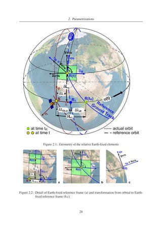
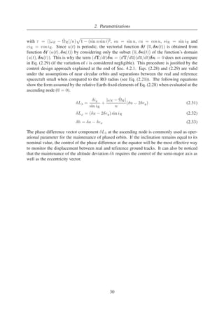
56. 3. Reference Orbit and Free Motion Analysis
Table 3.1.: Orbit specification in terms of nominal mean orbital elements
Orbit specification Related orbital elements
Space fluctuations of altitude exR(aR), eyR(aR)
Time fluctuations of altitude exR(aR, iR), eyR(aR, iR)
Local time aR(iR)
Phasing aR(iR)
Coverage iR
forces because usually the RO has to be completely periodic. Thus the reference orbit model
should at least consider the non-spherical terms of the Earth gravitational potential so that the
RO is an ideal orbit whose mean orbital elements are periodical functions with invariant max-imum
and minimum amplitudes. The nominal value of the orbital elements, which meet the
operational requirements, are obtained [3] by solving the orbital equations of motion including
only secular perturbations (in the case of sun synchronicity, phasing and altitude) and long pe-riod
perturbations (for the altitude) which are related to the geopotential. The result is a defined
relationship, dependent on the requirements, between different orbital elements as shown in Ta-ble
3.1. The level of accuracy of the nominal orbital elements’ numerical value is related to the
gravitational field model and the number of terms used. Only the zonal harmonics of even value
are considered for the secular variations and odd value for long-period variations. The elements
a, ex, ey determine the size, shape and orientation of the orbit within its plane whereas i and
characterize the orientation of the orbital plane. The value of the argument of latitude u does
not require any absolute specification as it represents the time variable. Several specifications
can be grouped for the design of a RO.
3.1.1. Altitude Requirements
The altitude variation constraints can be required in terms of space by minimizing the fluc-tuations
in relation to latitude on a given orbit segment or in terms of time by restricting the
fluctuations in time over a given point of the Earth surface and can be established through a
proper choice of a, ex and ey (e and ω).
Minimization of Spatial Fluctuations
The variation of altitude as a function of u taking into account the variations of a, ex and ey
must be examined to carry out the spatial minimization. Considering the expansion to the first
order in e of the altitude h = h(u,e) and assuming a near circular orbit, there will be a maximum
deviation hMAXe=0 relative to the mean hm at the equator and the extreme latitudes [3]
h(u) = hm − eam cos(u − ω) − (hMAX,e≈0) cos 2u (3.1)
hm = a
1 −
3
2
J2
RE
a
2
1 −
3
2
#
− RE
sin2 i
1 −
f
2
sin2 i
(3.2)
32

57. 3. Reference Orbit and Free Motion Analysis
hMAX,e≈0 = RE
f
2 −
J2
6
RE
a
sin2 i (3.3)
where f = 1 − ap/ae is the flattening parameter of the Earth ellipsoid [8] if ae and ap are
respectively its semi-major and semi-minor axes.
The minimization of altitude variations in the orbital quadrants q = 1, 2, 3, 4 corresponding
to u = [0, π/2], [π/2, π], [π, (3/2)π], [(3/2)π, 2π] leads to
ω =
3
4
π − (q − 1)
π
2
, e ≈ 1.57
hMAX,e≈0
a
(3.4)
hMAX,q =
1.57
√2 − 1
hMAX,e≈0 (3.5)
Minimization of Time Fluctuations
For the minimization of the altitude fluctuations in time, the variations of the mean orbital
elements e and ω have to be cancelled out [3]
de
dt
= f(a, e, ω, i) = 0 (3.6)
dω
dt
= g(a, e, ω, i) = 0 (3.7)
If the low frequency portion of the spectrum of perturbations of the geopotential is considered
(periods much longer than the orbital period) then the long-period variations affecting e and ω
are due to the odd number zonal terms of the geopotential whereas the secular variations affect
only ω and are related to the even number zonal terms. Adding these two effects, the solution of
Eq. (3.6) yields the frozen orbit conditions [23-28]. If only an expansion limited to J3 is used,
the approximate solution of Eq. (3.6) is
ω = ±
π
2
(3.8)
e ≈ −
J3
2J2
RE
a
sin i (3.9)
The majority of frozen orbits have ω = π/2. In both cases of ω = ±π/2 the altitude at a
given latitude is the same in the ascending and descending orbits disregarding the influence of
longitude via the tesseral terms of the potential.
3.1.2. Local Time Requirements
Sun synchronism is imposed through the relationship between a and i obtained by setting the
secular angular rotation of the line of nodes, due to the non-sphericity of the Earth, equal to the
known angular rotation of the meridian plane containing the mean Sun. The sun synchronism
condition [29,30] is thus represented by Eq. (3.10) where the averaged variation of
due to the
33

58. 3. Reference Orbit and Free Motion Analysis
first three zonal terms J2, J3 and J4 [21] is represented by Eq. (3.10).
˙
= !sy (3.10)
˙
= −
3
2
nJ2
RE
p
2
cos i −
3
2
nJ2
2
RE
p
4
cos i
9
4
+
3
2
p
1 − e2 − sin2 i
5
2
+
9
4
p
1 − e2
+
+
e2
4
1 +
5
4
+
sin2 i
e2
8
(7 − 15 sin2 i) cos 2!
−
3
8
nJ3
RE
p
3
(15 sin2 i − 4)e cot i sin !+
+
15
16
nJ4
RE
p
4
cos i
(4 − 7 sin2 i)
1 +
3
2
e2
− (3 − 7 sin2 i)e2 cos 2!
(3.11)
where ωsy = 1.99099299 × 10−7 rad s−1 is the mean apparent revolution speed of the Sun
around the Earth, RE = 6378140mis the equatorial p
radius of the terrestrial spheroid, p = a(1− e2) is the parameter of the orbit and n =
μ/a3 is the mean motion (with μ = 3.9860064 ×
1014 m3 s−2).
Eq. (3.10) imposes the constraints that the nominal drift of the line of nodes is frozen in
relation to the Earth-Sun direction and thus provides one of the two orbital element (a, i) as
function of the other. The semi-major axis of a sun-synchronous orbit has its upper boundary at
12.35 · 106 m for an inclination which tends to 180 deg. The inclination of a sun synchronous
orbit is always more than 90 deg
3.1.3. Phasing Requirements
A repeat-ground-track orbit [31-38] is obtained when there is a commensurability between the
satellite’s nodal frequency and the Earth’s rotation rate i.e. the time required by the satellite to
complete an integer number of orbits is equal to the total time required by the Earth to complete
an integer number of rotations. If TR and nR = 2π/TR are respectively the nodal period and
the nodal frequency, the condition for the ground track to repeat every k orbits in d days can be
formulated as [31]
ωE − ˙
nR
=
d
k
(3.12)
where ωE = 7.292115×10−5 rad s−1 is the Earth rotation rate, ˙
is the secular rotations of the
line of nodes.
If the zonal coefficients J2 and J4 of the geopotential are considered, the repeat-ground-track
condition of Eq. (3.12) can be explicitly formulated as [31]
N
D
=
d
k
N =
ωE
nJ2
a
RE
2
+
3
2
cos i −
15
16
J4
J2
RE
a
2
cos i(4 − 7 sin2 i)+
+
3
8
J2
RE
a
2
cos i(11 − 20 sin2 i)
34

59. 3. Reference Orbit and Free Motion Analysis
D = 1 + 3 −
15
4
sin2 i −
15
16
J4
J2
RE
a
2
34
5 − 25 sin2 i +
77
4
+
sin4 i
+
3
16
J2
RE
a
2
(14 + 17 sin2 i − 35 sin4 i)
The phasing of the orbit then define a relationship between a and i. With a defined repeat-ground-
track pattern and the operational inclination given, the corresponding mean semi-major
axis a can be found by using any standard numerical method.
3.1.4. Coverage Requirements
The payload access to targets observation is a key requirement in the design of an orbit. The tar-get
can be one location, specified by a latitude or longitude, or a region of interest on the Earth’s
surface. To this end, the design of the orbit must satisfy performance metrics that are specified
by the end user as the total time of coverage over a region, the access to daytime and nighttime
coverage, or the time required to access a different region, among others. The requirement for
coverage [39-41] of a terrestrial zone extending to a given latitude ϕ will determine, among
other parameters, an acceptable range of values for the inclination i between ϕ and π − ϕ if the
lateral field of view of the payload is not taken into account.
3.2. Reference Orbit Generation
Fig. 3.2 shows the detailed view of the block of Fig. 1.2 representing the RO generation process.
The deviations of the real from the reference orbital elements are defined by means of the
operational parameters (Sec. 2.2) or equivalently by means of the relative Earth-fixed elements
(Sec. 2.3.2). Table 3.2 collects the relationship between the orbit specifications, the operational
parameters, the REFE and the deviation of the real from the nominal orbital elements expressed
by means of relative orbital elements. The dependence of h on δix ≡ δi (Eq. (2.17)) has
not be considered as it is negligible on the short time scale. In Sections 3.2.1 and 3.2.2 the
fundamental issues regarding the RO generation will be analysed in detail. As a case study
the PRISMA mission (Sec. 1.4) is used since the analyses carried on in this section are strictly
related to the design and implementation of the on-board orbit control system validated in-flight
with the AOK experiment (Chap. 7).
Figure 3.2.: Reference orbit generation process
35

60. 3. Reference Orbit and Free Motion Analysis
Table 3.2.: Control specifications
Orbit specification Op. Parameter Rel. EF Element Rel. Orbital Element
Space fluctuations of altitude h δh δa, δex, δey
Time fluctuations of altitude h δh δa, δex, δey
Local time LT δL(0) - δL'(0)α* δiy
Phasing LAN δL(0) δey, δiy, δu
Coverage - - δix
*α = |ωE − ˙
R|/(n sin iR)
3.2.1. Reference Orbit Propagation Model
As explained in Sec. 3.1, the RO is generated by an orbit propagator which includes in the forces
model only the Earth gravitational field. The actual orbit of a spacecraft deviates from the RO
under the action of non-conservative perturbing forces. The goal of this section is to quantify the
contribution of the accuracy of the Earth’s gravitational field model used for the RO generation
to the deviation of the actual from the reference values of the operational parameters controlled.
To this end numerical simulations have been performed. In each simulation a propagated orbit
representing the actual trajectory of the MANGO spacecraft in free motion, has been compared
with a RO generated using a gravitational field model each time including a higher order and
degree number of harmonics (20x20, 30x30, 40x40, 50x50, 60x60 and 70x70). Tables 3.3 and
3.4 collect respectively the spacecraft physical properties and the force models used for the
propagation of the simulated actual and reference trajectories. The initial state used for the
orbit propagation is shown in Table 3.5 and the run time is one month (duration of the AOK
experiment). The POD ephemerides of the spacecraft TANGO, the PRISMA formation’s target
satellite which flies in free motion, have been exploited to calibrate the atmospheric density
model used for the simulations in order to have a high degree of realism. Fig. 3.3 shows the
difference between TANGO’s orbit as estimated by the POD process with an accuracy at the
sub-decimetre level and an orbit propagated with the calibrated model of Table 5.1. Figures 3.4-
3.8 show the comparison between the actual and the RO propagated with different models. In
Fig. 3.4 the comparison is done by means of relative orbital elements, whereas in Figures 3.6-
3.8 the evolution in time of the REFE is shown. It can be noted that in the RO generation
process, the use of a gravitational field model including an order and degree of harmonics lower
than 40x40 causes a propagation error. It can be stated therefore that a gravitational field model
Table 3.3.: PRISMA spacecraft physical properties
Spacecraft Physical Property MANGO TANGO
Mass [kg] 155.12 38.45
Drag area [m2] 0.5625 0.2183
Drag coefficient [-] 2.5 2.5
SRP effective area [-] 0.5625 0.2183
SRP [4] coefficient [-] 5.5 3.13
36

61. 3. Reference Orbit and Free Motion Analysis
Table 3.4.: Propagation parameters
Orbit Propagation Model
Earth gravitational field GRACE GGM01S 70x70
Atmospheric density Harris-Priester
Sun and Moon ephemerides Analytical formulas [4]
Solid Earth, polar and ocean tides IERS
Relativity effects First order effects
Numerical integration method Dormand-Prince, fixed step 1 s
RO Propagation Model
Earth gravitational field GRACE GGM01S nxn
Table 3.5.: Initial state - POD state on 20-06-2011 at 06:00:00 UTC
ECI state rR[m] rT[m] rN[m] vR[m/s] vT[m/s] vN[m/s]
-3967394.8566 -289822.105 5883191.2151 -6126.365 1487.7675 -4071.5062
Mean orb. el. a[m] ex[−] ey[−] i[deg]
[deg] u[deg]
7130522.2961 -0.004058 0.002774 98.28 351.74 123.38
including at least an harmonics order and degree of 40 should be used to avoid the inclusion of
orbit’s model errors in the generation of the RO. If the RO is generated on-board, the quality
of the gravitational field which can be used may be limited by the available computational
resources (see Chapter 7) and the errors introduced by the RO propagation model has to be
evaluated in relation to the control accuracy requirements.
Figure 3.3.: Difference between TANGO’s actual (POD) and propagated orbital elements
37

62. 3. Reference Orbit and Free Motion Analysis
Figure 3.4.: MANGO’s ROE (Actual-RO)
Figure 3.5.: MANGO’s REFE at the ascending node (Actual-RO)
38

63. 3. Reference Orbit and Free Motion Analysis
Figure 3.6.: MANGO’s δL at the ascending node (Actual-RO) - Details
Figure 3.7.: MANGO’s δL' at the ascending node (Actual-RO) - Details
39

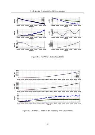
64. 3. Reference Orbit and Free Motion Analysis
Figure 3.8.: MANGO’s δh at the ascending node (Actual-RO) - Details
3.2.2. Accuracy Requirements of the Reference Orbit’s Initial State
This section is dedicated to the evaluation of the propagation error introduced by a bias in the
initial state used for the RO generation. The results of this analysis are relevant for the case
in which the RO is generated on-board using an actual state of the spacecraft (see Chapter 7).
The most accurate satellite state vectors available are those contained in the POD ephemerides
which, for the PRISMA spacecraft, are accurate at the sub-decimetre level. An alternative
source of absolute orbit information is the navigation filter integrated in the spacecraft on-board
computer. The values collected in Table 3.6 are representative of the spacecraft state estimation
errors on-board theMANGO spacecraft. Numerical simulations have been run to understand the
impact of the errors of the initial state on the propagation of the RO. Figures 3.9 and 3.10 show
the difference between the actual orbit and a RO propagated using initial states with different
accuracies. The different initial states used for the propagation of the RO are obtained from that
of Table 3.5 by adding the navigation error of Table 3.6 multiplied by 1, 2 and 3. All the orbits,
the actual and the reference, have been propagated using a 70x70 gravitational field model in
order to exclude oscillations due to different gravitational field harmonics modelling. From the
results shown in Figures 3.9 and 3.10 it can be stated that if the RO is generated on-board using
an actual state of the spacecraft, it is recommendable to use an uploaded POD state vector.
Table 3.6.: On-board navigation error
RTN_ECI state x[m] y[m] z[m] vx[m/s] vy[m/s] vz[m/s]
-3.0 -2.5 -1.0 -0.005 0.006 -0.002
40

65. 3. Reference Orbit and Free Motion Analysis
Figure 3.9.: MANGO’s ROE (POD-RO)
Figure 3.10.: MANGO’s REFE (POD-RO)
41

66. 3. Reference Orbit and Free Motion Analysis
3.3. Free Motion Analysis
A study of the orbital variations induced by the natural forces only [12-21], a free motion
analysis, shows that the real orbital elements will tend to diverge from their nominal values.
This leads to a violation of the flight control requirements defined by means of the operational
parameters (Table 3.2). Fig. 3.11 shows the detailed view of the subsystem of Fig. 1.2 repre-senting
the dynamics of the system when the control input v is zero, i.e. when the system
is in open-loop. From an analysis of the system in open-loop the evolution in time of mission
characteristics may be predicted and an orbit control strategy defined. The main natural forces
perturbing the ideal Keplerian spacecraft orbit are the non-spherical Earth gravitation field, the
Luni-solar gravitation, the atmospheric drag and the solar radiation pressure. The Earth and
Luni-solar gravitation are derived from a potential and may be treated analytically by means of
the Lagrange equations [8] whereas the other perturbations have to be treated with the Gauss
equations [5,2]. The evolution in time of each orbital element κi can be modelled [3] as
κi(t) = κ0 +
Xm
1
Aj sin
2π
t
Tj
+ φj
+
Xn
1
Bi(t − t0)i (3.13)
The first term of Eq. (3.13) represents the mean element associated with κi. The second term
is the periodic evolution of the orbital element with its period Tj , amplitude Aj and phase φj .
The third term represents the secular evolution of κi, which is an expansion in powers of the
time difference. It expresses the long-term trend of the orbital element at the time at which
the periodic effect becomes negligible in relation to the secular effect. The perturbations are
Figure 3.11.: Free motion
42

67. 3. Reference Orbit and Free Motion Analysis
classified in Table 3.7 according to the value of their period T. The natural evolution of the orbit
causes the operational parameters or the REFE to diverge from their nominal value (Table 3.2).
The free motion analyses carried on in the next sections, are based on the POD data of
PRISMA (Sec. 1.4) and TerraSAR-X/TanDEM-X (Sec. 1.5) which are representative of mis-sions
flying in LEO at respectively 700 and 500 km altitude. Main goal of these analyses is the
study of the orbital perturbation forces environment which is fundamental for the design of an
on-board orbit control system.
Table 3.7.: Influence of orbit perturbation forces on the orbital elements
Perturbation Short period Mean period Long period Secular
Tj ≤ Torb Torb Tj ≤ TE TE Tj
Geo-potential a, ex, ey, i,
a, ex, ey, i,
ex, ey ex, ey
Atmospheric drag a, ex, ey a a, ex, ey
Luni-solar i,
i,
Solar radiation ex, ey, i ex, ey, i
Torb = orbital period, TE = Earth rotation period
3.3.1. Free Motion of the MANGO Satellite
The first step of this analysis was the calibration (Sec. 3.2.1) of the propagator’s parameters
in order to obtain a computed orbit as near as possible to the real one over a long simula-tion
period. The POD ephemerides of the spacecraft TANGO of the PRISMA mission, the
formation’s target satellite which flies in free motion, have been exploited to calibrate the at-mospheric
density model used for the orbit propagations. Fig. 3.12 shows the evolution of the
relative orbital elements between the POD ephemerides and the RO (generated with the param-eters
of Tables 3.4-3.6) and between the propagated orbit and the RO. As one can see the orbit’s
propagation obtained over one month is very representative of the reality considering that the
PRISMA POD ephemerides [83-85] have an accuracy at the sub-decimetre level. Figures 3.13-
3.15 highlight the contributions of each orbital perturbation force to the deviation of the real
from the RO for the satellite MANGO flying in a near sun synchronous orbit at an altitude of
about 700 km. The perturbation forces (Table 3.4) are the atmospheric drag, the solar radiation
pressure and the luni-solar third body gravitational field. As shown in Figures 3.13 and 3.14 the
atmospheric drag and the solar radiation pressure affect the in-plane (δa, δex, δey, δu) relative
motion of the real from the RO and give a negligible contribution to the out-of-plane motion
(δix, δiy). On the other hand the contribution of the third body perturbation is relevant in the
out-of-plane relative motion and negligible in the in-plane. Considering the REFE computed
at the orbit’s ascending node (Equations (2.28)-(2.29) and Equations (2.31)-(2.33)) the atmo-spheric
drag has the major influence on the evolution in time of δL and δL' whereas the solar
radiation pressure give the main contribution to the evolution of δh.
43

68. 3. Reference Orbit and Free Motion Analysis
Figure 3.12.: TANGO’s ROE (POD-RO) - Propagator calibration
Figure 3.13.: MANGO’s in-plane ROE (Propagated-RO)
44

69. 3. Reference Orbit and Free Motion Analysis
Figure 3.14.: MANGO’s out-of-plane ROE (Propagated-RO)
Figure 3.15.: MANGO’s REFE at the ascending node (Propagated-RO)
3.3.2. Free Motion of the TerraSAR-X Satellite
The calibration of the propagator’s parameters for the case of the TerraSAR-X satellite is
shown in Fig. 3.16 which shows the evolution of the relative orbital elements between the POD
45

70. 3. Reference Orbit and Free Motion Analysis
Table 3.8.: Physical properties of the TerraSAR-X spacecraft
TSX Mass [kg] Drag and SRP area [m2] Drag coefficient [-] SRP coefficient [-]
1341.17 3.2 3.0 3.0
Table 3.9.: Propagation initial state
RTN_ECI state rR[m] rT[m] rN[m] vR[m/s] vT[m/s] vN[m/s]
4888898.0844 289059.4988 -4852522.5771 -5165.0722 -1691.6329 -5308.9558
Mean orb. el. a[m] ex[−] ey[−] i[deg]
[deg] u[deg]
6883553.0003 0.000026 0.001251 97.43 190.82 225.11
ephemerides and the RO and between the propagated orbit and the RO. In this case a free mo-tion
orbit arc of 7 days has been used as this is the maneuver cycle of TSX. The modelled forces
used for the propagation are the same of Table 3.4 whereas TSX’s physical propierties and the
propagation initial state are collected respectively in Tables 3.8 and 3.9. The initial state is the
POD state of TSX on 03-07-2011 at 06:00:00 UTC and the solar radiation pressure reference
area is the same as the drag area. Figures 3.17-3.19 highlight the contributions of each orbital
perturbation force to the evolution in time of the ROE and REFE. The same considerations of
the previous section are valid here. Despite the fact that the mass of TSX (Table 3.9) is about
ten times larger than the mass of MANGO (Table 3.4) the orbital decay rate of TSX is much
larger. This is due to the fact that as TSX flies at an altitude 200 km lower than MANGO the
atmospheric drag is stronger, and of course also to the larger drag area.
Figure 3.16.: TSX’s ROE (POD-RO) - Propagator calibration
46

71. 3. Reference Orbit and Free Motion Analysis
Figure 3.17.: TSX’s in-plane ROE (Propagated-RO)
Figure 3.18.: TSX’s out-of-plane ROE (Propagated-RO)
47

72. 3. Reference Orbit and Free Motion Analysis
Figure 3.19.: TSX’s REFE at the ascending node (Propagated-RO)
48

73. 4. Control Methods
This chapter deals with the regulator block of Fig. 1.2. As shown in Fig. 3.1, the regulator
receives as input the difference between the actual and nominal parameters to be controlled
and issues an orbital maneuver computed with a specific algorithm. Three types of control
algorithms are presented. The first is the one used in the AOK experiment (Chapter 7) on
the PRISMA mission. The AOK controller adopts a guidance law for the orbital longitude of
the ascending node and implements an analytical feedback control algorithm using along- and
anti-along-track velocity increments. The second and third controllers are the linear and the
quadratic optimal regulators from modern control theory. In the case of the analytical meth-ods
the mission dependent orbit’s requirements are translated into thresholds applied on some
operational parameters (Sec. 2.2) which specify the main features of the orbit’s ground track
geometry. The analytical model which describes the evolution of each operational parameter
in relation to the orbital elements allows then the definition of a control cycle. In the case of
the numerical feedback methods the problem is defined as a virtual formation control design
by means of the relative Earth-fixed elements (Sec. 2.3) and solved with the techniques of the
modern control theory. The analytical and numerical feedback control methods will be com-pared
by means of numerical simulations in Chapter 5 where some conclusions will be drawn
about the advantages and drawbacks in using and operating each type of orbit controller.
Figure 4.1.: Orbit regulator
4.1. Analytical Control of Phase Difference
Remote sensing satellites in LEO are often required to carry out repeat Earth coverage in order
to ensure identical geometric conditions of observation. If the orbit’s inclination can be assumed
to remain equal to its nominal value, controlling the phase difference at the equator will suffice
to keep the phasing of the orbit. This section is dedicated to an analytical method for the
49

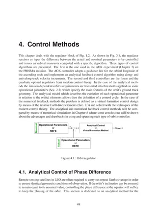
74. 4. Control Methods
control of the phase difference. Among the control methods presented in this chapter, only this
algorithm was validated in-flight with the AOK experiment on the PRISMA mission because it
had a most advanced implementation status at the moment of its selection.
4.1.1. Control Concept
Specific mission requirements are expressed by means of operational parameters [3] functions
of the orbital elements, which define the maximum allowed deviation of the actual from the
nominal trajectory of the spacecraft. Typical operational parameters (Sec. 2.2) are the altitude
deviation and phase difference at a certain latitude, local time deviation and in-orbit phasing
which specify the nominal position of the sub-satellite point in relation to a reference ground
track on the Earth’s surface [44]. The orbital elements of a spacecraft deviate from their nominal
values under the action of perturbing forces. Once the mission requirements have been trans-lated
into orbit control margins, it is necessary to compute the corrections to be applied to the
orbital elements to keep the value of the operational parameters within their control windows.
The following equations in the mean elements are the Gauss variational equations of motion
adapted for near-circular, non-equatorial orbits [3] and provide the relationships between the
velocity increments in the RTN orbital frame and the increments in the orbital elements.

a
ex
ey
i
u



=
1
v

0 2a 0
sin u 2 cos u 0
−cos u 2 sin u 0



0 0 cos u
0 0 sin u/ sin i
−2 0 −sin u/ tan i


vR
vT
vN

 (4.1)
where v is the spacecraft’s velocity magnitude. The implementation of an orbit control strat-egy
implies the specification not only of the magnitude of the corrective maneuvers but also
the geometric and time characteristics which maximize their efficiency. The choice of the less
expensive maneuvers’ in-orbit location depends on the operational parameter that has to be
controlled. An out-of-plane maneuver vN to change the orbit’s inclination, for example, ac-cording
to the Gauss equations (Eq. (4.1)) is most effective if placed at the node (u = 0) while
at the orbit’s highest latitude (u = π/2) if
has to be changed. On the other hand, while the
semi-major axis can be changed with an along-track maneuver vT with the same effectiveness
anywhere along the orbit, the vT most effective [74] to control δL (Eqs. (2.31)-(2.33)) has to
be computed at the equator (ascending or descending node) for reasons of symmetry.
4.1.2. Basic Orbit Keeping Strategy
Referring to Eq. (2.10) if da/dt and di/dt are taken as constants, LAN is found to have a near
parabolic variation as its second derivative is constant. A positive LAN means that the ground
track of the satellite at the equator lies eastwards with respect to the reference track. This means
that if it is assumed that the semi-major axis has a linear decay under the influence of the atmo-spheric
drag, the real orbit LAN will move parabolically eastwards of the reference LAN. Based
50

75. 4. Control Methods
Figure 4.2.: Maneuver with estimated da/dt
on this consideration a simple control cycle can be imposed [3]. When the deviation between
the real and nominal LAN exceeds a pre-defined upper bound LMAX a correcting impulse in
the along-track direction of the satellite’s orbit is applied as much as twice as would be neces-sary
in order to return to the initial semi-major axis’ value. As a result, just after the impulse
the satellite’s LAN begins to move westward, reaches the lower bound of the allowable band
and drifts back to the upper limit where the next correction maneuver is made. The theoretical
maneuver cycle T and the semi-major axis increments ac to be applied (Fig. 4.2) can thus be
obtained from Eq. (2.10) assuming also that di/dt is negligible compared to da/dt [3].
ac =
1
2
s
K

79. da
dt

83. Lc (4.2)
51

84. 4. Control Methods
T =
s
K

88. da
dt

92. −1
Lc (4.3)
K =
16
3π
a
RE
TE (4.4)
with Lc = LMAX in steady state phase (no RO acquisition). From the Gauss equations
adapted for circular orbits, the velocity increment to be applied is
v =
ac
2a
v (4.5)
where v is the satellite velocity. By considering Eqs. (4.2) and (4.5) it is straightforward to
conclude that a correct and fine estimation of the maneuver is strictly connected to a correct
estimation of da/dt which is mainly determined by the atmospheric drag. Fig. 4.2 shows the
possible evolutions of the LAN deviation after a maneuver based on different estimated values
of da/dt. It is evident that if da/dt has been underestimated the v applied results in a ac
that is smaller than necessary to impose an optimal maneuver cycle period. On the other hand
if da/dt has been overestimated the v applied results in a a that is too large and the negative
LAN deviation exceeds the lower dead-band −LMAX resulting in requiring an anti-along-track
maneuver to keep the LAN value within the control window. The better the estimation
of da/dt, the closer the realized maneuver cycle will be to the ideal one thus minimizing the
number of required maneuvers (Fig. 4.2).
4.1.3. Reference Orbit Acquisition
A fundamental requirement of an autonomous orbit control is to bring back the LAN devia-tion
within the control window limits ±LMAX starting from an error which has a magnitude
greater than the allowed threshold. This type of maneuver can be requested to be optimal in the
sense that it minimizes the amount of fuel required and can be required to be performed within
certain time constraints. If no time requirements are enforced, an optimal maneuver will impose
aac that will let the LAN to drift in free motion, with respect to the reference, along a parabola
whose vertex lays on the minimum threshold of the control window. Referring to Fig. 4.3 in
general the maneuver’s ac for a RO acquisition is given by Eq. (4.2) where the proper Lc
can be computed given an initial phase difference Lini and a time constraint. Imposing an
initial semi-major axis displacement ac with an along-track maneuver, the evolution of the
LAN error can be represented in the plane t − L by a parabola of equation
L =
8Lc
T2 t2 −
8Lc
T
t + Lini (4.6)
with T given by Eq. (4.3). The time required for the return of the LAN error within the control
window limits is then the intersection of parabola of Eq. (4.6) with line of equation L =
52

93. 4. Control Methods
Figure 4.3.: Smooth and timed RO acquisition from positive LAN deviation values
LMAX
tc =
T
2

1 −
1
2
s
4 +
2(LMAX − Lini)
Lc

 (4.7)
Imposing that tc ∈ ℜ and tc ≥ 0, the following conditions on Lc and Lini are obtained
Lc ≥
Lini − LMAX
2
and Lini ≥ LMAX (4.8)
Smooth Maneuver
If the RO acquisition has to be performed with the only requirement ofminimizing themaneuver
size with no time constraints, the vertex ordinate of the parabola of Eq. (4.6) will be imposed to
be equal to −LMAX i.e. placed on the lower threshold of the control window. In the ideal case
this kind of maneuver, indicated as smooth in Fig. 4.3, does not require any further correction
to the initial v. The resulting Lc is then
Lc =
Lini + LMAX
2
(4.9)
53

94. 4. Control Methods
and the acquisition time is
tsmooth =
T
2
1 −
r
LMAX
Lc
!
=
1
2
s
K

98. da
dt

102. −1
Lc
1 −
r
2LMAX
LMAX + Lini
!
(4.10)
with K given by Eq. (4.2). The RO acquisition maneuver is computed with Eqs. (4.2) and (4.5)
using Lc given by Eq. (4.9).
Timed Maneuver from positive deviation
If a time constraint tc ≤ τ is imposed and tsmooth τ , where τ is a fixed time interval, a timed
maneuver is required as indicated in Fig. 4.3. If the initial phase difference deviation Lini has
a positive value, Eq. (4.7) can be solved for Lc imposing tc = τ and T given by Eq. (4.3) and
yields
Lc =
1
K

106. da
dt

110. K

114. da
dt

118. −1 (Lini − LMAX)
8τ
+ τ
#2
(4.11)
where K is given by Eq. (4.2). The RO acquisition maneuver is computed with Eqs. (4.2)
and (4.5) using Lc given by Eq. (4.11). This kind of maneuver requires an anti-along-track
counter-maneuver when the negative LAN deviation reaches the lower deadband −LMAX.
Timed Maneuver from negative deviation
If the initial phase difference deviation has a negative value, the problem can be solved by
considering Fig. 4.4. The value of −ac has to be found such that starting from an initial value
−Lini, L will evolve in time on the timed maneuver parabola of Eq. (4.12) thus fulfilling
the RO acquisition time constraint.
L1 =
8Lc
T2 t2
1 − Lc =
8
K
da
dt
t2
1 − Lc (4.12)
The parabola of Eq. (4.12) is written in coordinates t1,L1 obtained from t,L with the co-ordinates
transformation t1 = t + t , L1 = L. Imposing that points of coordinates
(t,−Lini)1 and (t + τ,−LMAX)1 belong to the parabola of Eq. (4.12) it results
t =
τ
2
K

122. da
dt

126. −1 (Lini − LMAX)
8τ 2 − 1
#
(4.13)
Lc =
(Lini − LMAX)
2
K

130. da
dt

134. −1 (Lini − LMAX)
16τ 2 − 1
#
+
2τ 2
K

138. da
dt

142. +Lini (4.14)
where K is given by Eq. (4.2). The anti-along-track RO acquisition maneuver is computed with
Eqs. (4.2) and (4.5) using Lc given by Eq. (4.14).
54

143. 4. Control Methods
Figure 4.4.: Timed RO acquisition from negative LAN deviation values
4.1.4. On-board Atmospheric Drag Estimation
As atmospheric density has a remarkable variability over time mainly due to fluctuations in the
solar flux (see Appendix D) an atmospheric model cannot provide the necessary accuracy for
strict LAN control requirements. On the other hand, as in case of theMANGO satellite, it is not
always possible to have on-board accelerometers accurate enough ( 10−5 m/s2) to extrapolate
the drag acceleration from their measurements. Nevertheless da/dt can be estimated on-board
using the actual orbit’s semi-major axis estimated by the navigation filter with an accuracy
of 4 m 1σ (see Sec. 7.1.8) and the RO. The value of da/dt is then found with the following
procedure explained with the help of Fig. 4.5. The actual and reference semi-major axis data
are first filtered by taking their values at the ascending node and smoothed if required. The
difference aAN between the actual and reference semi-major axis values is computed. The
value of da/dt is finally found as the slope of the line representing the linear fit over the time
of a sample of aAN data. A smoothing process of the on-board estimated values of aAN is
required in the computation of da/dt in presence of noise due to short period harmonics not
included in the gravitational field model used for the RO propagation or errors in the on-board
estimation of aAN. Fig. 4.5 shows the comparison of the aAN curves obtained with a RO
55

144. 4. Control Methods
Figure 4.5.: On-board estimation process of da/dt
generated with a 70x70 gravitational field model and one generated with a 5x5 model. The real
orbit is generated by numerical orbit propagation including the aspherical Earth gravitational
field (GGM01S model) through an expansion in spherical harmonics up to degree and order 70,
tides and relativity gravitational field perturbations, the Sun and Moon third body forces, the
atmospheric drag (atmospheric density model Harris-Priester) and solar radiation pressure. It
can be noticed in Fig. 4.5 that in the case of the 5x5 orbit model a short period (for example 10
points) linear fitting without data smoothing is totally unreliable for estimating the atmospheric
drag. A long period (50 points) linear fitting would allow an accurate estimation of da/dt, but
requires a minimum maneuver cycle period of 50 orbits (i.e. more than 3 days) which could be
too long as in the case of the AOK controller (Chapter 7). Nevertheless an efficient estimation
of da/dt is still possible using samples of 10 aAN values with a proper smoothing process.
The smoothing filter takes as input the points marked by circles in Fig. 4.5 and flattens them on
a line λ keeping unaltered the ratios of their distances from it. Line λ is defined by point (x1, y)
and angular coefficient m where x1 is the x-coordinate of the first point, y is the mean of the
y-coordinates of all the points of the sample andm is the estimated da/dt. The smoothed points
yksth are computed with the following equations
yksth = mxk + q ±
d√1 + m2
f
(4.15)
d = |yk − (mxk + q) √ | 1 + m2
q = y − mx1 (4.16)
where in the second term of Eq. (4.15) the + sign has to be used if yk ≥ mxk + q, the − sign
if yk mxk + q and f ≥ 1 is a flattening coefficient uploaded by TC. An initial value of
da/dt, estimated on-ground and uploaded to the spacecraft, is used for the very first smoothing
56

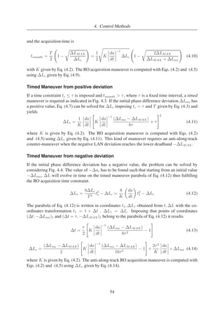
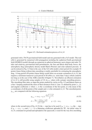
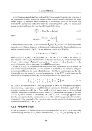
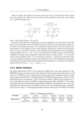
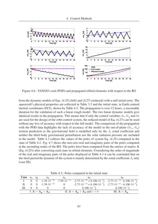
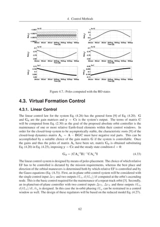
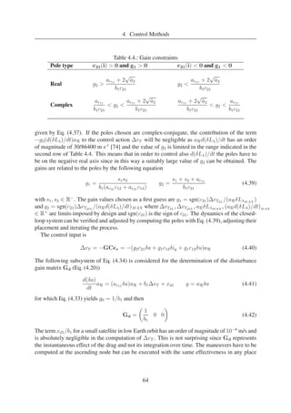
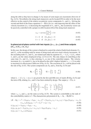
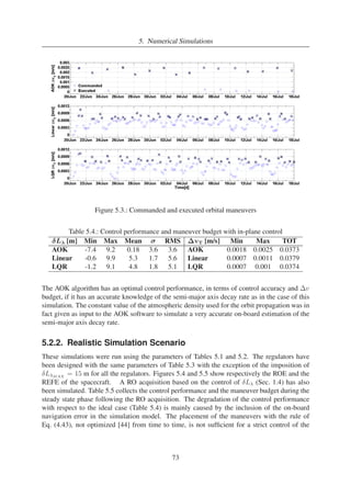
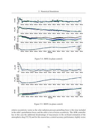
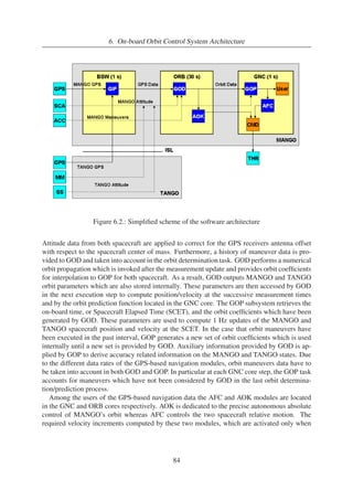
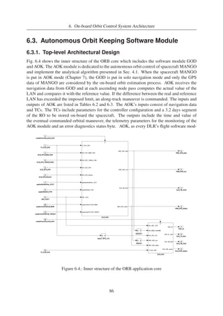
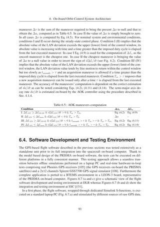
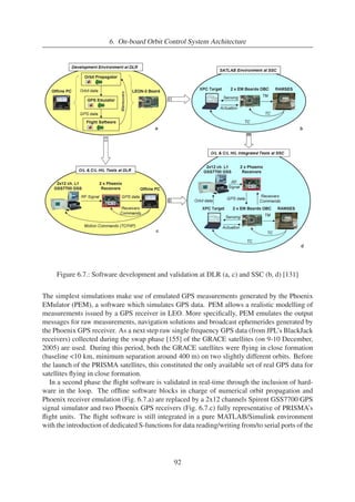
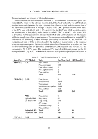
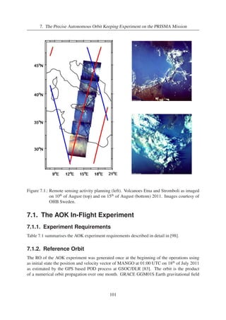
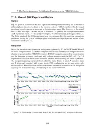
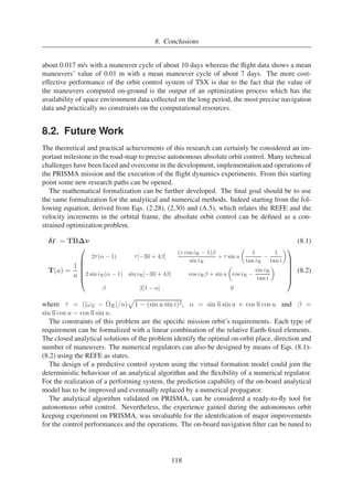
145. 4. Control Methods
process. The output points yksth of the smooth filter are marked by triangles in Fig. 4.5. If the
RO is generated with a 70x70 gravitational field model no data smoothing is required.
The AOK controller uses a GRACE GGM01S 20x20 gravitational field model for the on-board
RO generation (Sec. 7.1.2) and a sample buffer of 10 aAN’s which is renewed at each
ascending node passage with a first-in-last-out logic so thus the last 10 orbits data are always
stored in the buffer. The buffer is reset after each maneuver. In case no fitting is possible
because there isn’t a sufficient number of samples in the buffer, the da/dt is estimated using the
first of the Gauss equations (Eq. (4.1)) approximated for circular orbits [3]
da
dt
= −
ρ
B
√μa (4.17)
where ρ is the atmospheric density from the Harris-Priester model, B = m/(ACD) is the
ballistic coefficient of the satellite and μ = 3.9860064 × 1014 m3 s−2.
4.2. Virtual Formation Model
This section analyses the problem of the autonomous orbit control of a satellite in LEO using
the linear and the quadratic optimal regulators from the classical control theory [9, 10]. For
the implementation of the linear regulators the problem has been formulated as a specific case
of two spacecraft in formation in which one, the reference, is virtual and affected only by the
Earth’s gravitational field. The control action is realized by means of in-plane and out-of-plane
velocity increments. The state-space representation approach is used here for the realization of
the autonomous orbit control with techniques from modern control theory. In general, the linear
model used has state-space representation form
˙ ǫ = Aǫ + Bv + xd (4.18)
y = Cǫ (4.19)
v = −Gy −Gdxd (4.20)
where ǫ is the state vector, A and B are respectively the dynamic model and control input
matrix, xd is the modelled state perturbation, v is the impulsive velocity increment vector,
and G and Gd are, respectively, the output and disturbance gain matrices. The output vector y
is comprised of relative Earth-fixed elements introduced by Eq. (2.28).
4.2.1. Linear Dynamic Model
The state-space model of the orbital motion of the real and reference spacecraft is given by
˙ κ = ˜A
g(κ) + ˜A
d(κ) (4.21)
˙ κR = ˜A
g(κR) (4.22)
where κ = (a, ex, ey, i,
, u) is the mean orbital elements vector.
57

146. 4. Control Methods
Vector functions ˜A
g and ˜A
d (Eqs. (A.1) and (A.3) in Appendix A) describe the behaviour of
the mean orbital elements κ under the influence of the J2 gravitational perturbation and atmo-spheric
drag [5,21]. The mean orbital elements κR of the reference spacecraft are affected only
by the Earth’s gravitational field as they define the nominal trajectory [3,32]. The linearization
around κR of the difference between Eqs. (4.21) and (4.22) yields
d(δκ)
dt
= ˜A
(κR)δκ + ˜A
d(κR) (4.23)
where
˜A
(κR) =
∂[˜A
g(κ) + ˜A
d(κ)]
∂κ

151. R
(4.24)
is the Jacobian evaluated at κR of the vectors sum ˜A
g(κ)+˜A
d(κ), and δκ is the relative orbital
elements vector. Making the proper modifications to matrix ˜A
(κR) for the normalization in aR
and the introduction of δiy (Eq. (2.19)), and adding the control term B(κ)v:
˙ ǫ = A(κR)ǫ + xd + B(κ)v (4.25)
where A(κR) = Ag(κR) + Ad(κR) (Eqs. (A.2) and (A.4)), ǫ = aRδκ is the relative or-bital
elements vector (Eq. (2.19)) normalized to the semi-major axis, xd results from the direct
(dyadic) vectors product (˜A
d(κR))(1, aR, aR, 1, 1, 1)T and v = (vR,vT ,vN)T is the
vector of impulsive velocity increments in the RTN orbital frame.
Matrix B(κ) (Eq. (A.5)) represents the Gauss variational equations of motion adapted for
near-circular non-equatorial orbits [3]. The elements of matrix B(κ) are computed with good
approximation [5] using the mean orbital elements. The Gauss equations provide the rela-tionships
between the impulsive velocity increments vs in the RTN orbital frame and the
increments of the orbital elements. Eq. (4.25) can be written in the general form
˙ ǫ
˙xd
=
A I
0 A0
ǫ
xd
+
B
0
v (4.26)
Eq. (4.26) is the representation of a tracking system [9] in which the atmospheric drag pertur-bation
vector xd is represented as an additional state variable, the disturbance input, which is
assumed to satisfy the model ˙xd = A0xd and I is the 6x6 identity matrix. If the feedback
controller is designed to compute the control inputs vj always in the same place of the orbit
(u = u), xd can be assumed as constant (Eq. (A.3)) i.e. A0 ≡ 0. This design approach stems
from the consideration that the implementation of an orbit control strategy implies the specifica-tion
not only of the magnitude of the corrective maneuvers but also the in-orbit location which
maximizes their efficiency (Sec. 4.1.1).
4.2.2. Reduced Model
In case no eccentricity or inclination are to be actively controlled, the model can be reduced by
considering only the states δa, δiy and δu. The elements aij = agij+adij are given by Eqs. (A.2)
58

152. 4. Control Methods
and (A.4). The use of this model allows the design of a linear controller for the relative Earth-fixed
elements δL and δL'. The passive control of δh can be achieved by a proper in-orbit
placement of the along-track maneuvers as explained in the next section.
Ar =
3
4
a
RE
2 nJ2
(1 − e2)2


a11 0 0
a51 0 0
a61 0 0

 ǫr = aR


δa
δiy
δu


(4.27)
Br =
1
n



 xdr = −
0 2 0
0 0 sin u
−2 0 −sin u/ tan i
A
m
CDρ




√μa
0
0
If the reduced model of Eq. (4.27) is used, Eqs. (2.28)-(2.30) can be written, considering only
the states δa, δiy and δu, as
δ̥(u, ǫr)aR = Tr(u)ǫr
d(δ̥)
dt
aR = Tr(u)Arǫr (4.28)
Tr(u) =


−
3
2
uτ
τ (1 − cu)ciR
cu
+ 1
cu
siR
τ
−
3
2
usiR (1 − cu)ciR siR
1 0 0


(4.29)
4.2.3. Characteristic Polynomial
The characteristic polynomial of matrix A of Eq. (4.25) has the form
|sI − A| = s2(s − a11)(s3 + bs2 + cs + d) (4.30)
b = −(a22 + a33) c = a22a33 − a26a62 − a36a63 − a23a32 (4.31)
d = a26(a62a33 − a63a32) + a36(a63a22 − a23a62) (4.32)
and the elements aij of matrix A are given by the summation of Eqs. (A.2) and (A.4).
Table 4.1.: Analytic expressions of the poles
Case s1 s2 s3 s4 s5 s6
I. 0 0 a11 v + z −
b
3 −
1
2
(v + z) −
b
3
+
√3
2
(v − z)j −
1
2
(v + z) −
b
3 −
√3
2
(v − z)j
II. 0 0 0 a11 −α
r
μ
a − β(5 cos2 i − 1)j −α
r
μ
a
+ β(5 cos2 i − 1)j
III. 0 0 0 0 −β(5 cos2 i − 1)
r
3e2 + 1
e2 − 1
j β(5 cos2 i − 1)
r
3e2 + 1
e2 − 1
j
I. A = Ag + Ad II. A = Ag + Ad and e = 0 III. A = Ag
59

153. 4. Control Methods
Table 4.1 collects the analytic expressions of the roots of Eq. (4.30), the poles of the system
[9], in the general case with non-zero (I) and zero (II) eccentricity and in the case in which
A ≡ Ag (III) (no drag), with
α =
A
m
CD β =
3
4
RE
a
2
nJ2
v =
s
3
r
2
+
r
q3
27
+
r2
4
z =
s
3
r
2 −
r
q3
27
+
r2
4
q =
3c − b2
9
r =
9bc − 27d − 2b3
54
and b, c and d given by Eqs. (4.31)-(4.32).
The poles in the origin have multiplicity 2 in case I, multiplicity 3 in case II and 4 in case III.
Thus, in every case the system is not stable in the sense that at least one initial state ǫ(0) exists
for which ǫ will diverge over time. It is worthwhile to point out that in case III, the poles are
representative of the solutions of the system dynamics unforced by external non-conservative
forces. In cases I and II the system is in fact rendered non-homogeneous by the atmospheric
drag perturbation force ( ˙ ǫ = Aǫ + ˜A
d). In case III where the Earth’s gravity is the only force
modelled, the unique initial condition for which the system is stable is ǫ(0) = 0. In case III
with an initial condition ǫ(0)6= 0, δa will remain constant, δu will diverge and all the other
states, the components of the eccentricity and inclination vectors, will be affected by long period
perturbations due to the Earth’s gravitational field zonal coefficient J2. The poles of the reduced
system of Eq. (4.27) are s1 = 0, s2 = 0 and s3 = a11.
4.2.4. Model Validation
The POD ephemerides [83,85] of the spacecraft TANGO [92], the target spacecraft of the
PRISMA formation, have been used for the validation of the linear dynamicmodels of Eqs. (4.25)
and (4.27). TANGO is in free motion not having any orbit control capability and has an orbit
almost identical toMANGO’s. The POD positions of TANGO provide a picture of the real orbit
perturbation forces environment. In Fig. 4.6 the lines noted as POD are the evolution over 3
days of the difference between TANGO’s orbital elements and a RO. The RO [73, 74] has been
generated using a gravitational field model (GRACE GGM01S, 70x70 degree-order) as the only
modelled force. The initial state of the RO is the first state of the POD ephemerides considered
and is given in Table 4.2. The propagated relative elements with respect to the RO are obtained
Table 4.2.: Propagation parameters
ECI state rR[m] rT[m] rN[m] vR[m/s] vT[m/s] vN[m/s]
-3967394.8566 -289822.105 5883191.2151 -6126.365 1487.7675 -4071.5062
Mean orb. el. a[m] ex[−] ey[−] i[deg]
[deg] u[deg]
7130522.2961 -0.004058 0.002774 98.28 351.74 123.38
60

154. 4. Control Methods
Figure 4.6.: TANGO’s real (POD) and propagated orbital elements with respect to the RO
from the dynamic models of Eqs. (4.25) (full) and (4.27) (reduced) with a null initial error. The
spacecraft’s physical properties are collected in Table 3.3 and the initial state, in Earth centred
inertial coordinates (ECI), shown by Table 4.2. The propagation is over 12 hours, a reasonable
duration for the validation of such a linear rough model. The two linear dynamic models give
identical results in the propagation. This means that if only the control variables δa, δiy and δu
are used for the design of the orbit control system, the reduced model of Eq. (4.27) can be used
without any loss of accuracy with respect to the full model. The comparison of the propagation
with the POD data highlights the lack of accuracy of the model in the out-of-plane (δix, δiy)
motion prediction as the gravitational field is modelled only by the J2 zonal coefficient and
neither the third body gravitational perturbation nor the solar radiation pressure are included
in the model. Table 4.3 collects the values of the poles of system Eq. (4.25) computed in the
state of Table 4.2. Fig. 4.7 shows the non-zero real and imaginary parts of the poles computed
at the ascending nodes of the RO. The poles have been computed from the entries of matrix A
(Eq. (4.25)) after converting each state in orbital elements. Considering the order of magnitude
of the real and imaginary parts of the poles displayed in Table 4.3 it can be concluded that on
the short period the dynamic of the system is mainly determined by the zonal coefficient J2 only
(case III).
Table 4.3.: Poles computed in the initial state
Case s1 s2 s3 s4 s5 s6
I. 0 0 -1.38·10−12 -7.95·10−14 -2.73·10−12 + 6.106·10−7j -2.73·10−12 - 6.106·10−7j
II. 0 0 -1.38·10−12 0 -2.73·10−12 + 6.106·10−7j -2.73·10−12 - 6.106·10−7j
III. 0 0 0 0 6.106·10−7j -6.106·10−7j
I. A = Ag + Ad II. A = Ag + Ad and e = 0 III. A = Ag
61

155. 4. Control Methods
Figure 4.7.: Poles computed with the RO states
4.3. Virtual Formation Control
4.3.1. Linear Control
The linear control law for the system Eq. (4.26) has the general form [9] of Eq. (4.20). G
and Gd are the gain matrices and y = Cǫ is the system’s output. The terms of matrix C
will be computed from Eq. (2.30) as the goal of the proposed absolute orbit controller is the
maintenance of one or more relative Earth-fixed elements within their control windows. In
order for the closed-loop system to be asymptotically stable, the characteristic roots [9] of the
closed-loop dynamics matrix Ac = A − BGC must have negative real parts. This can be
accomplished by a suitable choice of the gain matrix G if the system is controllable. Once
the gains and thus the poles of matrix Ac have been set, matrix Gd is obtained substituting
Eq. (4.20) in Eq. (4.25), imposing y = Cǫ and the steady state condition ˙ ǫ = 0:
c B)−1CA−1
c I (4.33)
Gd = (CA−1
The linear control systemis designed bymeans of poles placement. The choice of which relative
EF has to be controlled is dictated by the mission requirements, whereas the best place and
direction of the orbital maneuvers is determined both by which relative EF is controlled and by
the Gauss equations (Eq. (A.5)). First, an in-plane orbit control system will be considered with
the single control input vT and two outputs δL, d(δL)/dt computed at the orbit’s ascending
node. This is the basic control required for the maintenance of a repeat-track orbit [3]. Secondly,
an in-plane/out-of-plane controller with two control inputs vT , vN and three outputs δL,
d(δL)/dt, δiy is designed. In this case the in-orbit phasing δL' can be restrained in a control
window as well. The design of these regulators will be based on the reduced model Eq. (4.27).
62

156. 4. Control Methods
In-plane control with one input (vT) and two outputs (δL, d(δL)/dt)
In this case, the design of the feedback system is finalized to control δL and d(δL)/dt, com-puted
at the ascending node (Eqs. (2.31)-(2.33)), by means of along-track velocity increments.
This means that the orbit controller is designed to work only once per orbit at most. The system
components are
Ar =



 ǫr = aR
ar11 0 0
ar21 0 0
ar31 0 0


δa
δiy
δu

 Br =


b1
0
0


(4.34)
G =
g1 g2
Gd =
g0 0 0
xdr =


xd1
0
0


with ar11 , ar21 , ar31 , b1 = 2/n, xd1 given by Eq. (4.27) and g1, g2 ∈ R. The output y = Cǫr is
aR
δL
d(δL)
dt
!
= aR
0 c12 c13
c21 0 0


δa
δiy
δu

 (4.35)
where the terms c12 = 1/ sin iR, c13 = |ωE − ˙
R|/n and c21 = ar21/ sin iR + ar31 |ωE − ˙
R|/n
are obtained from Eqs. (4.28)-(4.29) imposing u = 0.
The control input is given by vT = −(g1δL + g2d(δL)/dt)aR. The objective here is
to find the gains g1 and g2 which place the poles of the closed-loop dynamic matrix Ac =
Ar − BrGC at the locations desired. The characteristic polynomial of Ac is
|sI − Ac| = s[s2 + (b1c21g2 − ar11)s + b1(ar21c12 + ar31c13)g1] = s[s2 + ˆa1s + ˆa2] (4.36)
ˆa1(g2) = b1c21g2 − ar11 ˆa2(g1) = b1(ar21c12 + ar31c13)g1 (4.37)
One of the three poles of Ac is placed in the origin regardless of the value of the gains. This is
due to the fact that the part of the system depending on δiy is not controllable by vT . Indeed
the controllability test matrix
Qctr =
B ArBr A2
rBr
=


b1 ar11b1 a2
r11b1
0 ar21b1 ar11ar21b1
0 ar31b1 ar11ar31b1

 (4.38)
has rank 2, smaller than the maximum rank 3. Nevertheless at the ascending node δL =
k1δiy +k2δe+k3δu ((Eqs. (2.31)-(2.33))) can be controlled by means of variations p
of δu which
compensate the variations of δiy and δe. The closed-loop poles s = (−a1 ˆ±
ˆa2
1 − 4ˆa2)/2 of
Eq. (4.36) are real (complex-conjugate) if |ˆa1| = 2√ˆa2 (|ˆa1| 2√ˆa2) and ˆa2 = b1c21g1
0. If ˆa1 0 the poles are placed on the left of the imaginary axis of the complex plane
and the closed-loop system is stable. If If ˆa1 0 the system is not stable. These stability
conditions impose constraints on the value of the gains as resumed by Table 4.4 where ˆa2 is
63

157. 4. Control Methods
Table 4.4.: Gain constraints
Pole type c21(i) 0 and g1 0 c21(i) 0 and g1 0
Real g2
ar11 + 2√ˆa2
b1c21
g2
ar11 + 2√ˆa2
b1c21
Complex
ar11
b1c21
g2
ar11 + 2√ˆa2
b1c21
ar11 + 2√ˆa2
b1c21
g2
ar11
b1c21
given by Eq. (4.37). If the poles chosen are complex-conjugate, the contribution of the term
−g2(d(δL)/dt)aR to the control action vT will be negligible as aRd(δL)/dt has an order
of magnitude of 30/86400 m s-1 [74] and the value of g2 is limited in the range indicated in the
second row of Table 4.4. This means that in order to control also d(δL)/dt the poles have to
be on the negative real axis since in this way a suitably large value of g2 can be obtained. The
gains are related to the poles by the following equation
g1 =
s1s2
b1(ar21c12 + ar31c13)
g2 =
s1 + s2 + ar11
b1c21
(4.39)
with s1, s2 ∈ R−. The gain values chosen as a first guess are g1 = sgn(c21)vTL/(aRδLMAX )
and g2 = sgn(c21)vTdL/(aRd(δL)/dt)MAX wherevTL,vTdL, aRδLMAX, (aRd(δL)/dt)MAX
∈ R+ are limits imposed by design and sgn(c21) is the sign of c21. The dynamics of the closed-loop
system can be verified and adjusted by computing the poles with Eq. (4.39), adjusting their
placement and iterating the process.
The control input is
vT = −GCǫr = −(g2c21δa + g1c12δiy + g1c13δu)aR (4.40)
The following subsystem of Eq. (4.34) is considered for the determination of the disturbance
gain matrix Gd (Eq. (4.20))
d(δa)
dt
aR = (ar11δa)aR + b1vT + xd1 y = aRδa (4.41)
for which Eq. (4.33) yields g0 = 1/b1 and then
Gd =
1
b1
0 0
(4.42)
The termxd1/b1 for a small satellite in low Earth orbit has an order ofmagnitude of 10−8 m/s and
is absolutely negligible in the computation of vT . This is not surprising since Gd represents
the instantaneous effect of the drag and not its integration over time. The maneuvers have to be
computed at the ascending node but can be executed with the same effectiveness in any place
64

158. 4. Control Methods
along the orbit as they have to change δu by means of semi-major axis increments (first row of
Eq. (A.5)). Nevertheless the along-track maneuvers can be located [92] in order to be the most
effective on the control of the relative eccentricity vector components δex and δey. Solving the
second and third of the Gauss equations ˙ ǫ = B(κ)v in u and imposing that the effect of the
velocity increment vT is decreasing the magnitude of δex and δey, the eccentricity vector can
be passively controlled with a proper in-orbit location [44] of the along-track maneuver:
uM = arctan
δey
δex
+ kπ (4.43)
k = 0 if (δexvT ) 0 (4.44)
k = 1 if (δexvT ) 0 (4.45)
In-plane/out-of-plane control with two inputs (vT, vN) and three outputs
(δL, d(δL)/dt, δiy)
In this case, the design of the system is finalized to control the relative Earth-fixed elements δL
and δL' at the ascending node by means of along-track and cross-track velocity increments. At
the ascending node δL and δL' are related each other by equation δL = k1δiy+k2δL' where
k1 and k2 are the values displayed in Eqs. (2.31)-(2.33). The only chance of controlling at the
same time δL and δL' is thus selecting δiy as one of the controlled outputs. The velocity
increment vN to control δiy has to be placed at the orbit’s highest latitude (u = π/2) in order
to maximize its effectiveness (fifth row of Eq. (A.5)). The execution of vT will be placed with
the rule of Eq. (4.43). The system components are Ar and ǫr from Eq. (4.34) and
Br =


b1 0
0 b2
0 0

 G =
g1 g2 0
0 0 gN
(4.46)
where b1 = 2/n, b2 = sin u/n are given by the first and fifth rows of matrix B (Eq. (A.5)) and
the term of Br relating vN and δu has been omitted by design. The output y = Cǫr is
aR


δL
d(δL)
dt
δiy


= aR


0 c12 c13
c21 0 0
0 1 0




δa
δiy
δu

 (4.47)
where c12, c13 and c21 are the same as in Eq. (4.35). The system is controllable as the rank of
the controllability matrix is 3. The characteristic polynomial of Ac = Ar − BrGC is
|sI − Ac| = s3 + (b1g2c21 + b2gN − ar11)s2 + [b1g1(ar21c12 + ar31c13) + b2gN(b1g2c21 − ar11)]s
+ar31c13b1b2g1gN = s3 + ˆa1s2 + ˆa2s + ˆa3 (4.48)
ˆa1(g2, gN) = b1g2c21 + b2gN − ar11 (4.49)
ˆa2(g1, g2, gN) = b1g1(ar21c12 + ar31c13) + b2gN(b1g2c21 − ar11 ) (4.50)
ˆa3(g1, gN) = ar31c13b1b2g1gN (4.51)
65

159. 4. Control Methods
The proper control gains can be found by splitting the problem in two distinct sub-problems.
The first-guess values of g1, g2 are the same found solving the problem of the previous section.
The cross-track maneuver gain is found with the relation gN = aRδiyMAX/vNMAX where
δiyMAX,vNMAX ∈ R+ are imposed by design. The placement of the closed-loop poles and
the dynamic response of the system can then be verified by finding the roots of Eq. (4.48). The
control input is
vT = [−g2c21δa − g1(c12δiy + c13δu)]aR vN = −gNδiyaR (4.52)
4.3.2. LQR Control
The linear quadratic optimal regulator (LQR) [9] is best suited for a multiple-input/multiple-output
system like that here considered. Here, instead of seeking a gain matrix to achieve
specified closed-loop locations of the poles, a gain is sought to minimize a specified cost func-tion
expressed as the integral of a quadratic form in the state ǫ plus a second quadratic from
in the control v
=
Z T
t
ǫT (τ )CTQyCǫ(τ ) + vT (τ )Rv(τ )
dτ (4.53)
where Q = CT (τ )Qy(τ )C is the 6 × 6 state weighting symmetric matrix, Qy is weighting
matrix of the output y = Cǫ and R is the 3 × 3 control weighting symmetric matrix. The
optimal steady-state (T = ∞ in Eq. (4.53)) gain matrix G for system Eq. (4.26) is
G = −R−1BT ¯M
(4.54)
where ¯M
is the steady-state solution to the Riccati equation
− ˙¯M
= ¯MA + AT ¯M
− ¯MBR−1BT ¯M
+ Q = 0 (4.55)
The disturbance gain matrix Gd for the case of Eq. (4.26) in which xd is constant, is given by
Gd = −R−1BT (Ac
T )−1 ¯MI (4.56)
where Ac = A − BG is the closed-loop dynamics matrix, ¯M
is given by Eq. (4.55) and I is
the identity matrix. As already remarked in Sec. 4.3.1, the term Gdxd can be neglected. In the
performance function defined by Eqs. (4.53) the quadratic form yTQy represents a penalty on
the deviation of the real from the RO and the weighting matrix Q specifies the importance of
the various components of the state vector relative to each other. The term vTRv is instead
included to limit themagnitude of the control signalv and to prevent saturation of the actuator.
Overall the gain matrices choice is a trade-off between control action cost (i.e., small gains to
limit propellant consumption and avoid thruster saturation phenomena) and control accuracy
(i.e. large gains to limit the excursion of the state from its reference value). The choice of the
weighting matrices is done here with the maximum size technique [10]. The aim of this method
is to confine the individual states and control actions within prescribed maximum limits given
66

160. 4. Control Methods
respectively by yiMAX and viMAX . The terms of Qy and R will be thus chosen with the rule
imposed by the following equations.
Qyii =
ki
y2
iMAX
, Qyij =
kij
2yiMAXyjMAX
, kij ∈ R for i = 1, 2, 3 and j = 1, 2, 3 (4.57)
Rii =
hi
v2
iMAX
, Rij =
hij
2viMAXvjMAX
, hij ∈ R for i = R, T,N and j = R, T,N (4.58)
The choice of diagonal Qy and R matrices is usually a good starting point in a trial-and-error
design procedure aimed at obtaining the desired properties of the controller.
4.3.3. Discrete Control
The absolute orbit control problem has been solved in Sections 4.3.1-4.3.2 in the continuous
time domain. Nevertheless if the regulator has to control the value of the REFE computed in
one specific point of the orbit (e.g. at the ascending node), the problem is defined in the discrete
domain. Fig. 4.8 helps to visualize this important concept, showing the variation with time of
the REFE of the MANGO satellite flying in free motion (Sec. 3.3.1). The REFE are computed
(Eqs. (2.28)-(2.30)) in u = u(t) (continuous time domain) and once per orbit in u = 0 (discrete
time domain). The linear regulators can be design in the continuous domain, as done in the
previous sections, as long as the relation between the stability condition in the continuous and
discrete domains is provided. Each closed-loop pole si in the continuous domain, root of the
characteristic polynomial |sI − Ac|, can be mapped into a pole siD in the discrete domain in a
different way, depending on the discretization method used, using one of the following relations
siD = 1 + Tdusi Euler (4.59)
siD =
1
1 − Tdusi
Euler backward (4.60)
siD =
1 + Tdusi/2
1 − Tdusi/2
Tustin (4.61)
where the control duty cycle Tdu = pTN, with p ∈ Z+, is also the discretization step multiple
of the nodal period TN. The asymptotic stability condition in the discrete domain is |siD| 1.
Fig. 4.9 shows the stability region as mapped from the continuous into the discrete domain when
the discretization methods of Eqs. (4.59)-(4.61) are used. Eulers’s method maps part of the left
half of the complex plane into points placed out of the unitary circle in the discrete domain. This
means that, depending on the discretization step Tdu, stable poles in the continuous domain
may be mapped into unstable poles in the discrete domain. For this reason Euler’s method
is generally not used. Euler’s backward method maps the stability region in the continuous
domain into a subset of the discrete stability region. Finally Tustin’s method maps exactly
the continuous into the discrete stability region. The linear regulator can be designed in the
continuous domain with a proper choice of the poles si and duty cycle Tdu, provided that the
stability condition |siD| 1 in the discrete domain is verified by means of Eqs. (4.59)-(4.61).
67

161. 4. Control Methods
Figure 4.8.: REFE computed in u(t) and at the ascending node
Figure 4.9.: Region of stability as mapped from the continuous to the discrete domain
68

162. 5. Numerical Simulations
In Chapter 4 the problem of the autonomous absolute orbit control has been formalized using
the operational parameters and the relative Earth-fixed parametrization presented respectively
in Sections 2.2 and 2.3. The REFE parametrization has been used for the design of a linear and
a quadratic optimal regulators for orbit maintenance. The state-space representation has been
used for the mathematical formulation of the problem. The system to be controlled has been
described by means of a linear dynamic model including the J2 zonal coefficient of the Earth’s
gravitational field and the atmospheric drag perturbation force. An analytical algorithm based
on the control of the phase difference (Sec. 2.2.1) at the equator has been developed for the RO
acquisition and maintenance and validated with the AOK experiment on the PRISMA mission
(Chapter 7).
This chapter is dedicated to the presentation of numerical simulations in which the different
types of orbit control presented in Chapter 4 are compared. Two types of numerical simulations
are carried on. A first set of simulations is based on an orbit propagation model including the
gravitational field and a constant atmospheric drag as the only orbit’s perturbation force. By
means of these ideal simulations the performance of the different controllers can be compared
in theoretical design conditions. A second set of simulations are run to compare the behaviour of
the controllers in a realistic orbit environment. As a case study the PRISMA mission (Sec. 1.4)
is used. The simulation results are evaluated from a performance and operational point of
view in order to formulate a first conclusion about the advantages and disadvantages of the
different control techniques. The DLR/GSOC simulation platform (Sec. 6.4) is used to make
the analyses. This test platform includes a very accurate orbit propagator, the control software
and allows the simulation of actuators and navigation errors.
5.1. Simulation Parameters
Two types of numerical simulations were run in order to validate and compare the control meth-ods
explained in the previous sections. A first set of simulations was based on an orbit prop-agation
model with the gravitational field and a constant atmospheric drag as the only orbit’s
perturbation force. This is also the perturbation model on which the analytical algorithm of the
AOK controller (Sec. 4.1) is based. By means of these ideal simulations the performance of
the different controllers could be compared in theoretical design conditions. A second set of
simulations was run to compare the behaviour of the controllers in a realistic orbit environment.
Tables 5.1 and 5.2 collect respectively the orbit propagation parameters and the sensor, actua-tors
and navigation models used for the simulations. The physical parameters of the MANGO
spacecraft are shown in Table 3.3. The propulsion system is characterized by a Minimum Im-pulse
Value (MIV) and a Minimum Impulse Bit (MIB). Consequently the thrusters can only
69

163. 5. Numerical Simulations
Table 5.1.: Propagation parameters
Orbit Propagation Model
Earth gravitational field GRACE GGM01S 40x40
Atmospheric density Harris-Priester
Sun and Moon ephemerides Analytical formulas [4]
Solid Earth, polar and ocean tides IERS
Relativity effects First order effects
Numerical integration method Dormand-Prince
RO Propagation Model
Earth gravitational field GRACE GGM01S 30x30
realize vs which are larger than MIV and integer multiples of MIB. Furthermore, the execu-tion
error of the thrusters is quantified by the relation ξ = |(Vreal − Vcmd)/Vcmd| · 100
where vcmd is the velocity increment commanded by the on-board controller and vreal is
the actual velocity increment executed by the propulsion system. Finally the attitude control
error, which causes thrusters misalignment, is treated as Gaussian noise with zero bias and a
0.2◦ standard deviation in the three spacecraft’s body axes. The values of the navigation ac-curacy
refer to the magnitude of the absolute position and velocity vectors in the RTN frame
and are typical of an on-board GPS based navigation system [83]. For further details about
the navigation accuracy in the simulations see Appendix B. The initial state used for the orbit
propagation is the same shown in Table 4.2 and the run time is one month. The RO is assumed
to be generated on-ground and uploaded to the satellite. The RO has been propagated using the
GRACE GGM01S 30x30 gravitational field (different than the model used for the actual orbit
propagation) to simulate the inaccuracies which also the best available model has with respect
to the actual Earth’s gravitational field. The atmospheric density and solar radiation pressure
models have been calibrated (see Sections 3.3.1 and 3.3.2) in order to have a high degree of
realism.
Table 5.2.: Navigation and actuators accuracy
Propulsion System Accuracy Value
MIV 7 · 10−4 [m/s]
MIB 7 · 10−5 [m/s]
ξ 5 [%]
Attitude Control Accuracy Value
Mean 0 [deg]
σ 0.2 [deg]
Absolute Navigation Accuracy Value
Mean 3.4 [m]
σ 1.6 [m]
70

164. 5. Numerical Simulations
5.2. In-Plane Orbit Control
5.2.1. Ideal Simulation Scenario
In these simulations a constant atmospheric drag is the only perturbation force included in the
orbit propagation model and no thruster, attitude and navigation errors are included. The gravi-tational
field model used for the orbit propagation is the GRACE GGM01S 40x40 whereas that
used for the RO generation is the GRACE GGM01S 30x30. Figures 5.1 and 5.2 show respec-tively
the ROE and the REFE of the spacecraft in case the orbit control system is designed with
the analytical algorithms of the AOK experiment, Eq. (4.40) (linear) and Eq. (4.54) (LQR). The
REFE are computed at the ascending node (u = 0). In Fig. 5.1 only the orbital elements influ-enced
by vT are shown. Table 5.3 collects the parameters used for the design of the linear reg-ulators
(Eqs. (4.39), (4.57) and (4.58)). The maneuver duty cycle imposed in all the simulations
was two orbital periods i.e. the controllers could compute and command maneuvers once every
third orbit. The execution of the maneuvers takes place at the ascending node for the analytical
controller and is placed with the rule of Eq. (4.43) for the linear regulators. Figures 5.1 and 5.2
show how the phase difference vector component δL is maintained in its control window by
means of along-track maneuvers which change the value of the orbit’s semi-major axis. The
guided time evolution of δa determines that of δu and thus the timing of the real with respect to
the virtual spacecraft in passing at the ascending node (Eq. (2.22)). The different time evolution
of δu with respect to that in free motion can be observed comparing Figures 3.13 and 5.1. The
drift of the phase difference vector component δL' is actually used to compensate the drift of
δiy in the control of δL (Eqs. (2.31)-(2.33)). The correct placement of the maneuvers allows
Figure 5.1.: ROE (in-plane control)
71

165. 5. Numerical Simulations
Figure 5.2.: REFE (in-plane control)
the control of the eccentricity vector (and thus δh) by the linear regulators whereas the analyti-cal
controller has no eccentricity vector control capability as it executes the maneuvers only at
the orbit’s ascending node. Fig. 5.3 shows the orbital maneuvers commanded by the on-board
controllers and executed by the spacecraft thrusters. Table 5.4 collects the control performance
and the maneuver budget. The goal of controlling δL by means of along- and anti-along-track
velocity increments is achieved by the three controllers with very similar performances. The
main difference between the AOK analytical controller and the numerical regulators is that the
AOK’s maneuvers computation is based on a long term prediction of δa highly dependent on
the correct estimation of the semi-major axis decay rate da/dt. On the other hand, the linear
regulators compute the orbital maneuvers with a pure feedback logic based on the values of the
control gains. This fundamental difference between the two control strategies is demonstrated
by examining Fig. 5.3. The linear and LQR regulators command groups of equal sized consec-utive
maneuvers (≈ 8 · 10−4 m/s) at non-regular time intervals whereas the AOK control system
commands larger maneuvers (≈ 2.5 · 10−3 m/s) at a deterministic maneuvers cycle of two days.
Table 5.3.: Regulators design parameters
AOK Linear LQR
δLMAX [m] 5 10 10
(dδL/dt)MAX [m/s] - 100/86400 200/86400
vRMAX [m/s] - - 10−6
vTMAX [m/s] - 10−3 10−3
vNMAX [m/s] - - 10−6
72

166. 5. Numerical Simulations
Figure 5.3.: Commanded and executed orbital maneuvers
Table 5.4.: Control performance and maneuver budget with in-plane control
δL [m] Min Max Mean σ RMS vT [m/s] Min Max TOT
AOK -7.4 9.2 0.18 3.6 3.6 AOK 0.0018 0.0025 0.0373
Linear -0.6 9.9 5.3 1.7 5.6 Linear 0.0007 0.0011 0.0379
LQR -1.2 9.1 4.8 1.8 5.1 LQR 0.0007 0.001 0.0374
The AOK algorithm has an optimal control performance, in terms of control accuracy and v
budget, if it has an accurate knowledge of the semi-major axis decay rate as in the case of this
simulation. The constant value of the atmospheric density used for the orbit propagation was in
fact given as input to the AOK software to simulate a very accurate on-board estimation of the
semi-major axis decay rate.
5.2.2. Realistic Simulation Scenario
These simulations were run using the parameters of Tables 5.1 and 5.2. The regulators have
been designed with the same parameters of Table 5.3 with the exception of the imposition of
δLMAX = 15 m for all the regulators. Figures 5.4 and 5.5 show respectively the ROE and the
REFE of the spacecraft. A RO acquisition based on the control of δL (Sec. 1.4) has also
been simulated. Table 5.5 collects the control performance and the maneuver budget during the
steady state phase following the RO acquisition. The degradation of the control performance
with respect to the ideal case (Table 5.4) is mainly caused by the inclusion of the on-board
navigation error in the simulation model. The placement of the maneuvers with the rule of
Eq. (4.43), not optimized [44] from time to time, is not sufficient for a strict control of the
73

167. 5. Numerical Simulations
Figure 5.4.: ROE (in-plane control)
Figure 5.5.: REFE (in-plane control)
relative eccentricity vector as the solar radiation pressure perturbing force is this time included
in the orbit’s perturbation forces and the orbit is not at frozen eccentricity. The AOK controller
has in this case the additional disadvantage of inaccuracies in the on-board estimation of the
atmospheric drag [72,74] and for this reason has a control accuracy performance slightly worse
74

168. 5. Numerical Simulations
Table 5.5.: Control performance and maneuver budget with in-plane control
δL [m] Min Max Mean σ RMS vT [m/s] Min Max TOT
AOK -37.2 23.3 -9.8 13.5 16.7 AOK -0.0078 0.0107 0.0942
Linear -15.4 24.0 6.5 7.8 10.2 Linear -0.0044 0.0112 0.0946
LQR -13.3 24.5 3.9 7.5 8.4 LQR -0.0049 0.0114 0.1228
than the linear regulators. The reliance of the AOK analytical controller on a correct on-board
estimation of the atmospheric drag can be noticed comparing Figures 5.3 and 5.6. The loss
of accuracy in the on-board estimation of da/dt [74] entails the loss of determinism in the
maneuver cycle. Table 5.6 offers an overview of the different pole placements in open- and
closed-loop. The LQR is able to find an optimal placement for all the poles while the linear
in-plane regulator can instead place two poles only. Nevertheless poles s5 and s6 by which
depend the control of δL and d(δL)/dt using along-track velocity increment are placed in a
similar way by both methods. Fig. 5.7 shows the mapping of the poles from the continuous to
the discrete domain when the Tustin discretization method (Eq. (4.61)) is used. The values of
the poles used for the design of the regulators in the continuous domain guarantee the system
stability also in the discrete domain. The stability in the discrete domain would not be kept with
the use of the Euler discretization method.
Figure 5.6.: Commanded and executed orbital maneuvers
75

169. 5. Numerical Simulations
Table 5.6.: Poles
Open loop Linear in-plane LQR in-plane In/out-of-plane
s1 0 - -8.77·10−10-8.78·10−10j -
s2 0 - -8.77·10−10+8.78·10−10j -
s3 -2.38·10−12 - -3.16·10−12 - 6.11·10−7j -
s4 -5.71·10−7 0 -3.16·10−12 + 6.11·10−7j -3.56·10−1
s5 -1.94·10−5 + 4.35j -1.61·10−1 -2.87·10−1 -1.61·10−1
s6 -1.94·10−5 - 4.35j -7.72·10−5 -1.93·10−4 -1.15·10−4
Figure 5.7.: Mapping of continuous to discrete poles with the Tustin discretization method
76

170. 5. Numerical Simulations
5.3. In-Plane/Out-of-Plane Orbit Control
Figures 5.8 and 5.9 show respectively the ROE and the REFE of the spacecraft in case of in-plane/
out-of-plane orbit control realized with the linear controller of Eq. (4.52) and in a realistic
simulation scenario (Table 5.1). The gains were computed imposing the limits δLMAX = 10 m,
(dδL/dt)MAX = 100/86400 m/s and δiyMAX = 40 m on the outputs and vTMAX = 1 · 10−3
and vNMAX = 1.5 · 10−2 m/s on the inputs. The value of δiyMAX was chosen to keep δL' in a
control window of 1500 m. The duty cycle imposed for the in-plane maneuver at the ascending
node was 4 orbital periods (6 hours) and 8 (12 hours) for the out-of-plane maneuvers placed
at u = π/2. Unlike the case of the previous section, all the three states δa, δiy and δu are
controlled as all the poles are placed on the left of the imaginary axis (Table 5.6). As expected
the out-of-plane velocity increments allow the control of δL'. The same considerations of the
previous section regarding the in-plane control are valid here. In Fig. 5.8 one can also observe
that δix is not influenced at all by vN as the out-of-plane maneuvers are executed only when
u = π/2 (Eq. (A.5)). Fig. 5.10 shows the orbital maneuvers commanded by the on-board
controller and executed by the spacecraft thrusters. A regular maneuver cycle of the in-plane
and out-of-plane maneuvers cannot be detected.
Table 5.7 collects the control performance and the maneuver budget. The in-plane control
accuracy and cost is very similar to that of the simple linear controller of the previous section
(Table 5.5). The out-of-plane v spent is 0.51 m/s, rather expensive compared to the in-plane
maneuver budget. These simulations results confirm that the in-plane and out-of-plane control
problems can be treated separately in the design of the regulator.
Figure 5.8.: ROE (in-plane and out-of-plane control)
77

171. 5. Numerical Simulations
Figure 5.9.: REFE (in-plane and out-of-plane control)
Figure 5.10.: Commanded and executed orbital maneuvers
Table 5.7.: Control performance and maneuver budget with in-plane and out-of-plane control
δL [m] Min Max Mean σ RMS v [m/s] Min Max TOT
δL -17.5 26.3 2.4 6.7 7.1 vT -0.0021 0.0032 0.094
δL' -153.9 1269.2 403.4 293.1 498.6 vN -0.0044 0.0312 0.51
78

172. 5. Numerical Simulations
5.4. Discussion
The control methods presented in Chapter 4 have been validated and compared by means of
numerical simulations. The linear and quadratic regulator have a performance similar to the an-alytical
(AOK) controller. Despite the fact that the linear regulators here considered can place
two to three poles only on the left of the imaginary axis, their performance is comparable and
in some cases better than the LQR regulator. In a realistic simulation scenario the degradation
of the control performance with respect to the ideal case is mainly caused by the on-board nav-igation
error. The AOK controller has in this case the additional disadvantage of inaccuracies
in the on-board estimation of the semi-major axis decay and for this reason has a performance
slightly worse than the numerical regulators. The main difference between these methods is
that the maneuvers’ computation by the analytical controller is based on a long term orbit pre-diction
whereas the linear regulators compute the control actions with a pure feedback logic
based on the values of the control gains. The accuracy of the orbit model plays therefore a
critical role in the implementation of the analytical controller. For the implementation of the
numerical feedback regulators, the critical issue is not the prediction accuracy of the model but
its reliability in defining the stability conditions of the closed-loop system in the determina-tion
of the gains. The PRISMA analytical controller has demonstrated in-flight to be robust,
cost-effective and capable of very good control accuracies. With the on-board availability of an
accurate orbit model, this type of analytical controller has an optimal control performance in
terms of accuracy and costs, and a deterministic maneuvers cycle whose duration depends on
the size of the control window. On the other hand, the numerical regulators have a simpler flight
software implementation and an enhanced flexibility given by the possibility of varying the type
of on-board controller simply by uploading to the spacecraft different gain configurations. The
type of control of these feedback systems is in fact entirely determined by the type and value of
the gains.
79

173. 6. On-board Orbit Control System
Architecture
The practical implementation of an on-board autonomous orbit control system implies the so-lution
of problems concerned with the software development, validation and testing and its
integration in the overall spacecraft flight-software. The development of the control system
is driven by a compromise between control performance requirements, on-board computer re-sources
limitation andmission operational constraints. This chapter deals with the development,
testing and on-board integration of the absolute autonomous orbit control system on-board the
spacecraft MANGO of the PRISMA mission (Sec. 1.4). Though this is a mission specific im-plementation
it stems from a general approach that can be applied in any other mission in LEO.
After a general description of the model-based design approach and the system architecture, the
attention is focused on the PRISMA/DLR flight software development and testing to which the
author of this thesis has given a fundamental contribution. The technological aspects implied by
the realization of the autonomous orbit control system tested in-flight with the AOK experiment
are explained.
6.1. Software Design
6.1.1. Model-based Design Approach
Model-Based Design (MBD) is a mathematical and visualmethod for the realization of complex
engineering systems and it is also applied in designing embedded software. TheMBD approach
[122-129] is considerably different from traditional design methodology. In this method, com-plicated
systems can be created by using mathematical models representing system components
and their interactions with their surrounding environment. Rather than using complex structures
and extensive software code, blocks with advanced functional characteristics are defined. These
blocks, assembled in a complex system model and used with simulation tools, can lead to rapid
prototyping, software testing, and verification. This approach raises the abstraction level for
the development in order to allow an efficient handling of ever more complex systems. En-gineers
can continuously test the design as it evolves, checking it against requirements and
finding mistakes earlier in development when they are easier and less costly to correct. In ad-dition,
model-based design automates code generation for the embedded system by eliminating
the need to hand-code the guidance, navigation and control algorithms. By introduction of ad-vanced,
automated code-generation technology these models can also be used as the input to an
automatic code generation tool for embedded systems. Hardware-in-the-loop simulations are
80

174. 6. On-board Orbit Control System Architecture
also enhanced by this approach and the testing of dynamic effects on the system can be done
more quickly and efficiently than with traditional design methodology.
The MBD process consists of four main steps. The first phase involves the definition and
design of the objective system and the identification of system components. The next step
is the implementation part in which the system components are mathematically modelled and
a suitable software code in a selected language is generated to implement the system. For
embedded systems, the preferred programming language is C/C++. After the code development,
the next step is validation and testing by means of simulations. If the tests show that there are
mistakes in the system design, then system designer should revise his design and pass it to code
developers to implement the revised system. Finally when the implemented system has been
validated and extensively tested the production of embedded code generation can start.
A model-based design method is used for the complete on-board application software of the
PRISMA mission. To this end, the on-board software is implemented in MATLAB/Simulink
blocks which are then auto-coded with Real Time Workshop and executed under the operating
system Real-Time Executive for Multiprocessor Systems (RTEMS) on the on-board LEON3
processor [129,135].
6.1.2. Design Strategy
The PRISMA on-board software main development and simulation environment was realized
with MATLAB/Simulink by Mathworks. All high-level application software is implemented as
Simulink models. Furthermore, the data acquisition and handling, the telemetry and telecom-mand
interface as well as the application tasks scheduling is incorporated within Simulink mod-els.
Basic software, consisting of device drivers, interrupt handler etc. and other platform de-pendent
software is programmed in handwritten C/C++ [123,128]. For the basic software, the
Gaisler Research RTEMS Cross Compiling System [126] is used for development and debug-ging.
All the hardware interfaces work via the basic software. The Application Software is
as far as possible platform independent, i.e. easily ported to another hardware platform and/or
using another real time operating system (RTOS). Criteria as functionality, code efficiency, pre-dictability,
verifiability and simplicity have been employed in the development strategy for the
on-board software system architecture. The simplicity criterion has received special attention
in the development of the PRISMA on-board software architecture.
6.1.3. System Architecture
The on-board software (OBS) architecture is structured in two main layers consisting in a Ba-sic
Software (BSW) level and an Application Software (ASW) level communicating with each
other through dedicated message queues. The BSW includes basic system applications, device
drivers and I/O-utilities. The ASWincludes all the top-level applications like spacecraft control
and telecommand (TC) and telemetry (TM). The ASWconsists of a number of application com-ponents
each one encapsulating a logically-grouped functionality. Each application component,
with its uniform internal structure and interface, is executed via an Asynchronous Monotonic
Scheduler (AMS) with a specified sample time and priority. The external data stores provide
81

175. 6. On-board Orbit Control System Architecture
Figure 6.1.: Internal structure of an application component [128]
access to the Remote Terminal Unit (RTU) components. The internal data store is used for
communication between the application components. Fig. 6.1 shows the internal structure of an
application core. The input section includes the processing of incoming TCs, the external data
e.g. from sensors, and internal data from other application components. The application core
contains most of the components’ algorithms. The output section stores the external output vec-tor
and holds a component which invalidates already exploited sensor data. The worker sends
actuator commands, housekeeping data and provides other application core’s services. Finally,
the supervisor implements the failure detection isolation and recovery (FDIR) functions.
6.1.4. Guidance, Navigation and Control Application Cores
An application core is implemented as an input/output function. The function retrieves the input
vector, executes its algorithms and delivers an output vector. Each application core runs with
a basic sample time. The execution time of each algorithm in the application core has to be
smaller than the basic sample time. For this reason the algorithms with a considerable com-putational
demand cannot be executed in application cores with small sample times. Most of
the guidance, navigation and control (GNC) algorithms being dedicated to sensor data process-ing
and filtering, have limited computational requirements and can therefore be grouped into
a GNC application component which runs at a rate of 1 Hz. The navigation task of absolute
and relative on-board orbit determination based on GPS data is instead computationally very
82

176. 6. On-board Orbit Control System Architecture
Table 6.1.: Application components for GNC software
Component Sample time [s] Features
BSW 1 Direct interface with the GPS hardware
ORB 30 Absolute and relative on-board orbit determination
GNC 1 Majority of GNC algorithms
demanding and may thus not be integrated into the GNC application component. The ORB
application component which runs with a sample time of 30 s (1/30 Hz) has been therefore
defined. The ORB allows a proper separation of computational intensive GNC algorithms from
less demanding ones. The software functions which interface directly the GPS hardware are
located in the BSW application component which runs at a rate of 1 Hz. The software archi-tecture
for navigation, guidance and control must thus take into account the specific application
components for PRISMA and associate functional tasks with the appropriate application com-ponents.
Table 6.1 resumes the main features of the application components of the GPS-based
flight software.
6.2. Guidance, Navigation and Control Software
Architecture
6.2.1. Top-level Architectural Design
Fig. 6.2 shows the top-level architectural design of the DLR’s GPS-based flight software on the
MANGO and TANGO spacecraft [94,143]. The application cores BSW, ORB and GNC are
implemented as tasks with different priority with sample times respectively of 1, 30 and 1 s.
The software is structured into the subsystems GPS interface (GIF), GPS-based Orbit Deter-mination
(GOD), Autonomous Orbit Keeping (AOK), GPS-based Orbit Prediction (GOP) and
Autonomous Formation Control (AFC), according to their functional objectives. The depicted
architectural design emphasizes the flow of information which is directed from bottom to top.
The sensors and actuators involved in the GPS-based GNC functionalities are represented in
Fig. 6.2 by the boxes GPS, SCA (star camera), ACC (accelerometer), MM (magnetometer),
SS (sun sensor) and THR (thrusters). Solid lines indicate data variables which are directly
exchanged between application cores, while dashed lines represent variables which are condi-tioned
and filtered by auxiliary on-board software modules (not indicated).
GIF is located within the BSW application core and receives the messages from the opera-tional
Phoenix-S receivers [105] on MANGO and TANGO. GIF performs message validation,
editing, and extraction and stores the extracted raw GPS data for access by the orbit determi-nation
function. GIF provides to the OBS the GPS time for on-board time synchronization and
writes GPS data and internal status parameters to a data buffer for further download as house-keeping
data. GPS raw measurements are read as internal data by GOD which is part of the
ORB application core. GOD implements an extended Kalman filter to process GRAPHIC ob-servables
as well as single difference carrier phase measurements from MANGO and TANGO.
83

177. 6. On-board Orbit Control System Architecture
Figure 6.2.: Simplified scheme of the software architecture
Attitude data from both spacecraft are applied to correct for the GPS receivers antenna offset
with respect to the spacecraft center of mass. Furthermore, a history of maneuver data is pro-vided
to GOD and taken into account in the orbit determination task. GOD performs a numerical
orbit propagation which is invoked after the measurement update and provides orbit coefficients
for interpolation to GOP for both spacecraft. As a result, GOD outputs MANGO and TANGO
orbit parameters which are also stored internally. These parameters are then accessed by GOD
in the next execution step to compute position/velocity at the successive measurement times
and by the orbit prediction function located in the GNC core. The GOP subsystem retrieves the
on-board time, or Spacecraft Elapsed Time (SCET), and the orbit coefficients which have been
generated by GOD. These parameters are used to compute 1 Hz updates of the MANGO and
TANGO spacecraft position and velocity at the SCET. In the case that orbit maneuvers have
been executed in the past interval, GOP generates a new set of orbit coefficients which is used
internally until a new set is provided by GOD. Auxiliary information provided by GOD is ap-plied
by GOP to derive accuracy related information on the MANGO and TANGO states. Due
to the different data rates of the GPS-based navigation modules, orbit maneuvers data have to
be taken into account in both GOD and GOP. In particular at each GNC core step, the GOP task
accounts for maneuvers which have not been considered by GOD in the last orbit determina-tion/
prediction process.
Among the users of the GPS-based navigation data the AFC and AOK modules are located
in the GNC and ORB cores respectively. AOK is dedicated to the precise autonomous absolute
control of MANGO’s orbit whereas AFC controls the two spacecraft relative motion. The
required velocity increments computed by these two modules, which are activated only when
84

178. 6. On-board Orbit Control System Architecture
the spacecraft is put in AOK or AFC mode [89], are provided to the on-board flight software for
the execution.
6.2.2. Subsystems Implementation
Fig. 6.3 shows the BSW, ORB and GNC application cores as they are implemented in MAT-LAB/
Simulink. At the lowest level, the subsystems GIF, GOD, GOP, AOK and AFC, which
form the inner structure of the cores as depicted in Fig. 6.2, consist of S-functions provid-ing
a C/C++ interface to the application software [127]. These S-functions are hand-coded
in C/C++ and are based on the libraries of Montenbruck and Gill [4]. In particular, C++ low
level routines, which are interfaced with MATLAB/Simulink high level structures, represents
the computational layer of the software system including for example numerical integrations,
data filtering, etc. MATLAB/Simulink provides instead the communication layer, including in-put/
output interfaces, complex logics, time synchronization. The prototyping of the software
as well as the related analysis and simulations are performed first on a host standard laptop
PC in a MATLAB/Simulink environment. All the functions can then be auto-coded using the
MATLAB tool Real Time Workshop and executed under the operating system RTEMS on the
target LEON3 processor. The full consistency of the flight software generation chain can thus
been verified by comparing relevant outputs generated by the software running on the host and
target computer.
Figure 6.3.: Simulink subsystems implementing the BSW, ORB and GNC application cores
85

179. 6. On-board Orbit Control System Architecture
6.3. Autonomous Orbit Keeping Software Module
6.3.1. Top-level Architectural Design
Fig. 6.4 shows the inner structure of the ORB core which includes the software module GOD
and AOK. The AOKmodule is dedicated to the autonomous orbit control of spacecraftMANGO
and implement the analytical algorithm presented in Sec. 4.1. When the spacecraft MANGO
is put in AOK mode (Chapter 7), the GOD is put in solo navigation mode and only the GPS
data of MANGO are considered by the on-board orbit estimation process. AOK receives the
navigation data from GOD and at each ascending node pass computes the actual value of the
LAN and compares it with the reference value. If the difference between the real and reference
LAN has exceeded the imposed limit, an along-track maneuver is commanded. The inputs and
outputs of AOK are listed in Tables 6.2 and 6.3. The AOK’s inputs consist of navigation data
and TCs. The TCs include parameters for the controller configuration and a 3.2 days segment
of the RO to be stored on-board the spacecraft. The outputs include the time and value of
the eventual commanded orbital maneuver, the telemetry parameters for the monitoring of the
AOK module and an error diagnostics status byte. AOK, as every DLR’s flight software mod-
Figure 6.4.: Inner structure of the ORB application core
86

180. 6. On-board Orbit Control System Architecture
Table 6.2.: AOK software module input
Input variable Type(size) Description
enableFunction_DLR_AOK boolean(1) Flag for AOK activation
DLR_GNC_SCET uint32(2)
GPS integer and fractional seconds since
initial epoch GPS
DLR_MAIN_stateEME double(8)
MANGO position and velocity in ECI
frame
DLR_GPS_UTC double(1) Leap seconds
ORB_GOD_aux double(11)
MANGO’s ballistic coefficient and esti-mated
position components vector stan-dard
deviation
ORB_GOD_status uint8(1) GOD status byte
TC_DLR_AOK double(121) AOK telecommands
ule, outputs a status bytes indicating anomalies detected during the execution of the software
instructions. This functionality provides also input to specific Fault Detection Isolation and
Recovery (FDIR) algorithms implemented into the on-board software. The objective of this
measure is to improve robustness and continuity of the system operations, independent from
ground contacts. Table 6.4 shows the structure of the AOK status byte. If AOK is put in idle
mode, the execution of the software breaks and the code is run normally at the next call. If a
reset occurs, the execution of the software breaks, the value of some internal variables is put to
zero and the code is run at the next call. If the input navigation data are not valid AOK is put in
idle mode (bits 0 and 1). If one of the check on the inputs results negative, AOK is automati-cally
put in reset or idle mode (bits 2 and 5) and recovered once the value of the inputs results
valid. Illegal operations (e.g. divisions by zero or square roots of negative numbers) detected
by means of checks on the variables included in a computation, can also trigger the reset or idle
states. Bit 3 is set when an orbital maneuver has been issued successfully whereas bit 4 is set
if the maneuver size is larger than a predefined threshold. Bit 6 indicates that the RO uploaded
from ground has been correctly stored on-board. Bit 7 indicates that the RO stored on-board
is expired. In this case AOK is put in idle mode until a new RO segment is uploaded to the
spacecraft or the on-board RO generation is switched-on if this option is active.
Table 6.3.: AOK software module output
Output variable Type(size) Description
AOK_dv double(3) Size of commanded orbital maneuvers in RTN frame
AOK_dv_time uint32(2) Time of commanded maneuvers (start of thrust pulse)
DLR_TM_AOK double(36) AOK telemetry parameters
DLR_AOK_status uint8(1) AOK status byte
87

181. 6. On-board Orbit Control System Architecture
Table 6.4.: Structure of AOK status byte
Position
in byte
Value
[hex]
Description AOK FDIR
0 0x01 Max. navigation error exceeded Put AOK in idle mode
1 0x02 Invalid navigation input Put AOK in idle mode
2 0x04 AOK reset -
3 0x05 Maneuver successfully issued -
4 0x10 Maneuver size is too large Reset AOK
5 0x20 AOK in idle mode -
6 0x40 RO uploaded and stored on-board -
7 0x80 Stored RO is expired
Switch to on-board RO
or AOK in idle mode
6.3.2. Basic Logic of the AOK Controller
Top-level Logic
The flowchart of Fig. 6.5 shows the top level logic of the AOK module of the MANGO space-craft.
AOK, which runs with a sample time of 30 s, receives current navigation data directly
from the GOD module. The orbit controller is activated only once per orbit at the ascending
node. A fundamental process run at each AOK call is the RO management. As depicted in
Fig. 6.6 this process is dedicated to extract the RO data required by the controller at the next
AN pass and check their validity. The RO can be generated on-board or on-ground and then
uploaded to the spacecraft. In case of on-ground generation, it is stored on-board in a buffer
which contains 50 reference longitude and semi-major axis values at the ascending node and
their GPS times, corresponding to a RO segment of 3.2 days. Once a new RO segment is up-loaded
the buffer’s index is locked in the position corresponding to the next AN. In case the RO
stored on-board is expired and not replaced the AOK module can go in idle mode or switch to
on-board RO generation if this option has been activated by means of a dedicated TC. The RO
is propagated on-board using a GRACE GGM01S 20x20 gravitational field model and an initial
state given by the on-board navigation
Maneuvers computation
Table 6.5 collects the conditions by which a maneuver is computed and commanded by AOK
and how the maneuver’s v is computed for each condition. LAN is the LAN deviation,
Lmin and LMAX are respectively the lower and upper limits of the control window, Tm is
the time elapsed from the last executed maneuver, tsmooth and τ have the same meaning as in
the previous section, Td− and Td+ are the duty cycles imposed respectively for anti-along-track
and along-track maneuvers. The need for a maneuver and its computation and execution is per-formed
only at the ascending node. For the rest of the orbit the AOK controller performs routine
state and telecommands validity checks, RO management operations if required and evaluates
the satellite’s position with respect to the ascending node. In cases I, III and IV of Table 6.5 the
88

182. 6. On-board Orbit Control System Architecture
Figure 6.5.: Simplified scheme of the software architecture
89

183. 6. On-board Orbit Control System Architecture
Figure 6.6.: Simplified scheme of the software architecture
90