This document is a thesis submitted by Sahar Alinia in partial fulfillment of the requirements for a Master of Mechanical Engineering degree from Concordia University in April 2016. The thesis focuses on real time pose control of a 6-RSS parallel robot. It presents the kinematic modeling of the parallel robot, including inverse and forward kinematics. It also derives linear and nonlinear dynamic models of the DC motors actuating the robot. The motor parameters are identified using genetic algorithm and multi-objective optimization. Finally, it discusses using PID control to control the pose of the end effector based on feedback from a photogrammetry sensor, and presents experimental results validating the controller.

1. REAL TIME POSE CONTROL OF PARALLEL ROBOT
SAHAR ALINIA
A THESIS
IN
THE DEPARTMENT
OF
MECHANICAL AND INDUSTRIAL ENGINEERING
PRESENTED IN PARTIAL FULFILLMENT OF THE REQUIREMENTS
FOR THE DEGREE OF MASTER OF MECHANICAL ENGINEERING
CONCORDIA UNIVERSITY
MONTR ´EAL, QU ´EBEC, CANADA
APRIL 2016
c SAHAR ALINIA, 2016

2. CONCORDIA UNIVERSITY
School of Graduate Studies
This is to certify that the thesis prepared
By:
Entitled:
and submitted in partial fulfillment of the requirements for the degree of
complies with the regulations of the University and meets the accepted standards with
respect to originality and quality.
Signed by the final examining committee:
______________________________________ Chair
______________________________________ Examiner
______________________________________ Examiner
______________________________________ Supervisor
Approved by ________________________________________________
Chair of Department or Graduate Program Director
________________________________________________
Dean of Faculty
Date ________________________________________________
Sahar Alinia
Real Time Pose Control of Parallel Robot
Master of Mechanical Engineering
Dr. Onur Kuzgunkaya
Professor Amir G. Aghdam
Professor Brandon Gordon
Professor Wen-Fang Xie
April 13, 2016

3. Abstract
Real Time Pose Control of Parallel Robot
Sahar Alinia
Parallel robot is a kind of robot that uses several computer-controlled serial chains to support
a single platform, or end-effector (EE). It has been widely used in the various applications such as
aircraft simulator, high precision machining and aerospace manufacturing, etc. However, achieving
high precision pose control of 6-DOF parallel robot makes a challenge for robotic researchers due
to the lack of dynamic modeling of robot and accurate measurement of pose. The present research
study aims at controlling the pose of end-effector (EE) of 6-RSS parallel platform in real time.
In this thesis, the kinematics of the robot including the inverse and forward kinematics are pre-
sented. The numerical solution of forward kinematics model is provided and the forward kinematic
model is implemented in the Simulink to serve as the parallel robot for the pose control design.
A Simulink model is built in order to simulate and implement the pose controller for the parallel
robot.
The parallel robot consists of six Brush-Less DC (BLDC) actuators. Both linear and nonlinear
dynamic models of the DC motors are derived. The parameters of linear dynamic models are
identified using Genetic Algorithm (GA). Also, the parameters of nonlinear actuators’ dynamic
model are identified using the multi-objective optimization method. Then a proportional-integral-
derivative (PID) controller is used to control the EE and track the desired trajectory. The simulation
results demonstrate an outstanding tracking performance for the designed PID controller.
To further validate the designed pose controller in the real time experiment, we use the pho-
togrammetry sensor–C-track from Creaform Inc. to obtain the pose of EE. By comparing the
desired pose with the current measured pose by C-track, the inverse kinematic model of the paral-
lel robot is validated and the experimental results demonstrate that the inverse kinematic model is
accurate enough for the subsequent real time pose control.
iii

4. In order to control the pose of the parallel robot, the pose measured by C-track is used to
implement the real time pose feedback control system. Since the C-track is connected to one
computer and the parallel robot is connected to a different computer, it is necessary to transfer
the obtained pose data by C-track from one PC to the other one that controls the actuators of
the parallel robot. A serial port has been used for the real time data transferring. A lot of effort
has been dedicated to the retrial of the pose data in the real time pose control Simulink blocks.
Finally, six PID controllers are applied to track the pose of the EE. The experimental results show
an acceptable pose tracking control of the system.
iv

5. Acknowledgments
My greatest thanks are to my special advisor Prof. Wen-Fang Xie, who helped me during these
years and with the challenges I have faced. She made me feel supported all the time and she helped
me in all areas of my graduate life gently. I strongly believe that working under her supervision is
one of the very rare chances that a graduate student can be given and for this I am grateful.
I am deeply thankful to all the FQRNT group for creating a stimulating environment for dis-
cussion. In particular, I thank Prof. Hoa for his openness to sharing his ideas.
I am specially grateful to Rui and Xiaoming for helping me in our group.
Special thanks also goes to Masoud Hemmatian, Amir Gahroosi and Amir Hajiloo for their
help and prompt feedback. Furthermore, my heartfelt thanks goes to my dear friend Morteza
Rezanejad for helping me a lot with his insightful comments, and support.
I would like to thank all of my friends in Montreal city who have been supporting me on a daily
basis: Matin Komeili, Omid Rezania and MohammadHadi Farzaneh Kaloorazi. You have made
me feel at home!
Also, I would like to thank my friends in Iran who have never forgotten me even though I am
far away from them and they always give me motivation and enthusiasm for my future career: Iman
Kermani, Majid beygi, Hosein Sadri Majd, Farzaneh Mohammadi and Zoha Ghasemi.
Last, but not least, my deepest gratitude goes to my family for their unflagging love and support
throughout my life; this dissertation would not be possible without them. Thank you Maman, Baba,
Daee Masoud and my grandma.
v

6. Contents
List of Figures viii
List of Tables xiii
1 Introduction 1
1.1 Overview . . . . . . . . . . . . . . . . . . . . . . . . . . . . . . . . . . . . . . . 1
1.2 Problem Statement . . . . . . . . . . . . . . . . . . . . . . . . . . . . . . . . . . 2
1.3 The Objective of Research Work . . . . . . . . . . . . . . . . . . . . . . . . . . . 4
1.4 Contributions of the Thesis . . . . . . . . . . . . . . . . . . . . . . . . . . . . . . 5
1.5 Literature Review . . . . . . . . . . . . . . . . . . . . . . . . . . . . . . . . . . . 6
1.5.1 Inverse and Forward Kinematics . . . . . . . . . . . . . . . . . . . . . . . 6
1.5.2 Identification of DC Motor . . . . . . . . . . . . . . . . . . . . . . . . . . 10
1.5.3 Pose Control of Parallel Robots . . . . . . . . . . . . . . . . . . . . . . . 13
1.6 Dissertations Organization . . . . . . . . . . . . . . . . . . . . . . . . . . . . . . 15
1.7 Summary . . . . . . . . . . . . . . . . . . . . . . . . . . . . . . . . . . . . . . . 16
2 Kinematic Analysis of Parallel Robot 17
2.1 Introduction of Parallel Stewart Robot . . . . . . . . . . . . . . . . . . . . . . . . 17
2.2 6-RSS Parallel Robot . . . . . . . . . . . . . . . . . . . . . . . . . . . . . . . . . 20
2.2.1 Kinematics Modeling . . . . . . . . . . . . . . . . . . . . . . . . . . . . . 22
2.3 Summary . . . . . . . . . . . . . . . . . . . . . . . . . . . . . . . . . . . . . . . 30
3 Modeling of Actuators 32
3.1 History and Application of DC Motor . . . . . . . . . . . . . . . . . . . . . . . . 33
vi

7. 3.2 Dynamic Modeling . . . . . . . . . . . . . . . . . . . . . . . . . . . . . . . . . . 34
3.2.1 Linear Model . . . . . . . . . . . . . . . . . . . . . . . . . . . . . . . . . 35
3.2.2 Nonlinear Model . . . . . . . . . . . . . . . . . . . . . . . . . . . . . . . 36
3.3 Parameters’ Identification . . . . . . . . . . . . . . . . . . . . . . . . . . . . . . . 38
3.3.1 Parameters’ Identification Using Genetic Algorithm . . . . . . . . . . . . 39
3.3.2 Parameters’ Identification Using Multi-objective . . . . . . . . . . . . . . 47
3.4 Summary . . . . . . . . . . . . . . . . . . . . . . . . . . . . . . . . . . . . . . . 54
4 Pose Control 55
4.1 Controlling the Pose of EE in Presence of Linear BLDC Motor Model . . . . . . . 55
4.2 Controlling the Pose of EE in Presence of Nonlinear BLDC Motor Model . . . . . 72
4.2.1 Tuning PID controller Using GA . . . . . . . . . . . . . . . . . . . . . . . 72
4.2.2 Simulation Results . . . . . . . . . . . . . . . . . . . . . . . . . . . . . . 73
4.3 Summary . . . . . . . . . . . . . . . . . . . . . . . . . . . . . . . . . . . . . . . 76
5 Experimental Results 78
5.1 C-track . . . . . . . . . . . . . . . . . . . . . . . . . . . . . . . . . . . . . . . . 78
5.1.1 Hardware Difficulties . . . . . . . . . . . . . . . . . . . . . . . . . . . . . 80
5.2 Transferring Data . . . . . . . . . . . . . . . . . . . . . . . . . . . . . . . . . . . 96
5.2.1 Problem Definition . . . . . . . . . . . . . . . . . . . . . . . . . . . . . . 98
5.2.2 Solution . . . . . . . . . . . . . . . . . . . . . . . . . . . . . . . . . . . . 101
5.3 Control the Pose of EE . . . . . . . . . . . . . . . . . . . . . . . . . . . . . . . . 103
5.4 Comparing the Simulation and Experimental Results . . . . . . . . . . . . . . . . 112
5.5 Summary . . . . . . . . . . . . . . . . . . . . . . . . . . . . . . . . . . . . . . . 113
6 Conclusion 115
6.1 Contribution and Research Conclusion . . . . . . . . . . . . . . . . . . . . . . . . 115
6.2 Future Works . . . . . . . . . . . . . . . . . . . . . . . . . . . . . . . . . . . . . 116
vii

8. List of Figures
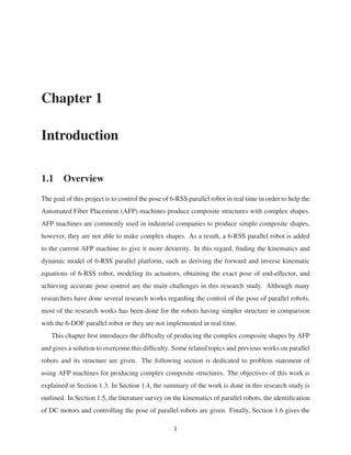
1.1 Frame with complex structure . . . . . . . . . . . . . . . . . . . . . . . . . . . . 2
1.2 Impossible for AFP to manufacture bicycle frame . . . . . . . . . . . . . . . . . . 3
1.3 Two possible solutions to improve AFP Machines . . . . . . . . . . . . . . . . . . 3
1.4 Parallel robot available in Concordia . . . . . . . . . . . . . . . . . . . . . . . . . 4
1.5 AFP available in Concordia . . . . . . . . . . . . . . . . . . . . . . . . . . . . . . 5
2.1 Entertainment device for movie theater [1]. . . . . . . . . . . . . . . . . . . . . . 18
2.2 Parallel robots . . . . . . . . . . . . . . . . . . . . . . . . . . . . . . . . . . . . . 19
2.3 Flight simulator [2] . . . . . . . . . . . . . . . . . . . . . . . . . . . . . . . . . . 19
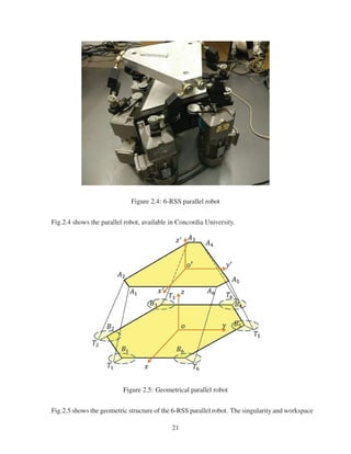
2.4 6-RSS parallel robot . . . . . . . . . . . . . . . . . . . . . . . . . . . . . . . . . 21
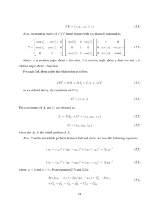
2.5 Geometrical parallel robot . . . . . . . . . . . . . . . . . . . . . . . . . . . . . . 21
2.6 The schematic representation of forward and inverse kinematics. . . . . . . . . . . 23
2.7 Kinematics model . . . . . . . . . . . . . . . . . . . . . . . . . . . . . . . . . . . 27
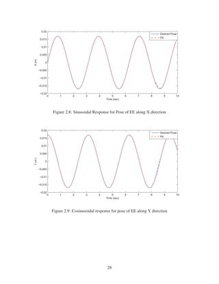
2.8 Sinusoidal Response for Pose of EE along X direction . . . . . . . . . . . . . . . . 28
2.9 Cosinusoidal response for pose of EE along Y direction . . . . . . . . . . . . . . . 28
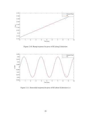
2.10 Ramp response for pose of EE along Z direction . . . . . . . . . . . . . . . . . . . 29
2.11 Sinusoidal response for pose of EE about X direction (α) . . . . . . . . . . . . . . 29
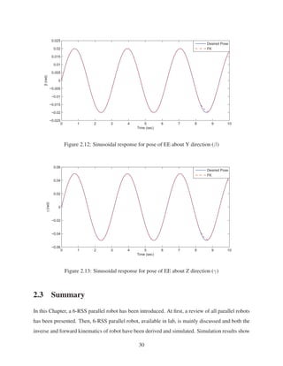
2.12 Sinusoidal response for pose of EE about Y direction (β) . . . . . . . . . . . . . . 30
2.13 Sinusoidal response for pose of EE about Z direction (γ) . . . . . . . . . . . . . . 30
3.1 Equivalent electrical circuit of a DC brushless motor [3]. . . . . . . . . . . . . . . 36
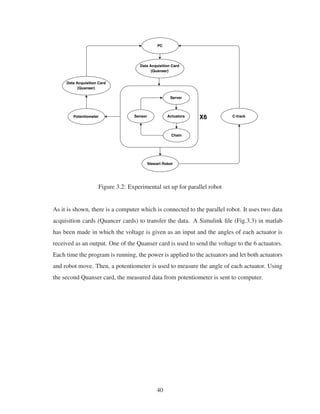
3.2 Experimental set up for parallel robot . . . . . . . . . . . . . . . . . . . . . . . . 40
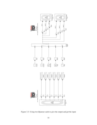
3.3 Using two Quanser cards to give the output and get the input . . . . . . . . . . . . 41
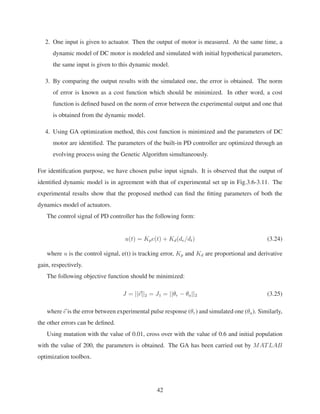
3.4 Comparing real motor model with the identified model using PD controller . . . . 43
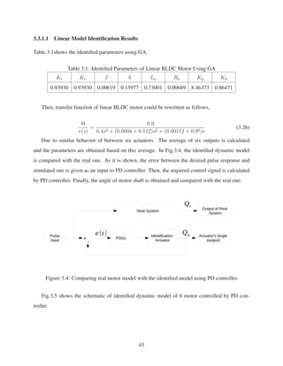
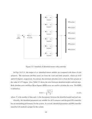
3.5 Simulink of identified motor with controller . . . . . . . . . . . . . . . . . . . . . 44
viii

9. 3.6 Pulse response and absolute error for first motor . . . . . . . . . . . . . . . . . . . 45
3.7 Pulse response and absolute error for second motor . . . . . . . . . . . . . . . . . 45
3.8 Pulse response and absolute error for third motor . . . . . . . . . . . . . . . . . . 46
3.9 Pulse response and absolute error for forth motor . . . . . . . . . . . . . . . . . . 46
3.10 Pulse response and absolute error for fifth motor . . . . . . . . . . . . . . . . . . . 46
3.11 Pulse response and absolute error for sixth motor . . . . . . . . . . . . . . . . . . 47
3.12 2-norm Level diagram of Pareto front of objective functions, J1 and J2 . . . . . . . 49
3.13 Sinusoidal response and absolute error for first motor . . . . . . . . . . . . . . . . 50
3.14 Sinusoidal response and absolute error for second motor . . . . . . . . . . . . . . 50
3.15 Sinusoidal response and absolute error for third motor . . . . . . . . . . . . . . . . 50
3.16 Sinusoidal response and absolute error for forth motor . . . . . . . . . . . . . . . . 51
3.17 Sinusoidal response and absolute error for fifth motor . . . . . . . . . . . . . . . . 51
3.18 Sinusoidal response and absolute error for sixth motor . . . . . . . . . . . . . . . . 51
3.19 Pulse response and absolute error for first motor . . . . . . . . . . . . . . . . . . . 52
3.20 Pulse response and absolute error for second motor . . . . . . . . . . . . . . . . . 52
3.21 Pulse response and absolute error for third motor . . . . . . . . . . . . . . . . . . 52
3.22 Pulse response and absolute error for forth motor . . . . . . . . . . . . . . . . . . 53
3.23 Pulse response and absolute error for fifth motor . . . . . . . . . . . . . . . . . . . 53
3.24 Pulse response and absolute error for sixth motor . . . . . . . . . . . . . . . . . . 53
4.1 Schematic of proposed PID controller in simulation . . . . . . . . . . . . . . . . . 56
4.2 Open loop path tracking of parallel robot . . . . . . . . . . . . . . . . . . . . . . . 57
4.3 Sinusoidal response for pose of EE along X direction . . . . . . . . . . . . . . . . 58
4.4 Cosinusoidal response for pose of EE along Y direction . . . . . . . . . . . . . . . 58
4.5 Ramp response for pose of EE along Z direction . . . . . . . . . . . . . . . . . . . 59
4.6 Sinusoidal response for pose of EE about X direction (α) . . . . . . . . . . . . . . 59
4.7 Sinusoidal response for pose of EE about Y direction (β) . . . . . . . . . . . . . . 60
4.8 Sinusoidal response for pose of EE about Z direction (γ) . . . . . . . . . . . . . . 60
4.9 Schematic of proposed PID controller . . . . . . . . . . . . . . . . . . . . . . . . 61
4.10 Sinusoidal response for pose of EE along X direction . . . . . . . . . . . . . . . . 61
4.11 Cosinusoidal response for pose of EE along Y direction . . . . . . . . . . . . . . . 62
ix

10. 4.12 Ramp response for pose of EE along Z direction . . . . . . . . . . . . . . . . . . . 62
4.13 Sinusoidal response for pose of EE about X direction (α) . . . . . . . . . . . . . . 63
4.14 Sinusoidal response for pose of EE about Y direction (β) . . . . . . . . . . . . . . 63
4.15 Sinusoidal response for pose of EE about Z direction (γ) . . . . . . . . . . . . . . 64
4.16 Schematic of proposed controller in the presence of the noise . . . . . . . . . . . . 64
4.17 Sinusoidal response for pose of EE along X direction in presence of the noise . . . 65
4.18 Cosinusoidal response for pose of EE along Y direction in presence of the noise . . 65
4.19 Ramp response for pose of EE along Z direction . . . . . . . . . . . . . . . . . . . 66
4.20 Sinusoidal response for pose of EE about X direction (α) in presence of noise . . . 66
4.21 Sinusoidal response for pose of EE about Y direction (β) in presence of noise . . . 67
4.22 Sinusoidal response for pose of EE about Z direction (γ) in presence of noise . . . 67
4.23 Schematic of proposed PID controller in the presence of disturbance and noise . . . 68
4.24 Sinusoidal response for pose of EE along X direction in the presence of disturbance
and noise . . . . . . . . . . . . . . . . . . . . . . . . . . . . . . . . . . . . . . . 68
4.25 Cosinusoidal response for pose of EE along Y direction in the presence of distur-
bance and noise . . . . . . . . . . . . . . . . . . . . . . . . . . . . . . . . . . . . 69
4.26 Ramp response for pose of EE along Z direction in the presence of disturbance and
noise . . . . . . . . . . . . . . . . . . . . . . . . . . . . . . . . . . . . . . . . . . 69
4.27 Sinusoidal response for pose of EE about X direction (α) in the presence of distur-
bance and noise . . . . . . . . . . . . . . . . . . . . . . . . . . . . . . . . . . . . 70
4.28 Sinusoidal response for pose of EE about Y direction (β) in the presence of distur-
bance and noise . . . . . . . . . . . . . . . . . . . . . . . . . . . . . . . . . . . . 70
4.29 Sinusoidal response for pose of EE about Z direction (γ) in the presence of distur-
bance and noise . . . . . . . . . . . . . . . . . . . . . . . . . . . . . . . . . . . . 71
4.30 Sinusoidal response for pose of EE along x axis . . . . . . . . . . . . . . . . . . . 74
4.31 Cosinusoidal response for pose of EE along y axis . . . . . . . . . . . . . . . . . . 74
4.32 Ramp response for pose of EE along z axis . . . . . . . . . . . . . . . . . . . . . 75
4.33 Sinusoidal response for pose of EE about x axis (α) . . . . . . . . . . . . . . . . . 75
4.34 Sinusoidal response for pose of EE about y axis (β) . . . . . . . . . . . . . . . . . 76
4.35 Sinusoidal response for pose of EE about z axis (γ) . . . . . . . . . . . . . . . . . 76
x

11. 5.1 C-track parts . . . . . . . . . . . . . . . . . . . . . . . . . . . . . . . . . . . . . . 79
5.2 C-track parts . . . . . . . . . . . . . . . . . . . . . . . . . . . . . . . . . . . . . . 79
5.3 Capturing targets by two cameras simultaneously . . . . . . . . . . . . . . . . . . 79
5.4 Experimental setup for parallel robot . . . . . . . . . . . . . . . . . . . . . . . . . 81
5.5 Probe calibration . . . . . . . . . . . . . . . . . . . . . . . . . . . . . . . . . . . 83
5.6 Parallel robot . . . . . . . . . . . . . . . . . . . . . . . . . . . . . . . . . . . . . 84
5.7 Parallel robot model in VXelements software . . . . . . . . . . . . . . . . . . . . 87
5.8 Finding EE pose . . . . . . . . . . . . . . . . . . . . . . . . . . . . . . . . . . . 88
5.9 Aligning frame O x y z pose . . . . . . . . . . . . . . . . . . . . . . . . . . . . . 88
5.10 Visual basic model . . . . . . . . . . . . . . . . . . . . . . . . . . . . . . . . . . 89
5.11 Lenght of ATi . . . . . . . . . . . . . . . . . . . . . . . . . . . . . . . . . . . . . 90
5.12 Lenght of Lz . . . . . . . . . . . . . . . . . . . . . . . . . . . . . . . . . . . . . 91
5.13 Modifying LA . . . . . . . . . . . . . . . . . . . . . . . . . . . . . . . . . . . . . 92
5.14 Length of BTi . . . . . . . . . . . . . . . . . . . . . . . . . . . . . . . . . . . . . 92
5.15 Sinusoidal response for pose of the EE along X direction . . . . . . . . . . . . . . 93
5.16 Cosinusoidal response for pose of the EE along Y direction . . . . . . . . . . . . . 94
5.17 Sinusoidal response for pose of the EE along Z direction . . . . . . . . . . . . . . 94
5.18 Error X . . . . . . . . . . . . . . . . . . . . . . . . . . . . . . . . . . . . . . . . 95
5.19 Error Y . . . . . . . . . . . . . . . . . . . . . . . . . . . . . . . . . . . . . . . . 95
5.20 Error Z . . . . . . . . . . . . . . . . . . . . . . . . . . . . . . . . . . . . . . . . 96
5.21 Using serial port for communication . . . . . . . . . . . . . . . . . . . . . . . . . 97
5.22 COM1 block . . . . . . . . . . . . . . . . . . . . . . . . . . . . . . . . . . . . . 97
5.23 Stream Client Receiver block . . . . . . . . . . . . . . . . . . . . . . . . . . . . . 98
5.24 Normal mode . . . . . . . . . . . . . . . . . . . . . . . . . . . . . . . . . . . . . 99
5.25 External mode . . . . . . . . . . . . . . . . . . . . . . . . . . . . . . . . . . . . . 100
5.26 Normal and external modes . . . . . . . . . . . . . . . . . . . . . . . . . . . . . . 101
5.27 Stream Client Sender block . . . . . . . . . . . . . . . . . . . . . . . . . . . . . . 102
5.28 Stream Client Receiver block . . . . . . . . . . . . . . . . . . . . . . . . . . . . . 103
5.29 PID controller . . . . . . . . . . . . . . . . . . . . . . . . . . . . . . . . . . . . . 104
5.30 Sinusoidal response for pose of EE about X direction without controller . . . . . . 105
xi

12. 5.31 Cosinusoidal response for pose of EE along Y direction without controller . . . . . 106
5.32 Sinusoidal response for pose of EE along Z direction without controller . . . . . . 106
5.33 Sinusoidal response for pose of EE about X direction (α) without controller . . . . 107
5.34 Sinusoidal response for pose of EE about Y direction (β) without controller . . . . 107
5.35 Sinusoidal response for pose of EE about Z direction (γ) without controller . . . . 108
5.36 Sinusoidal response for pose of EE along X direction, using PI controller . . . . . 109
5.37 Cosinusoidal response for pose of EE along Y direction, using PI controller . . . . 109
5.38 Sinusoidal response for pose of EE along Z direction, using PI controller . . . . . . 110
5.39 Sinusoidal response for pose of EE about X direction (α), using PI controller . . . 110
5.40 Sinusoidal response for pose of EE about Y direction (β), using PI controller . . . 111
5.41 Sinusoidal response for pose of EE about Z direction (γ), using PI controller . . . . 111
xii

13. List of Tables
3.1 Identified Parameters of Linear BLDC Motor Using GA . . . . . . . . . . . . . . 43
3.2 Error of identified linear model . . . . . . . . . . . . . . . . . . . . . . . . . . . . 45
3.3 Three-objective optimization results . . . . . . . . . . . . . . . . . . . . . . . . . 48
3.4 Absolute error of identified nonlinear model . . . . . . . . . . . . . . . . . . . . . 54
3.5 RMS error of identified nonlinear model . . . . . . . . . . . . . . . . . . . . . . . 54
4.1 PID tuned by trial and error . . . . . . . . . . . . . . . . . . . . . . . . . . . . . . 56
4.2 Comparing the pose’ steady state error with and without PID controllers . . . . . . 71
4.3 Comparing the pose’ ITAE with and without PID controllers . . . . . . . . . . . . 72
4.4 PID tuned by GA . . . . . . . . . . . . . . . . . . . . . . . . . . . . . . . . . . . 73
4.5 The pose’error of each axis in presence of tuned PID controller . . . . . . . . . . . 73
5.1 Measuring LATi
by C-track . . . . . . . . . . . . . . . . . . . . . . . . . . . . . . 90
5.2 Measuring Lzi
by C-track . . . . . . . . . . . . . . . . . . . . . . . . . . . . . . . 91
5.3 Measuring LAi
by C-track . . . . . . . . . . . . . . . . . . . . . . . . . . . . . . 92
5.4 Measuring LBTi
by C-track . . . . . . . . . . . . . . . . . . . . . . . . . . . . . . 93
5.5 Inverse kinematic validation . . . . . . . . . . . . . . . . . . . . . . . . . . . . . 95
5.6 PI tuned by trial and error . . . . . . . . . . . . . . . . . . . . . . . . . . . . . . . 108
5.7 Comparing the pose’ steady state error with and without PI controllers . . . . . . . 112
5.8 Comparing the pose’ITAE with and without PI controllers . . . . . . . . . . . . . 112
5.9 Normalized ITAE of the EE’s pose in simulations . . . . . . . . . . . . . . . . . . 113
5.10 Normalized ITAE of the EE’s pose in experiments . . . . . . . . . . . . . . . . . . 113
xiii

14. Chapter 1
Introduction
1.1 Overview
The goal of this project is to control the pose of 6-RSS parallel robot in real time in order to help the
Automated Fiber Placement (AFP) machines produce composite structures with complex shapes.
AFP machines are commonly used in industrial companies to produce simple composite shapes,
however, they are not able to make complex shapes. As a result, a 6-RSS parallel robot is added
to the current AFP machine to give it more dexterity. In this regard, finding the kinematics and
dynamic model of 6-RSS parallel platform, such as deriving the forward and inverse kinematic
equations of 6-RSS robot, modeling its actuators, obtaining the exact pose of end-effector, and
achieving accurate pose control are the main challenges in this research study. Although many
researchers have done several research works regarding the control of the pose of parallel robots,
most of the research works has been done for the robots having simpler structure in comparison
with the 6-DOF parallel robot or they are not implemented in real time.
This chapter first introduces the difficulty of producing the complex composite shapes by AFP
and gives a solution to overcome this difficulty. Some related topics and previous works on parallel
robots and its structure are given. The following section is dedicated to problem statement of
using AFP machines for producing complex composite structures. The objectives of this work is
explained in Section 1.3. In Section 1.4, the summary of the work is done in this research study is
outlined. In Section 1.5, the literature survey on the kinematics of parallel robots, the identification
of DC motors and controlling the pose of parallel robots are given. Finally, Section 1.6 gives the
1

15. organization of this thesis and Section 1.7 gives the summary of this chapter.
1.2 Problem Statement
Recently, the increasing usage of composite structures, especially in aerospace industry, motivated
researchers to improve the flexibility and manufacturability of the Automated Fiber Placement
(AFP) machines. Before using AFP machines, the well-known method of manufacturing is handy-
lay-up which has serious disadvantages; the process is time consuming and the substantial amount
of materials waste. AFP machines have improved the methods of manufacture of composites in
terms of speed, repeatability, good compact and reduction of waste. However, the current AFP
machines are mainly designed for the manufacture of components having the shape of shallow
plates, shells and tubes with different cross sections such as circular and elliptical. Hence these
AFP machines need some modifications by adding more degree of freedom, because it is difficult
for AFP machines to produce complex shapes such as tubes with double curvature or with T-shapes
or Y shapes, tube with flanges and closed loop bicycle frames (see Fig.1.1 and Fig.1.2).
Figure 1.1: Frame with complex structure
2

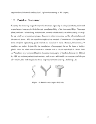
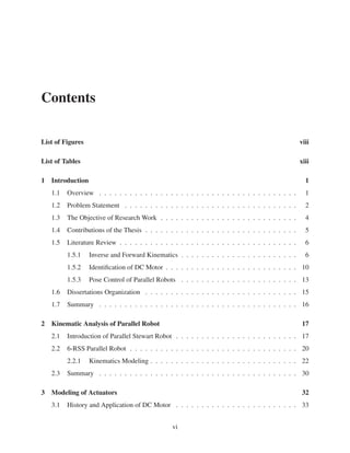
16. Figure 1.2: Impossible for AFP to manufacture bicycle frame
Two possible solutions are considered: One possible solution is to add a serial chain manipu-
lator to handle such complex structures. Unfortunately, serial robots incline to bend under heavy
loads and high speed which means that they could not carry heavy loads.
Another solution is to add 6-DOF parallel robots to the current AFP machines. Since 6-DOF
parallel robot provides high stiffness for a given structural mass, high accuracy and capability
of carrying heavy loads [4], it is an ideal mandrel holder for AFP to increase the flexibility of
composite manufacturing.
(a) Adding Serial Manipulator for Collaboration (b) Adding Hexapod for Collaboration
Figure 1.3: Two possible solutions to improve AFP Machines
3

17. To achieve this, a 6-RSS parallel robot, also called Stewart platform which is available in Con-
cordia University, has been added to the current AFP machine, in order to improve the performance
of the AFP machine to manufacturing of composite components.
1.3 The Objective of Research Work
The aim of this work is to add 6-RSS parallel robot to AFP machines in order to increase the
flexibility in manufacturing of composites. Therefore, obtaining the exact pose of the 6-DOF
parallel robot is necessary. To achieve this, the actuators’ model and the inverse kinematic model
of the parallel robot need to be built and identified. Then, C-track is applied to track the exact
pose of EE in real time. The pose obtained by C-track can be used to validate the derived inverse
kinematic model of the parallel robot.
Figure 1.4: Parallel robot available in Concordia
4

18. Figure 1.5: AFP available in Concordia
1.4 Contributions of the Thesis
The main contributions of the thesis are listed as follows
1. Both Inverse Kinematic (IK) and Forward Kinematic (FK) of 6-RSS parallel robot are ana-
lyzed. The IK model is derived using intractable problem between ball and circle, which is
required to control the parallel robot both in simulation and experiments. Since solving the
FK problem of 6-RSS parallel robot is complicated and produce multiple solutions, a simple
numerical method is used to solve the FK problem which gives us an unique answer. A FK
block is build in Simulink block diagram and it is used instead of real robot to gives us a pose
of the end-effector (EE). This FK block is used to control the pose of EE in simulations.
2. Both linear and nonlinear dynamic models of each actuator are derived through optimization
methods. First, the effect of friction is neglected and the parameters of the linear brushless
DC motor model are identified using Genetic Algorithm (GA). Then, the effect of friction
is considered and multi-objective optimization method is used to identify the parameters of
nonlinear brushless DC motor model.
3. Designing PID controller for the pose control of a 6-RSS parallel robot in simulation. In
order to control the pose of EE in simulation, both IK and FK blocks are used. The simulation
results indicated that the optimized PID controller tracks the pose of EE well.
5

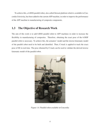
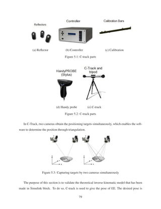
19. 4. Using C-track, the pose of EE is obtained in experimental works. Then the inverse kinemat-
ics of 6-RSS parallel robot is validated. In order to validate the inverse kinematic block, the
length of each link of parallel robot is calibrated. C-track is used for this calibration and the
links’ lengths are measured and substituted for links’ lengths measuring by ruler.
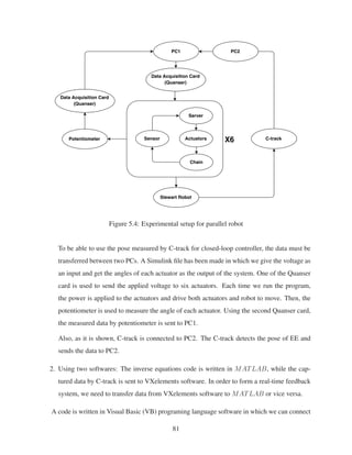
5. Two different PCs are used in the lab. One PC is connected to C-track and stores the
measured data from C-track. The other PC is connected to parallel robot and through two
Quanser cards we can control the robot. We succeed in transferring the data from the first
PC to the second one and running two Simulink models at the same time. This robot enables
us to have the feedback for pose control of the system.
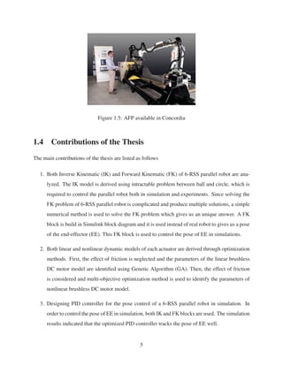
6. Six different PI controllers are designed to control the pose of EE in real time. Also, six low
pass filters are used to reduce the effect of noise. The experimental results show that these
PI controllers can track the desired pose at a satisfactory accuracy.
Also, the following lists are our publications during these two years:
• Alinia, S., Hemmatian, M., Xie, W.F. and Zeng, R., 2015, May. Posture control of
3-DOF parallel manipulator using feedback linearization and model reference adaptive
control. InElectrical and Computer Engineering (CCECE), 2015 IEEE 28th Canadian
Conference on(pp. 1145-1150). IEEE.
• Sahar Alinia, Amir Hajiloo, Wen-Fang Xie, Suong Hoa, 2015, Identification of the
dynamic model of 6 RSS parallel robots actuators. Poster IROS. IEEE
• Sahar Alinia, Wen-Fang Xie, Xiao-Ming Zhang. 2016, Modeling and pose control of a
6-RSS parallel robot using multi-objective optimization, CSME accepted
1.5 Literature Review
1.5.1 Inverse and Forward Kinematics
The analytical study of the robot’s motion without considering the forces is called kinematics
analysis which is classified into two parts [5]:
6

20. 1. Inverse Kinematic (IK): Inverse kinematics problem is expressed as determining the joint
variables of manipulator with respect to the given position and orientation of the EE.
2. Forward Kinematic (FK): Forward kinematics problem is defined as determining the pose of
EE with respect to base frame using given joint displacements.
In order to obtain the pose of parallel robot, analyzing the kinematics of robot is necessary. To
obtain the IK and FK of robots, two main challenges are considered:
• Number of degree of freedom (DOF): As the number of DOF is increased, deriving the
kinematic equations becomes more complicated.
• Types of robot: There are two types of robot, serial and parallel robots. In serial robots,
several series links connect the EE to the base. In contrast, the parallel robot is a robot in
which the base is connected to EE by several parallel links.
Depending on which kind of robot is studied, the complexity of obtaining the kinematics of
robot differs. For example, deriving the inverse kinematic equations of parallel robot is much
easier in comparison with that of serial robots. Whereas, deriving the forward kinematic
equations of parallel robot becomes very complicated. There is no unique solution when we
try to solve the FK equations of parallel robot. The more degree of freedom the robot has,
the more answers that the FK problem has.
There are two main methods to solve the FK problem, i.e., analytical and numerical methods. The
analytical method involves a lot of mathematic derivation and cannot give unique solution while
the second one calculates the pose of EE based on numerical techniques. Many studies have been
contributed to derive both inverse and forward kinematics of parallel robots.
1.5.1.1 Analytical Examples
In 1992, Shi et al.[6] presented a method to solve forward kinematic problem of 6-DOF Stewart
platform. This method was based on three point velocities of the end-effector. In this method, six
linear equations were solved. This method is easy to implement for the robot with six prismatic
joints.
7

21. Tsai et al.[7] solved the forward kinematics of 3 DOF parallel platform using Bezouts elim-
ination method in 2003. This method gave 64 possible solutions for FK problem. By applying
some physical limits, the sought solution could be obtained. Also, they proposed one optimization
method in order to find the pose of end-effector. This approach consumed less analysing time in
comparison with Bezouts elimination approach, because there was no need to calculate all possible
solutions. Also, Bezouts elimination approach might not be employed in real time applications due
to the optimization process and it was developed for 3 DOF Stewart robots.
Three years later, in 2007, Huang et al.[8] presented a novel method to solve the forward kine-
matics of 6-DOF Stewart robot. This method is called Algebraic Elimination which is convenient
for real time applications. In this algebraic method, they obtained the determinant of the 15x15
Sylvesters matrix in which 20th degree univariate polynomials were obtained. The proposed algo-
rithm could compute the forward kinematics in a short time and gave all the solutions briefly but
comprehensively. The obtained results by algebraic elimination method were confirmed by numer-
ical method. This method is used for general 6-DOF robots which consist of prismatic joints.
1.5.1.2 Numerical Examples
In 1991, Geng et al.[9] proposed the extended cascaded Cerebella Model Arithmetic Computer
(CMAC) structure based on the Neural Networks (NNs), in order to find the Forward Kinematic
(FK) of a Stewart platform. This extended CMAC network structure in comparison with a standard
single CMAC which had coarse and veneer nets. These coarse and veneer nets had different ranges
of input and output sensors which increased the faster learning ability of the complicated nonlinear
mappings. This means that the proposed method needed less time to be trained and could solve
the problem much faster than traditional FK solving methods. Also, they applied back propagation
algorithm to train NN in order to solve the FK problem. The comparison between Cascaded CMAC
and back propagation trained NNs, showed that the performance of the proposed method was more
ideal than the second one. This method was used in 1991 while other researchers proposed simple
numerical methods during last decade.
In 1993, Cleary et al.[10] used a numerical solution in order to solve the FK problem for 6-DOF
parallel platform. This method could be used in real time applications because of its high speed of
analysis. This method was used to solve a novel 6-DOF robot which is completely different from
8

22. 6-RSS robot.
At the same time, Liu et al.[11] presented a simple method in order solve the FK problem of
6-DOF general Stewart platform. Despite of many other algorithms which provided at least 30
equations, this method just gave three equations which should be solved at the same time. They
used Newton-Raphson method to solve these three equations. This method is used for the Stewart
platform having prismatic joints.
Three years later, McAree et al.[12] proposed an approach to solve the forward kinematic equa-
tions of Stewart platform. This method was based on Newton-Raphson scheme, which was very
robust and reliable in finding the FK solution. Also, this striking approach required short compu-
tational time and the performance was trustworthy, even though it faced with singularities. While
this methods is fast enough to solve the FK problem, Wang[13] proposed a numerical method later
which is simpler.
In 1997, Yee et al.[14] presented a novel neural network (NN) method in order to find the
forward kinematics (FK) solution of parallel manipulator (PM). Using inverse kinematic (IK) so-
lution, NN finds the solution by solving a series of nonlinear equations. A type of NN which was
used to solve FK equations is called feed-forward network. This proposed method was more pre-
cise than traditional NN ones. Although it took less time rather than the other NN methods, it is
still time consuming.
In 2002, Mu et al.[15] presented a numerical method based on polynomial continuation to solve
the FK problem for most Stewart platforms. They simplified a geometry of a real Stewart platform
to platform which was the start system. Instead of using pure mathematical equations, they used
start platform based on physical design. 18 second-order polynomial equations were developed
based on the distances between limbs connection points and limbs lengths. A homotopy was cre-
ated between the equations of real Stewart platform and start one. The parameters of start system
were changed into real ones using the created homotopy. With this homotopy, every obtained so-
lution for start system was tracked through a path in real space that led to find a complete set of
40 solutions for real platform. This method was verified through a numerical experiment and it is
used for general 6-DOF robots which consist of prismatic joints.
In 2006, Wang [13] presented a simple numerical method to solve FK problem of 6-DOF
parallel manipulators. This numerical method was based on trivial nature of inverse kinematics of
9

23. parallel platforms. Small changing in leg lengths led to small motion for robot. Using this, a linear
relationship between this two changes was derived. Then, a unique solution for FK problem was
obtained using a series of small leg lengths changes. This method was verified through numerical
examples.
In 2009, Parikh et al.[16] proposed an artificial neural network (ANN) method based on itera-
tive strategy to solve the FK problem. This method was useful in real time applications and gave
precise solutions. The comparison between the proposed method and single-layer ANN showed
that the more accurate solution could be obtained. Using the proposed method, the number of
iterations was less than five with acceptable error in terms of Stewart platform’s pose. Although
this method has accurate solution for FK problem it takes too much computational time.
In 2013, Morell et al.[17] proposed a spatial decomposition method to solve forward kinematics
of 6-DOF Stewart platform. This method did not depend on geometry of the Stewart platform. In
order to model the behavior of the platform in a given region of pose space, a famous machine
learning method was applied. This machine learning method is called the Support vector machines
(SVMs) which is used as a regression model in FK problem which is difficult to be implemented.
Solving the FK through numerical method is much faster. For our project, a simple numerical
method [13] is used to save the time and gives an accurate solution.
1.5.2 Identification of DC Motor
The basic structure of 6-RSS parallel robot, available in lab, includes 6 DC actuators serving as
actuators. Having the enough knowledge of these actuators is a crucial step towards analyzing the
behavior of the system.
The dynamic model of the actuators is usually classified into two categories:
• Linear model: This type of model only considers the force and motion in a straight line
which cause low frictional loss [18]. As a result, the dynamic equations of this motor could
be derived without considering the effect of friction.
• Nonlinear model: Mostly, the effect of friction is substantial in the motor, so friction force
must be considered when the dynamic model is derived. This type of model which considers
the friction force, is called nonlinear actuator’s model.
10

24. In order to operate, design and implement the motion control system for the actuator, both
static and dynamic mathematical models are required. These basic static and dynamic behaviors
are described by theoretical or physical modeling principles. Sometimes, the values of the required
parameters for modeling are not known. As a result, system identification is required to estimate
the parameters of the model. The identification of system dynamic model has been studied since
1960s [19].
In this thesis, in addition to the geometrical parameters of the robot, having the precise values
of the parameters of DC motor in order to control the system is required. The main challenge is
to consider the effect of friction. Considering the friction force in dynamic equation during the
identification, increases the processing time and makes system complicated. In this research, a
nonlinear DC motor model is identified using multi-objective optimization method to increase the
accuracy of identification.
Many researchers have carried out research in identifying both linear and nonlinear DC motors’
models and many papers have been published in this regard:
In 2004, Kara et al.[20] identified linear and nonlinear DC motor models. In order to identify
the nonlinear system model, a nonlinear Hammerstein structured was used. A discrete time ARX
model was used to identify the linear part. For nonlinear part, the Recursive Least Squares (RLS)
method was implemented. Although Hammerstein method was not able to be employed to con-
trol the online DC motor, it could identify the dead-zone features well. The experimental results
showed that the nonlinear model performed better than linear one for low speed process.
In 2005, Krneta et al.[21] identified parameters of DC motor using Recursive Least Squares
(RLS) method. In order to validate the experimental results, they used optical encoder to measure
the angles of motor. Comparing the speed of motor measured by optical encoder with the speed of
identified system, the identified parameters were matched with the real ones. They simulated the
identified model in computer and compared the real motor’s speed with the speed of identified one
in a Z and S domain. The simulations and experimental results showed a satisfactory identified
DC motor model. Two year later, Nasri et al. [22] presented a Particle Swarm Optimization (PSO)
method to identify the motor model and PID controller for a linear brushless DC motor. The
simulation results from PSO with GA and Linear Quadratic Regulator (LQR) method, shows the
better performance of optimized PID controller. The rise time, steady-state error, settling time and
11

25. maximum overshoot are reduced in this method in comparison to LQR and GA in addition to the
improved computational efficiency and easier implementation.
In 2007, Mamani et al.[23] presented an on-line, non-asymptotic, algebraic identification method
to identify the parameters of DC servo motor model. This method just depended on the input volt-
age and angular position of the motor so it does not need initial conditions. This method could
give the estimations in a short period of time. Also, the Coulombs friction coefficient of servo
motor was identified. Both high frequency noises and Coulomb friction torque were applied to the
system. The experimental results showed a good robustness of system in presence of noise and
friction.
In 2011, Peng et al.[24] identified a nonlinear DC motor system with dead-zone characteris-
tics. They modeled the DC motor using Wiener-type Neural Network (WNN). In order to control
the DC motor, PID-type Neural Network (PIDNN) was designed. Then, an adaptive PID-type
neural network control is proposed based on WNN. The designed controller is reported to have a
satisfactory performance.
At the same time, Bhushan et al.[25] identified and controlled the DC servo motor speed to
track the trajectory using Bacterial Forging Algorithm (BFA). The simulation results showed that
the designed adaptive controller tracked the desired trajectory very well. The estimated angular
speed of DC servo motor can approximate within a reasonable error. Also, they used GA based on
adaptive control to track the speed trajectory. Although the simulation results showed the speed
trajectorys error was less than that in BFA adaptive control, BFA adaptive controller needed less
computational time and works more efficiently.
At the same time, Wu [26] presented an identification method based on Tylor series expansion
of the motor speed response under a constant voltage input. This method could identify the pa-
rameters of DC motor such as, torque constant, electrical time constant, mechanical time constant
and friction. This approach was applied to modeling a Mabuchi RK370CA and Mabuchi FC130
motors. The systems were assessed under two conditions; with disturbance-torque and without
disturbance-torque. Then a model of motor has identified and verified bt the experimental results.
In 2014, Farid et al.[27] employed Particle Swarm Optimization (PSO) method to identify non-
linear DC motor model. Also, a controller was designed based on adaptive neuro-fuzzy inference
system. The control algorithm was implemented using Atmega32 microcontrollers. This method
12

26. decreased computational cost considerably. Also, the cheap microcontroller were used to realize.
The simulation results showed the satisfactory control.
Although many DC motor models have been identified so far using different methods, most
of them are based on simulation results. In this research both linear and nonlinear DC motor
models are identified using GA and multi objective optimization, respectively and are validated by
experimental results.
1.5.3 Pose Control of Parallel Robots
In addition to establishing kinematics models of the robot and identifying the parameters of robot’s
actuators, obtaining the exact pose of end-effector (EE) is necessary. Since the mandrel for fiber
layup is located on the EE of the parallel robot, the exact pose of EE must be determined for the
fiber placement. When the parallel robot is moving to the desired pose, it usually has some errors
which will affect the accuracy of fiber placement. To reduce this error, a controller should be used.
In this thesis, a set of PID controllers is used to control the pose of parallel robot in real time. There
are several papers are published regarding linear and nonlinear pose control of parallel robots. The
main challenge lies in controlling the pose of 6-RSS parallel robot simultaneously in real time.
Six controllers should be tuned to deliver a satisfactory pose tracking performance. The second
challenge is that we have to apply these controllers in experiments which is a very demanding and
needs excessive effort.
Some researches have been reported in the literature regarding the pose control of parallel
robot:
In 2004, Huang et al.[28] presented a sliding mode control method to control the motion of 6-
DOF Stewart platform with some parametric uncertainties. The only measurable parameters were
the positions and velocities of the links. These types of controller were model-based and require
the dynamic model of Stewart platform. They derived important dynamic properties of the system.
The experimental results indicated an outstanding performance for the designed controller.
In 2005, Huang and Fu [29] controlled the motion of Stewart platform using a smooth sliding
mode control method. The only measurable parameters were the positions and velocities of the
links while other parameters are subjected to uncertainties. These types of controller are model-
based and require the dynamic model of Stewart platform. They derived the important dynamic
13

27. properties of the system. They analyzed the stability of system using Lyapunov theory and showed
that the controller was stable.
In 2006, Sun et al.[30] proposed a cross-coupled control approach for synchronous control
of 3-DOF Stewart platform. Comparing with most of the synchronous controller, this controller
was easy to implement because the explicit knowledge of dynamic model of the system was not
required. In this paper, this synchronous control was compared with two other controllers, i.e.,
conventional PID and adaptive controllers. The experimental results showed that the proposed
controller had smaller position error of EE and the smaller position errors of the three prismatic
joints.
Zhu et al.[31] presented a discontinuous projection-based adaptive robust control strategy for
a 3-DOF parallel manipulator driven by pneumatic muscles. The time-varying friction forces and
the static force dynamic modeling errors of pneumatic muscles caused harsh parametric uncer-
tainties and uncertain nonlinearities for the system. The proposed controller was used to reduce
these nonlinearities and uncertainties. Both simulation and experimental results showed the pro-
posed adaptive controller tracked the desired pose accurately. Also, they presented an adaptive
robust control (ARC) to control the pose of a parallel manipulator driven by pneumatic muscles
(PMDPM) with a redundant DOF. The experimental results showed a precise pose tracking control
for the system.
In the same year, Zhao et al.[32] developed a fully adaptive feedforward feedback synchro-
nized tracking controller for a 6-DOF Stewart platform. There had been an error between the
obtained feedforward control gains and real parameters. The error effects were compensated using
the saturated controller. They compared the proposed controller with two other controllers, i.e.,
PID controller and synchronized controller (A-S) control. The simulation results showed that the
proposed controller and A-S control tracked the desired pose well and has less error than PID con-
troller. The dynamic structure of Stewart platform is very complicated. The advantage of proposed
controller is that could be implemented without any knowledge of the dynamic structure of Stew-
art platform while A-S controller was model-based controller. As a result, this proposed controller
was easier to be implemented and more applicable in practice rather than A-S one.
In 2011, Bo et al.[33] presented a control algorithm based on fuzzy logic and PID control algo-
rithms. The designed controller is tested on experimental setup. Both simulation and experimental
14

28. results showed that the designed controller tracked the pose of Stewart platform precisely.
Also, Jian et al.[34] proposed a control method which is based on Narendras model reference
adaptive control method. The simulation and experimental results showed a satisfactory perfor-
mance of the proposed controller.
In 2012, Srikanth et al.[35] presented a mathematical model of a three-phase BLDC motor.
Then, two PID controllers were designed using GA and Ziegler Nichols method (ZN). Although
ZN was effectively used to estimate the initial values of PID gains in GA, the simulation results
showed the better performance of the controller tuned by GA. The performance index, such as the
rise time, settling time, overshoot of the controller tuned by GA were reduced in comparison with
that of the tuned controller by ZN.
In 2015, Alinia et al.[36] designed two model-based controllers (i.e. feedback linearizion and
model reference adaptive controls (MRAC)) for a 3-DOF parallel manipulator driven by pneu-
matic muscles (PMDPM). Two controllers were developed to control the pose of moving platform
by changing the pressure inside the pneumatic muscles. The simulation results showed the sat-
isfactory tracking performance of the designed controllers under sudden disturbances and their
robustness against the noise. The MRAC exhibited better control performance compared with
feedback linearizion controller.
Above literature survey shows that a lot of research in the pose control of the parallel platforms.
However, most of the controllers are not implemented in real time. Also, many of the controlled
robots have less than 6 DOFs. This project aims at controlling the pose of 6-RSS parallel robot
in real time. To do so, some experiments have been done which is very time consuming and
challenging. The results show the satisfactory pose tracking of the EE’s pose.
1.6 Dissertations Organization
This work has been organized as follows: In the following chapter, the definition of the 6-RSS
parallel robot, R stands for revolute joint and S for spherical joint, which is available in Concordia
University, is presented. Then, the inverse kinematic equations of the 6-RSS parallel robot, is ob-
tained. Moreover, based on the inverse kinematic model, an appropriate direct kinematic solution
is required to obtain the EE’s pose of the parallel robot, theoretically.
15

29. In order to simulate with the parallel robot for pose controller design, in Chapter 3, the linear
brushless DC actuators’ models are identified. Also, the nonlinear brushless DC motor model
and corresponding dynamic equations are given. Then, GA is used to identify the parameters of
nonlinear brushless DC motor model. Moreover, the multi-objective optimization method using
GA is selected to identify the parameters of nonlinear DC actuator model considering the friction.
Then, a PID controller is used to control the actuators and the gains of the PID controller are tuned
by using GA.
In Chapter 4, a C-track is used to obtain the pose of EE. The parallel robot is modeled in VX-
elements provided by C-track, and the inverse kinematic model is verified. Then, the data obtained
by the C-track is transfered from one PC to another one by using the serial port. In order to control
the pose of EE, the obtained pose by C-track is compared with the desired pose and the pose error
is input to the controller. Finally, the thesis is concluded and future work is provided in Chapter 5.
1.7 Summary
In this chapter, a brief introduction of basic concepts of the current research has been presented.
A literature review on the existing works on the kinematics analysis of model identification of DC
motor and pose control of parallel robots has been given. The information on research objectives
and the thesis organization are also given in this chapter.
16

30. Chapter 2
Kinematic Analysis of Parallel Robot
To design the pose controller for the parallel robot in simulation, it is necessary to conduct the
kinematic analysis of the robot for simulating the robot. Both inverse and forward kinematic
equations are required for pose control in the simulations. The forward kinematic model will
be combined with the dynamic model of the actuators to mimic the parallel robot behavior and
the pose information output of the parallel robot can be obtained from this model to serve as the
feedback signal for closed-loop pose control system. While the inverse kinematic model can be
used to generate the command to the actuators in the simulation. The main objective of this chapter
is to derive the kinematics of 6-RSS parallel robot in order to control the pose of EE. The accuracy
of these equation are validated experimentally in the following chapters.
This chapter is organized as follows: In Section 2.1, the parallel robots are introduced and
a brief history of parallel robots is given. In Section 2.2, 6-RSS-DOF parallel robot, which is
available in Concordia university, is described. Then, the inverse and forward kinematics of 6-RSS
parallel robot are obtained and modeled in Simulink block diagram.
2.1 Introduction of Parallel Stewart Robot
Nowadays, robot manipulators are commonly used in manufacturing industry to fulfill different
tasks, such as spray painting, spot welding, lifting different parts with different mass, assembling,
etc[37]. There are two types of robots which are widely used in industrial applications. The first
one is called parallel robot and the second one is known as a serial robot.
17

31. Parallel robot is a kind of robot built with closed-loop chains. Using at least two kinematic
chains, the base is connected to EE. A kinematic chain consists of several links which are linked
by joints. In overall, parallel robot is defined as a mechanism in which the base is connected to
EE through several chains. A serial manipulator is a robot built with an open-loop chain structure,
which means that only one path connects each link to other link.
The main difference between serial robots and parallel manipulators is their structure. In serial
robots the base is connected to EE through several series links, while in parallel robots the base
and EE are linked by a number of parallel linkages.
The origin of Stewart parallel platform dates back to 1920s, when French and English mathe-
maticians were interested in polyhedral. The first parallel robot was invented by James Gwinnet
in 1928. He invented a 3-RRR parallel robot as an entertainment device for movie theater (see
Fig.2.1) [1].
Figure 2.1: Entertainment device for movie theater [1].
As it is shown in Fig.2.2 (a), Willard L.V.Pollard invented a parallel robot for spray painting and
controls the position of a spray gun, in 1940 and 1942 respectively [38], [39]. A 6-DOF parallel
robot is designed by Eric Gough in 1947 where the industry is hit by such invention [40] (see
Fig.2.2 (b)). This well-known robot is called universal machine and is used in tire inspection. In
1965, Stewart presented a 6-DOF parallel robot which was different from Goughs parallel platform.
This robot is used as a flight simulator (see Fig.2.3) and made an evolution in both industry and
academic research [2]. In 1967, Klaus Cappel, proposed a motion simulator hexapod which made
him the third pioneer in the field of parallel robots.
18

32. (a) Spray painting robot [38] and [39]. (b) Tire inspection robot [40].
Figure 2.2: Parallel robots
Figure 2.3: Flight simulator [2]
Due to the following features, parallel robots are widely used in industries application where
the conventional serial robots have some limitations:
• Higher stiffness: They provide higher stiffness for a given structural mass in comparison
with the serial manipulators [41].
• Strong load bearing: Parallel robots are able to carry heavy loads; therefore, they are used as
flight simulator, automobile simulator, tank simulator, earthquake simulator and so on [4].
• Satisfying dynamic performance: They have high velocity and acceleration for pick-and-
place concept, such as delta robots [42].
19

33. • Less accumulated errors of joints: In serial robots, the errors accumulate because the links
are series, while in parallel robot the errors of parallel links are averaged [43]. It is used as
micro-manipulators or manipulator for ophthalmic surgery operation where the high accurate
positioning is required [4], [43].
• Simpler inverse kinematics. The inverse kinematic equations of parallel robots are much
easier than serial robots which makes them more suitable for real time application [1].
• They are used in many other applications such as, Neuro-surgical robot [44], optical fiber
alignment [45], and so on.
However, there are some drawbacks in the parallel robot, such as;
• Small workspace: The work space of parallel robot is much less than that of serial robots.
Finding the work space of parallel robots, also, is more difficult than that of serial ones [1].
• Complex dynamic model: It is difficult to find the dynamic equation for parallel robots [40].
• Complex forward kinematic model: It is very complicated to find the unique solution to
forward kinematic equations of parallel robot. So, many researchers tried to find the unique
solution to the FK equations by using numerical methods [40].
2.2 6-RSS Parallel Robot
As it mentioned in Chapter 1, the aim of using 6-RSS parallel robot is to add more dexterity to the
current AFP machines. Therefore, obtaining the exact pose of the parallels EE is necessary. The
current 6-RSS robot, available in Concordia University, and its features are given in this section.
20

34. Figure 2.4: 6-RSS parallel robot
Fig.2.4 shows the parallel robot, available in Concordia University.
Figure 2.5: Geometrical parallel robot
Fig.2.5 shows the geometric structure of the 6-RSS parallel robot. The singularity and workspace
21

35. analysis have been given in [46]. This robot consists of the following parts:
• A moving platform which has translations of motion along x-y-z axes and three rotations
around all axes.
• A base platform which is fixed.
• 6 rotary actuators which are DC brushless motors.
• 6 links (ATi) and 6 links (BTi), (i = 1, 2...6).
As it is shown in the figure, two frames (Oxyz and O x y z ) are considered in which the frame
Oxyz is fixed to base platform and used as the reference frame, and the frame O x y z is attached
to the moving platform. The posture of the EE is defined as the rotating angles around x by
role angle (α), y axis by pitch angle (β), z axis by yaw angle (γ), respectively. Also, there are
translations along x, y and z directions. Bi is a revolute joint and the location of actuators. BTi
linkages are located in x-y which rotates about Bi in z direction. Ai and Ti are spherical joints
which let the moving platform has three rotations and translations along three axes.
2.2.1 Kinematics Modeling
Kinematics studies the motion of bodies without considering the forces or moment that causes the
motion. In other word, the analytical study of the motion of robot represents robot kinematics.
Formulating suitable kinematics modeling of the manipulator is very crucial for analyzing the
behavior of industrial manipulators [5].
The robot kinematics includes forward kinematics and inverse kinematics.
1. Inverse Kinematics: Determination of joint variables in respect of end-effector position and
orientation is called inverse kinematics. To control the end-effector to reach a pose, the
inverse kinematic must be built.
2. Forward Kinematics: Calculating the position and orientation of the end-effector according
to the joint variables is called forward kinematics. To simulate the parallel robot for pose
control design purpose, the forward kinematics model must be built as well.
22

36. Solving inverse kinematic equation of parallel manipulators is straightforward while for serial
manipulators is very complex and time taking. In contrast, forward kinematics problem of serial
manipulators is easy to be solved whereas for parallel manipulator, solving forward kinematics
problem is very challenging. It is computationally expensive and requires a lot of mathematic
derivations. Some difficulties should be considered while deriving forward kinematic equations
especially when the structure of manipulator is complicated. The more degree of freedom the
robot has, the more complex manipulator’s structure becomes. This complexity causes multiple
solutions and singularities.
The relationship between forward and inverse kinematics is illustrated in Fig.2.6.
Figure 2.6: The schematic representation of forward and inverse kinematics.
There are two main methods to solve forward kinematics, analytical and numerical methods.
In the first method, a lot of mathematics derivations are required. In the second one, calculating
the position and orientation of the end-effector are obtained based on the numerical techniques.
Compared with the analytical method, the numerical method is faster and accurate enough when
the structure of robot is complex, i.e., the robot has 6 DOFs [5].
2.2.1.1 Inverse Kinematic Modeling of 6-RSS Robot
The determination of joint variables from end-effector’s position and orientation is called inverse
kinematics. To control the end-effector to reach a desired pose, the inverse kinematic equations
must be solved.
In this section, the inverse kinematics equation of 6 DOF-RSS parallel robot is presented.
The position of EE with respect to the coordinate of O in xyz frame, is defined as follows:
23

37. EE = (x, y, z, α, β, γ) (2.1)
Also, the rotation matrix of x y z frame respect with xyz frame is obtained as,
R =
⎡
⎢
⎢
⎢
⎣
cos(γ) −sin(γ) 0
sin(γ) cos(γ) 0
0 0 1
⎤
⎥
⎥
⎥
⎦
⎡
⎢
⎢
⎢
⎣
cos(β) 0 sin(β)
0 1 0
−sin(β) 0 cos(β)
⎤
⎥
⎥
⎥
⎦
⎡
⎢
⎢
⎢
⎣
1 0 0
0 cos(α) −sin(α)
0 sin(α) cos(α)
⎤
⎥
⎥
⎥
⎦
(2.2)
where, α is rotation angle about x direction, β is rotation angle about y direction and γ is
rotation angle about z direction.
For each link, there exists the relationship as follow,
OO = OBi + BiTi + TiAi + AiO (2.3)
as we defined above, the coordinate of O is:
O = (x, y, z) (2.4)
The coordinates of Ai and Bi are obtained as,
Ai = RA0,i + O = (xAi
, yAi
, zAi
) (2.5)
Bi = (xBi
, yBi
, zBi
) (2.6)
where the A0,i is the initial position of Ai.
Also, from the intractable problem between ball and circle, we have the following equations:
(xTi
− xAi
)2
+ (yTi
− yAi
)2
+ (zTi
− zAi
)2
= (LAT )2
(2.7)
(xTi
− xBi
)2
+ (yTi
− yBi
)2
+ (zTi
− zBi
)2
= (LBT )2
(2.8)
where, zt = a and zb = 0. From equation(2.7) and (2.8):
2xTi
(xBi
− xAi
) + 2yTi
(yBi
− yAi
) + z2
Ai
− 2azAi
+x2
Ai
+ y2
Ai
− x2
Bi
− y2
Bi
= L2
AT − L2
BT
(2.9)
24

38. Then one has:
xTi
=
N1
2(xAi
− xBi
)
−
yAi
− yBi
xAi
− xBi
yTi
(2.10)
where N1 is defined as follows:
N1 = −L2
AT + L2
BT + (x2
Ai
+ y2
Ai
) − (x2
Bi
+ y2
Bi
)
+zAi
(zAi
− 2a)
(2.11)
Substituting xTi
from equation (2.10), in equation (2.8) yields:
N2y2
Ti
+ 2N3yTi
+ N4 = 0 (2.12)
Therefore, yTi
is obtained as follows:
yTi
=
−N3 + N2
3 − 4N2N4
2N2
(2.13)
or
yTi
=
−N3 − N2
3 − 4N2N4
2N2
(2.14)
where, N2, N3 and N4 can be described as follows:
N2 =
(yAi
− yBi
)2
(xAi
− xBi
)2
+ 1 (2.15)
N3 = −2
(yAi
− yBi
)
(xAi
− xBi
)
[
N1
2(xAi
− xBi
)
− xBi
] − 2yBi
(2.16)
N4 = (
N1
2(xAi
− xBi
)
− xBi
)2
− L2
BT + y2
Bi
+ z2
Ti
(2.17)
When N2
3 − 4N2N4 ≥ 0, the desired pose is available. Furthermore, when the range of θ is
between [−π, π], the solution for yTi
is unique.
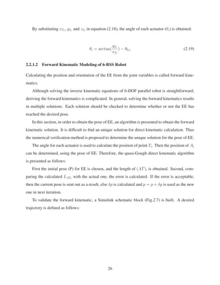
Furthermore, there is a relationship between the coordinate of Ti and the rotation angle of each
actuator (θi) as follows:
⎡
⎢
⎢
⎢
⎣
xTi
yTi
zTi
⎤
⎥
⎥
⎥
⎦
=
⎡
⎢
⎢
⎢
⎣
cos(θi + θ0,i) −sin(θi + θ0,i) 0
sin(θi + θ0,i) cos(θi + θ0,i) 0
0 0 1
⎤
⎥
⎥
⎥
⎦
⎡
⎢
⎢
⎢
⎣
LTB
0
0
⎤
⎥
⎥
⎥
⎦
(2.18)
25

39. By substituting xTi
, yTi
and zTi
in equation (2.18), the angle of each actuator (θi) is obtained:
θi = arctan(
yTi
xTi
) − θ0,i (2.19)
2.2.1.2 Forward Kinematic Modeling of 6-RSS Robot
Calculating the position and orientation of the EE from the joint variables is called forward kine-
matics.
Although solving the inverse kinematic equations of 6-DOF parallel robot is straightforward,
deriving the forward kinematics is complicated. In general, solving the forward kinematics results
in multiple solutions. Each solution should be checked to determine whether or not the EE has
reached the desired pose.
In this section, in order to obtain the pose of EE, an algorithm is presented to obtain the forward
kinematic solution. It is difficult to find an unique solution for direct kinematic calculation. Thus
the numerical verification method is proposed to determine the unique solution for the pose of EE.
The angle for each actuator is used to calculate the position of point Ti. Then the position of Ai
can be determined, using the pose of EE. Therefore, the quasi-Gough direct kinematic algorithm
is presented as follows:
First the initial pose (P) for EE is chosen, and the length of (AT)i is obtained. Second, com-
paring the calculated LATi
with the actual one, the error is calculated. If the error is acceptable,
then the current pose is sent out as a result, else δp is calculated and p = p + δp is used as the new
one in next iteration.
To validate the forward kinematic, a Simulink schematic block (Fig.2.7) is built. A desired
trajectory is defined as follows:
26

40. x = 0.017sin(2t) (2.20)
y = 0.017cos(2t) (2.21)
z = 0.1185 + (0.2/250)t (2.22)
α = 0.02sin(2t) (2.23)
β = 0.02sin(2t) (2.24)
γ = 0.05sin(2t) (2.25)
where, t is time (sec), x, y, z are the position of EE (m) and α, β and γ are rotations about x, y, z
axises (rad), respectively.
In Fig.2.7, the desired trajectory is inputted to inverse kinematic block which gives us six
angles. Then, these angles is fed to forward kinematic block to obtain the pose of EE. This pose
are supposed to be as same as desired trajectory we give to inverse kinematic equations.
Figure 2.7: Kinematics model
Fig2.8-Fig2.13 show the desired trajectory and the calculated pose by forward kinematics.
Comparing desired pose with the pose which is obtained by FK model, it proves that IK and FK
model have an agreement with each other.
27

41. 0 1 2 3 4 5 6 7 8 9 10
−0.02
−0.015
−0.01
−0.005
0
0.005
0.01
0.015
0.02
Time (sec)
X(m)
Desired Pose
FK
Figure 2.8: Sinusoidal Response for Pose of EE along X direction
0 1 2 3 4 5 6 7 8 9 10
−0.02
−0.015
−0.01
−0.005
0
0.005
0.01
0.015
0.02
Time (sec)
Y(m)
Desired Pose
FK
Figure 2.9: Cosinusoidal response for pose of EE along Y direction
28

42. 0 1 2 3 4 5 6 7 8 9 10
0.118
0.119
0.12
0.121
0.122
0.123
0.124
0.125
0.126
0.127
Time (sec)
Z(m)
Desired Pose
FK
Figure 2.10: Ramp response for pose of EE along Z direction
0 1 2 3 4 5 6 7 8 9 10
−0.025
−0.02
−0.015
−0.01
−0.005
0
0.005
0.01
0.015
0.02
0.025
Time (sec)
α(rad)
Desired Pose
FK
Figure 2.11: Sinusoidal response for pose of EE about X direction (α)
29

43. 0 1 2 3 4 5 6 7 8 9 10
−0.025
−0.02
−0.015
−0.01
−0.005
0
0.005
0.01
0.015
0.02
0.025
Time (sec)
β(rad)
Desired Pose
FK
Figure 2.12: Sinusoidal response for pose of EE about Y direction (β)
0 1 2 3 4 5 6 7 8 9 10
−0.06
−0.04
−0.02
0
0.02
0.04
0.06
Time (sec)
γ(rad)
Desired Pose
FK
Figure 2.13: Sinusoidal response for pose of EE about Z direction (γ)
2.3 Summary
In this Chapter, a 6-RSS parallel robot has been introduced. At first, a review of all parallel robots
has been presented. Then, 6-RSS parallel robot, available in lab, is mainly discussed and both the
inverse and forward kinematics of robot have been derived and simulated. Simulation results show
30

44. that forward kinematics and inverse kinematic model are agreed with each other.
31

45. Chapter 3
Modeling of Actuators
Having acquiring the knowledge about the kinematics of 6-RSS parallel robot, we want to inves-
tigate the dynamic behavior of the actuators. Six actuators consist of six brush-less DC motors.
Inverse kinematic block gives a desired set of angles (θ1, θ2, ...θ6) corresponding to a specific pose.
These angles are input to the actuators (Motor1, Motor2, ...Motor6). Then, the actuators are con-
trolled to move to the desired angles and the current angle of each one of them (output of each
motor) is obtained by potentiometer. A experimental setup is made to measure the output of ac-
tuators. These outputs are input to the forward kinematic block which mimic the motion of the
parallel robot. To do so, in addition to the IK and FK models of the parallel robot, finding the
parameters of each actuator’s dynamic model is required. These actuators’ model parameters are
identified using optimization methods and the dynamic model of each actuator is built. For pose
control design of the robot, the outputs of the actuators with the simulated dynamic models are
compared and the identified model is validated.
The goal of this chapter is to identify the parameters of six actuators model. In this regards,
a brief history of BLDC motor is discussed in Section 3.1. Then, in Section 3.2, both linear and
nonlinear dynamic models of BLDC motor are represented. In Section 3.3, the experimental setup
is described and the parameters of proposed linear model are identified using GA. Moreover, a
nonlinear dynamic model of BLDC motor is proposed and identified using multi-objective opti-
mization method. Finally, the identified dynamic models are verified in experiments.
32

46. 3.1 History and Application of DC Motor
Generally, DC motors consist of an armature which rotates. The armature consists of three main
parts: shaft, core and copper winding inserted in slots. These parts determine the main features
of DC motor including bearing life, brush life, Electromagnetic Interference (EMI), and acoustical
noise.
Due to the excellent speed control over acceleration and deceleration with effective and simple
torque control (speed control over a wide range both above and below the rated speed), DC motor
has been popularly used in industrial even though it has some crucial drawbacks as well [47]; for
example:
• Replacing the brushes: Brushes should be replaced frequently because of sliding contact
between commutator and brushes slides, since this contact causes wear problem.
• Producing electrical interference: Brushes and commutator have electrical contact which
might cause electromagnetic interference[48]. This electrical interference makes noise. One
solution is to use filter in order to remove the noise, however it cannot completely prevent to
make the undesirable noise.
• Flashing: This electrical interference between commutator and brushes causes DC motor
sparks which is dangerous in corrosive conditions.
• High initial cost: For better communication, the winding inductance is to be kept at a mini-
mum. Increasing the number of armature coils is the solution to improve the communication
for the conventional DC motors. Considering the cost, this solution is not a practical. In-
stead of this, the moving-coil version of the DC motor is the same as the toothless version of
the brushless motor which has low inductance, low electrical time constant, and minimum
magnetic drag.
In order to avoid these deficits, another type of DC motor has been invented which is called
brushless DC motor (BLDC). The DC motor is replaced by BLDC motor which has the similar
features in comparison with conventional DC motor, except it does not have brushes and commuta-
tor part. Because the brushes not only need regular maintenance, but also introduce wear problems
33

47. which impose sparking, undesirable noise and speed limitations.
The BLDC motor usually consist of a permanent magnet rotor which rotates about armatures,
a number of fixed stator windings around the rotor, entire sensing system, and electronic switch-
ing circuits. This new structure increases the torque speed in comparison with conventional DC
motor[49].
The field flux is supplied by the permanent magnets which are mounted on the rotor and are
arranged in pole pairs. The stator is designed in such a way that if the current reaches the coils at
a right time, the interaction with the field flux occurs and toque is produced. An absolute sensing
system is required to locate magnets which is necessary for the coil to be switched in the correct
sequence and at a correct time. The electronic commutator takes the information from the sensors
and processes it to switch the currents in the stator coils.
Generally, it has many advantages such as simple maintenance, low price and reliability. Also,
they are easy to be constructed [50]. BLDC motor provides variable speed operation. These motors
are used in high performance motion control products, such as machine tools. These advantages
make an increase in interest in the use of this kind of motor [51].
The DC motor has been widely used in industry because of the excellent speed control over
acceleration and deceleration with effective and simple torque control (speed control over a wide
range both above and below the rated speed) [52].
The classical model of DC motor is a linear second-order equation one which is discussed in
following section.
3.2 Dynamic Modeling
As it is mentioned before, BLDC motors are usually utilized in industrial applications due to
the stable and straight forward characteristics associated with them [53]. As a result, finding the
dynamic model for DC motor has attracted many researchers’ attention and methods have been
proposed. In this section linear BLDC motor model is adopted and identified by using GA. The
linear model neglects the effect of friction. As a result, a nonlinear BLDC motor model is presented
and identified using multi-objective optimization method in Section 3.3.
34

48. 3.2.1 Linear Model
In general, the torque generated by a DC motor is proportional to the armature current and the
strength of magnetic field [54]. The magnetic field is assumed to be constant. Therefore, the
motor torque is proportional to only the armature current i by a constant factor Kt as shown in the
equation below,
T = Kti (3.1)
the back emf, e, is proportional to the angular velocity of the shaft by an electromotive force
constant Ke.
e = Ke
˙θ (3.2)
In SI units, the motor torque and back emf constants are equal, therefore, Kt = Ke = K.
Based on Newtons second law and Kirchhoff’s voltage law, the following equations are derived,
J ¨θ + b ˙θ = Ki (3.3)
La
di
dt
+ Rai = V − Ke
˙θ (3.4)
where, J is the moment of inertia of the rotor (Kg.m2
), b is the motor viscous friction constant
(N.m.s), La is electric inductance (H), Ra is the electric resistance (Ohm).
Applying the Laplace transform, the above modeling equations can be explained in terms of
the Laplace variables.
J(s2
)Θ + bsΘ = KI (3.5)
LsI + RI = V − KsΘ (3.6)
I =
(V − KsΘ)
(Ls + R)
(3.7)
(3.8)
By eliminating I(s) between two above equations, the transfer function of DC motor is obtained
as follows:
Js2
Θ + bsΘ = K
V − KsΘ
Ls + R
(3.9)
Θ(Js2
+ bs)(Ls + R) = KV − K2
sθ (3.10)
KV = Θ(JLs3
+ JRs2
+ bLs2
+ bRs) + K2
sΘ (3.11)
35

49. So, the transfer function of DC motor obtained as follows:
Θ
V
=
K
JLs3 + (JR + bL)s2 + (bR + K2)s
(3.12)
where, R = Ra is armature resistance, (Ω), L = La is armature inductance, (H), v is Armature
voltage, (V ), e(t) is back emf voltage, (V ), Kb is back emf constant, (V/(rad/sec)), K = Kt is
torque constant, (N.m/A), Tm is torque developed by the motor, (N.m), Θ(t) is angular displace-
ment of shaft, (rad), J is moment of inertia of motor and load, (Kg-m2
/rad), and b is motor viscous
friction constant, (N.m.s).
The linear model neglects nonlinear friction which causes negative effects on the systems per-
formance. The nonlinear friction models and their identification for DC motor will be built and
identified in following section [20], [3], [55], [53].
3.2.2 Nonlinear Model
As it is mentioned, before the linear DC motor model neglects the dead zone of motor that has a
great effect on the system of motor [3]. In order to improve the accuracy of the model, the effect
of nonlinear friction is considered in DC modeling. Considering the nonlinear friction model, the
friction torque applied to the system results in the DC motor model which becomes a second-order
nonlinear model.
An equivalent electrical circuit of BLDC is represented in Fig.3.1.
Figure 3.1: Equivalent electrical circuit of a DC brushless motor [3].
The torque balance equation of DC motor can be described as follows,
J ˙ω + Bω = Kti (3.13)
36

50. where, J is the inertia moment of the rotor (kg.m2
), Kt is the torque coefficient of DC motor
(N.m/A), and B is viscous friction coefficient of DC motor (N.m.s/rad). The linear DC motor is
given by,
J ˙ω + Bω = Kti (3.14)
La˙ı =V − Keω − Raı (3.15)
y = ω (3.16)
Consider the torque introduced by the friction,
Bω + J ˙ω + Tcsgn(ω) = Kti − f(ω) (3.17)
La˙ı = V − Keω − Raı (3.18)
y = ω (3.19)
where, f(ω) is friction and could be defined as,
f(ω) = (Ts − Tc)exp(−α.|ω|)sign(ω) (3.20)
where, Tc is the Coulomb friction torque (N.m), Ts is static friction torque (N.m), α is time
constant, ω is the angular velocity of the actuator (rad/s).
By dividing both sides of the equation (3.17) by J, and also both sides of the Eq.(3.18) by La,
Eqs. (3.21) and (3.22) could be rewritten as,
˙ω = −K1ω − K2sgn(ω) − K3exp(−K4|ω|)sgn(ω)
+K5i
(3.21)
˙ı = K6V − K7ω − K8ı (3.22)
37

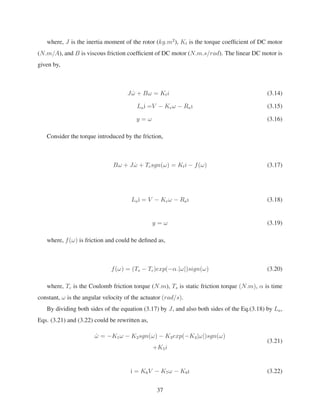
51. y = ω (3.23)
where, K1 = B/J, K2 = Kt/J, K3 = Ra/La, K4 = Ke/La, K5 = 1/La, K6 = Tc/J, K7 =
(Ts − Tc)/J, K8 = α, K = [K1, K2, K3, K4, K5, K6, K7, K8]T
is the parameter vector that con-
tains eight parameters. In next few sections, these parameters are identified by multi-objective
optimization using GA.
In the following section, the identification of both linear and nonlinear DC motor models are
discussed.
3.3 Parameters’ Identification
In order to achieve the collaboration operation between parallel robot and AFP machines, obtaining
the exact pose of 6-RSS parallel robot is necessary. To achieve this, a proper dynamic model of
each actuator is required. There are plenty of identification methods to obtain the parameters of
actuators. Among all of them, GA is employed in this work study to identify the DC motor model’s
parameters.
The aim of Section 3.3.1 is to identify the dynamic model of linear DC motor without consid-
ering effect of friction. First, an experimental setup is built to measure the output of each actuator.
Then, GA is used to identify the parameters of linear DC motor model.
In the Section 3.3.2, to obtain the parameters of nonlinear DC motor, GA was applied first;
but the result was not satisfactory. It was due to the nonlinear friction which is not considered in
the linear model. Using only GA to optimize just one objective function for parameter identifica-
tion, cannot find the nominal parameters. Usually, there is not one objective but there are several
ones which should be optimized, i.e. costs, time, reliability and performance [56]. In fact, these
objectives are sometimes even in conflict with each other. These problems can be considered as
multi-objective problems (MOPs). Accordingly, multi-objective optimization method is used to
find trade-offs among objectives [57]. GA is one of the most efficient means to solve MOPs, due
to its unity and universal aspects. In order to solve this problem, multi-objective method is applied
to optimize two objective functions for the nonlinear model identification at the same time.
38

52. 3.3.1 Parameters’ Identification Using Genetic Algorithm
The history of GA dates back to 1970s where John Holland introduced and developed the GA
based evolutionary ideas of natural selection [58].
In this method, the population of the candidate solution is evolved towards a better solution.
The procedure is listed as follows:
1. A random population of chromosomes is generated.
2. Then the fitness of each chromosome is evaluated.
3. New population is created based on selection, crossover and mutation.
4. Finally the old population is replaced by new generated population. The goodness of solution
is typically defined with respect to the current population [59].
GA has its advantages, for example: Every optimization problem could be solved in which the
chromosomes encoding can be described. Also the problem with multiple solutions could be solved
by GA. Moreover, multidimensional, non-differential, non-continuous and even non-parametrical
problems can be solved since this method is not dependent on the error surface [59].
Besides its advantages, there are several disadvantages as well [60]. There is no absolute
insurance that the global optimum will be found. It happens very often when the populations have
a lot of subjects. Like other artificial intelligence techniques, the genetic algorithm cannot assure
the constant optimization response time. Due to this property, the usage of GA will be limited
in real time application. In this section, GA is applied to find the optimized parameters of the
dynamic model of the DC actuators. To collect the data for identification we have retrofitted the
controller of the parallel robot with two Quanser Cards.
The identification procedure is shown as follows:
1. First, an experimental set up is built to measure the angles of the Stewart’s (the robot) motors.
Fig.3.2 is the set up for our experiment work:
39

53. Figure 3.2: Experimental set up for parallel robot
As it is shown, there is a computer which is connected to the parallel robot. It uses two data
acquisition cards (Quancer cards) to transfer the data. A Simulink file (Fig.3.3) in matlab
has been made in which the voltage is given as an input and the angles of each actuator is
received as an output. One of the Quanser card is used to send the voltage to the 6 actuators.
Each time the program is running, the power is applied to the actuators and let both actuators
and robot move. Then, a potentiometer is used to measure the angle of each actuator. Using
the second Quanser card, the measured data from potentiometer is sent to computer.
40

54. Figure 3.3: Using two Quanser cards to give the output and get the input
41

55. 2. One input is given to actuator. Then the output of motor is measured. At the same time, a
dynamic model of DC motor is modeled and simulated with initial hypothetical parameters,
the same input is given to this dynamic model.
3. By comparing the output results with the simulated one, the error is obtained. The norm
of error is known as a cost function which should be minimized. In other word, a cost
function is defined based on the norm of error between the experimental output and one that
is obtained from the dynamic model.
4. Using GA optimization method, this cost function is minimized and the parameters of DC
motor are identified. The parameters of the built-in PD controller are optimized through an
evolving process using the Genetic Algorithm simultaneously.
For identification purpose, we have chosen pulse input signals. It is observed that the output of
identified dynamic model is in agreement with that of experimental set up in Fig.3.6-3.11. The
experimental results show that the proposed method can find the fitting parameters of both the
dynamics model of actuators.
The control signal of PD controller has the following form:
u(t) = Kpe(t) + Kd(de/dt) (3.24)
where u is the control signal, e(t) is tracking error, Kp and Kd are proportional and derivative
gain, respectively.
The following objective function should be minimized:
J = ||e||2 = J1 = ||θr − θa||2 (3.25)
where e is the error between experimental pulse response (θr) and simulated one (θa). Similarly,
the other errors can be defined.
Using mutation with the value of 0.01, cross over with the value of 0.6 and initial population
with the value of 200, the parameters is obtained. The GA has been carried out by MATLAB
optimization toolbox.
42

56. 3.3.1.1 Linear Model Identification Results
Table.3.1shows the identified parameters using GA.
Table 3.1: Identified Parameters of Linear BLDC Motor Using GA
Kt Ke J b La Ra Kp Kd
0.93930 0.93930 0.00619 0.15977 0.73001 0.00689 8.46373 0.86471
Then, transfer function of linear BLDC motor could be rewritten as follows,
Θ
v(s)
=
0.9
0.4s3 + (0.0004 + 0.112)s2 + (0.00112 + 0.92)s
(3.26)
Due to similar behavior of between six actuators. The average of six outputs is calculated
and the parameters are obtained based on this average. In Fig.3.4, the identified dynamic model
is compared with the real one. As it is shown, the error between the desired pulse response and
simulated one is given as an input to PD controller. Then, the required control signal is calculated
by PD controller. Finally, the angle of motor shaft is obtained and compared with the real one.
Figure 3.4: Comparing real motor model with the identified model using PD controller
Fig.3.5 shows the schematic of identified dynamic model of 6 motor controlled by PD con-
troller.
43

57. Theta_Motor2
Theta_Motor6
Theta_Motor5
Theta_Motor3
Theta_Motor1
Theta_Motor4
Subsystem5
In1 Out1
Subsystem4
In1 Out1
Subsystem3
In1 Out1
Subsystem2
In1 Out1
Subsystem1
In1 Out1
Subsystem
In1 Out1
Pulse
Generator
PD Controller
PD(s)
Figure 3.5: Simulink of identified motor with controller
In Figs.3.6-3.11, the output of six identified motors models are compared with those of real
actuators. The maximum absolute errors are from the sixth and forth actuators, which are 6.82
and 6.52 degrees, respectively. In contrast, the minimum absolute error is from the first actuator at
the value of 4.37 degree. Also, Table.3.2 shows the error between identified models and real ones.
Both absolute error and Root Mean Square (RMS) error are used to calculate the error. The RMS
is defined as,
RMS =
N
1
2
N
(3.27)
where N is the number of data and is the discrepancy between the identified model and real one.
Overally, the identified parameters are suitable for all 6 actuators and designed PD controller
has an outstanding performance for the system. As a result, identified parameters and PD controller
tuned by GA method is proper for the system.
44

58. Table 3.2: Error of identified linear model
Error of Actuators (θ) Pulse response(deg) RMS(deg)
First Actuator 4.374 0.5389
Second Actuator 5.77 0.7834
Third Actuator 4.976 0.6865
Forth Actuator 6.52 0.9032
Fifth Actuator 5.7 0.8333
Sixth Actuator 6.82 0.9479
0 2 4 6 8 10 12 14 16 18 20
0
5
10
15
20
25
30
Time (sec)
θ1
(deg)
First Actuator (θ1
)
Simulated Actuator
0 2 4 6 8 10 12 14 16 18 20
0
0.1
0.2
0.3
0.4
0.5
0.6
0.7
Time (sec)
ErrorofFifthActuator(δθ
5
)(a) Pulse response for first motor (b) Absolute error of θ1
Figure 3.6: Pulse response and absolute error for first motor
0 2 4 6 8 10 12 14 16 18 20
0
5
10
15
20
25
30
Time (sec)
θ2
(deg)
Second Actuator (θ
2
)
Simulated Actuator
0 2 4 6 8 10 12 14 16 18 20
0
1
2
3
4
5
6
Time (sec)
ErrorofSecondActuator(δθ
2
)(deg)
(a) Pulse response for second motor (b) Absolute error of θ2
Figure 3.7: Pulse response and absolute error for second motor
45

59. 0 2 4 6 8 10 12 14 16 18 20
0
5
10
15
20
25
30
Time (sec)
θ3
(deg)
Third Actuator (θ3
)
Simulated Actuator
0 2 4 6 8 10 12 14 16 18 20
0
1
2
3
4
5
6
Time (sec)
ErrorofThirdActuator(δθ
3
)(deg)
(a) Pulse response for third motor (b) Absolute error of θ3
Figure 3.8: Pulse response and absolute error for third motor
0 2 4 6 8 10 12 14 16 18 20
0
5
10
15
20
25
30
Time (sec)
θ4
(deg)
Forth Actuator (θ
4
)
Simulated Actuator
0 2 4 6 8 10 12 14 16 18 20
0
1
2
3
4
5
6
7
Time (sec)
ErrorofForthActuator(δθ
4
)(deg)
(a) Pulse response for forth motor (b) Absolute error of θ4
Figure 3.9: Pulse response and absolute error for forth motor
0 2 4 6 8 10 12 14 16 18 20
0
5
10
15
20
25
30
Time (sec)
θ5
(deg)
Fifth Actuator (θ
5
)
Simulated Actuator
0 2 4 6 8 10 12 14 16 18 20
0
1
2
3
4
5
6
Time (sec)
ErrorofFifthActuator(δθ
5
)
(a) Pulse response for fifth motor (b) Absolute error of θ5
Figure 3.10: Pulse response and absolute error for fifth motor
46

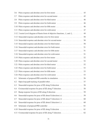
60. 0 2 4 6 8 10 12 14 16 18 20
0
5
10
15
20
25
30
Time (sec)
θ6
(deg)
Sixth Actuator (θ6
)
Simulated Actuator
0 2 4 6 8 10 12 14 16 18 20
0
1
2
3
4
5
6
7
Time (sec)
ErrorofSixthActuator(δθ
6
)(deg)
(a) Pulse response for sixth motor (b) Absolute error of θ6
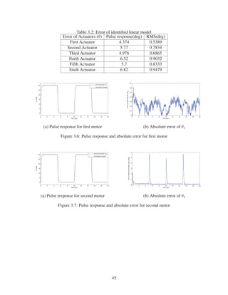
Figure 3.11: Pulse response and absolute error for sixth motor
3.3.2 Parameters’ Identification Using Multi-objective
The purpose of this section is to identify dynamic model of DC motor considering friction effect
for 6-RSS platform using multi-objective optimization.
Most of the engineering problems have more than one objective functions which should be op-
timized, i.e. minimizing the cost, maximizing the performance and reliability. Since, the objective
functions often conflict with each other, and improving one of them may deteriorate the others[61].
A set of solutions, so called, Pareto fronts are obtained so that a reasonable set of solutions satis-
fying all objective functions at an acceptable level without being dominated by any other solution
[62],[63].
Multi-objective optimization, also called multicriteria optimization or vector optimization has
been defined as finding a vector of decision variables satisfying the constraints to give accept-
able values to all objective functions[62]. In general, it can be defined as finding a set of values
[x∗
1, x∗
2, . . . , x∗
n] to optimize k objectives or cost functions [f1(x), f2(x), . . . , fk(x)] with giving
x = [x1, x2, . . . , xn]T
, which is the n-dimensional decision variable vector in the solution space X.
Among many approaches, GA is the most popular one to optimize multi-objective problems
[64]. GA is used to find a set of multiple non-dominated solutions in a single run. Searching
different regions of solution space by GA at the same time, leads to finding various set of solutions
for difficult problems with non-convex, discontinuous, and multi-modal solutions spaces.
In this work, multi-objective using GA is used to find the parameters of the model of the DC
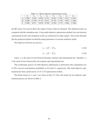
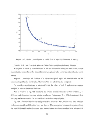
actuators. The identification procedure is shown as follows. The following two objective functions
(3.27 and 3.28) are defined, which should be minimized. Two different input voltages are given to
47

61. Table 3.3: Three-objective optimization results
K1 K2 K3 K4 K5 K6 K7 K8
A 0.998 0.350 0.030 0.741 18.827 5.547 4.933 12.447
B 0.986 0.3199 0.119 0.613 18.791 4.349 4.965 11.606
C 0.980 0.071 0.030 0.498 15.585 3.153 4.460 11.080
the DC motor. For each of them, the output of motor shaft are obtained. The obtained results are
compared with the simulation ones. Using multi-objective optimization method, the error between
experimental results and simulation results are minimized for input signals. Our results illustrate
that the proposed method can find the proper parameters of actuator nonlinear model.
The objective functions are given as,
J1 = ||θP
e − θP
s ||2 (3.28)
J2 = ||θS
e − θS
s ||2 (3.29)
where J1 is the norm of error between the pulse response and experimental one. Similarly, J2
is the norm of error between the sine response and experimental one.
The evolutionary process of multi-objective optimization is performed with a population size
of 250, crossover and mutation probability as 0.8 and 0.1, respectively. The multi-objective opti-
mization has been carried out by MATLAB optimization toolbox.
The Pareto fronts of J1 and J2 are shown in Fig.3.12 Also, the results for two-objective opti-
mization process are shown in Table 2.
48

62. J2
0.2 0.3 0.4 0.5 0.6 0.7 0.8 0.9 1 1.1
J1
0.8
1
1.2
1.4
1.6
1.8
2
2.2
2.4
2.6
A
B
C
Figure 3.12: 2-norm Level diagram of Pareto front of objective functions, J1 and J2
Consider A, B , and C as three points on Pareto front, which have following features:
A is a point in which J2 is minimum but J1 has the worst value among the other values, which
means that the norm of error for sinusoidal input has optimal value but for pulse input has the worst
values.
At point C, although, the value of J1 is optimal for pulse input, the norm of error for the
sinusoidal input has the worst value. Therefore, C is not selected as the best point.
For point B, which is chosen as a trade off point, the values of both J1 and J2 are acceptable
and give us a set of reasonable solutions.
As it is observed in Fig.3.12, point B is the optimal point in which the system with the J1 =
1.22 can track the desired response with the small error. Furthermore, J2 = 0.54 shows an excellent
tracking performance and it can be considered as the best trade-off point.
Fig.3.14-3.18 show the sinusodial response of six actuators. Also, the absolute error between
real motors models and identified ones are shown. The comparison between the response from
the identified models and real actuator ones, shows that the maximum absolute error is from sixth
49

63. motor with the value of 0.74 degree while the minimum absolute error is from the first actuator
actuator with 0.62 degree.
0 2 4 6 8 10 12 14 16 18 20
−30
−20
−10
0
10
20
30
Time (sec)
θ1
(deg)
First Actuator (θ
1
)
Simulated Actuator
0 2 4 6 8 10 12 14 16 18 20
0
0.1
0.2
0.3
0.4
0.5
0.6
0.7
Time (sec)
ErrorofFirstActuator(δθ
1
)(deg)
(a) Sinusoidal response (b) Absolute error
Figure 3.13: Sinusoidal response and absolute error for first motor
0 2 4 6 8 10 12 14 16 18 20
−30
−20
−10
0
10
20
30
Time (sec)
θ
2
(deg)
Second Actuator (θ
2
)
Simulated Actuator
0 2 4 6 8 10 12 14 16 18 20
0
0.1
0.2
0.3
0.4
0.5
0.6
0.7
0.8
Time (sec)
ErrorofSecondActuator(δθ
2
)(deg)
(a) Sinusoidal response (b) Absolute error
Figure 3.14: Sinusoidal response and absolute error for second motor
0 2 4 6 8 10 12 14 16 18 20
−30
−20
−10
0
10
20
30
Time (sec)
θ
3
(deg)
Third Actuator (θ
3
)
Simulated Actuator
0 2 4 6 8 10 12 14 16 18 20
0
0.1
0.2
0.3
0.4
0.5
0.6
0.7
Time (sec)
ErrorofThirdActuator(δθ
3
)(deg)
(a) Sinusoidal response (b) Absolute error
Figure 3.15: Sinusoidal response and absolute error for third motor
50

64. 0 2 4 6 8 10 12 14 16 18 20
−30
−20
−10
0
10
20
30
Time (sec)
θ4
(deg)
Forth Actuator (θ4
)
Simulated Actuator
0 2 4 6 8 10 12 14 16 18 20
0
0.1
0.2
0.3
0.4
0.5
0.6
0.7
0.8
Time (sec)
ErrorofForthActuator(δθ
4
)(deg)
(a) Sinusoidal response (b) Absolute error
Figure 3.16: Sinusoidal response and absolute error for forth motor
0 2 4 6 8 10 12 14 16 18 20
−30
−20
−10
0
10
20
30
Time (sec)
θ
5
(deg)
Fifth Actuator (θ
5
)
Simulated Actuator
0 2 4 6 8 10 12 14 16 18 20
0
0.1
0.2
0.3
0.4
0.5
0.6
0.7
Time (sec)
ErrorofFifthActuator(δθ
5
)
(a) Sinusoidal response (b) Absolute error
Figure 3.17: Sinusoidal response and absolute error for fifth motor
0 2 4 6 8 10 12 14 16 18 20
−30
−20
−10
0
10
20
30
Time (sec)
θ
6
(deg)
Sixth Actuator (θ
6
)
Simulated Actuator
0 2 4 6 8 10 12 14 16 18 20
0
0.1
0.2
0.3
0.4
0.5
0.6
0.7
Time (sec)
ErrorofSixthActuator(δθ
6
)(deg)
(a) Sinusoidal response (b) Absolute error
Figure 3.18: Sinusoidal response and absolute error for sixth motor
Figs.3.19-3.24 show the pulse response of six actuators. Also, the absolute error between the
response of real motors and identified ones are shown. The comparison between the responses
shows that the maximum absolute error is from the sixth one with the value of 4.34 degree while
the minimum absolute error is from the first actuator with 2.30 degree.
51

65. 0 2 4 6 8 10 12 14 16 18 20
0
5
10
15
20
25
30
Time (sec)
θ1
(deg)
First Actuator (θ1
)
Simulated Actuator
0 2 4 6 8 10 12 14 16 18 20
0
0.5
1
1.5
2
2.5
3
3.5
4
4.5
Time (sec)
ErrorofFirstActuator(δθ
1
)(deg)
(a) Pulse response (b) Absolute error
Figure 3.19: Pulse response and absolute error for first motor
0 2 4 6 8 10 12 14 16 18 20
0
5
10
15
20
25
30
Time (sec)
θ2
(deg)
Second Actuator (θ2
)
Simulated Actuator
0 2 4 6 8 10 12 14 16 18 20
0
0.5
1
1.5
2
2.5
Time (sec)
ErrorofSecondActuator(δθ
2
)(deg)
(a) Pulse response (b) Absolute error
Figure 3.20: Pulse response and absolute error for second motor
0 2 4 6 8 10 12 14 16 18 20
0
5
10
15
20
25
30
Time (sec)
θ3
(deg)
Third Actuator (θ3
)
Simulated Actuator
0 2 4 6 8 10 12 14 16 18 20
0
0.5
1
1.5
2
2.5
3
Time (sec)
ErrorofThirdActuator(δθ
3
)(deg)
(a) Pulse response (b) Absolute error
Figure 3.21: Pulse response and absolute error for third motor
52

66. 0 2 4 6 8 10 12 14 16 18 20
0
5
10
15
20
25
30
Time (sec)
θ4
(deg)
Forth Actuator (θ4
)
Simulated Actuator
0 2 4 6 8 10 12 14 16 18 20
0
0.5
1
1.5
2
2.5
3
Time (sec)
ErrorofForthActuator(δθ
4
)(deg)
(a) Pulse response (b) Absolute error
Figure 3.22: Pulse response and absolute error for forth motor
0 2 4 6 8 10 12 14 16 18 20
0
5
10
15
20
25
30
Time (sec)
θ5
(deg)
Fifth Actuator (θ5
)
Simulated Actuator
0 2 4 6 8 10 12 14 16 18 20
0
0.5
1
1.5
2
2.5
Time (sec)
ErrorofFifthActuator(δθ
5
)(deg)
(a) Pulse response (b) Absolute error
Figure 3.23: Pulse response and absolute error for fifth motor
0 2 4 6 8 10 12 14 16 18 20
0
5
10
15
20
25
30
Time (sec)
θ6
(deg)
Sixth Actuator (θ6
)
Simulated Actuator
0 2 4 6 8 10 12 14 16 18 20
0
0.5
1
1.5
2
2.5
3
Time (sec)
ErrorofSixthActuator(δθ
6
)(deg)
(a) Pulse response (b) Absolute error
Figure 3.24: Pulse response and absolute error for sixth motor
Table.3.4 and Table.3.5 show the error of each actuator for both pulse response and sinusoidal
responses:
Overall, the identified model are accurate to represent the dynamic behavior of all 6 actuators
and the designed PD controller can match the built-in controller in the six actuators’ model. As a
53

67. Table 3.4: Absolute error of identified nonlinear model
Pulse response(deg) Sinusoidal response (deg)
First actuator 2.3 0.62
Second actuator 2.415 0.70
Third actuator 2.7 0.63
Forth actuator 2.84 0.73
Fifth actuator 2.2 0.61
Sixth actuator 4.34 0.74
Table 3.5: RMS error of identified nonlinear model
Pulse response(deg) Sinusoidal response (deg)
First actuator 0.7005 0.3130
Second actuator 0.5608 0.2771
Third actuator 0.5149 0.2379
Forth actuator 0.5537 0.3340
Fifth actuator 0.4997 0.2426
Sixth actuator 0.5644 0.3208
result, the identified parameters of nonlinear model tuned by multi-objective optimization method
is proper for simulating actuators for the pose controller design in the next chapter.
3.4 Summary
In this chapter a brief history of DC motor has been presented. An experimental set up for par-
allel robot and its actuators, has been presented. Both linear and nonlinear DC motors have been
proposed and modeled. The parameters of linear DC motor model have been identified using GA
method. The results of the obtained dynamic model have been compared with experimental ones
and proved an accurate modeling for the linear DC motors. Considering the effect of friction, the
parameters of nonlinear DC motor have been identified using multi-objective optimization. The
accuracy of the identified dynamic model of each actuator is validated in experiment.
54

68. Chapter 4
Pose Control
This chapter is devoted to pose control of the 6-RSS parallel robot. After obtaining IK and FK of
the parallel robot and the dynamic nonlinear model of the actuators, we can simulate the parallel
robot and design a pose controller in the simulation. The IK can generate the desired angles for
PID pose controller from the pose error and FK is used to simulate the parallel kinematic motion
and generate the pose as the feedback for pose controller.
4.1 Controlling the Pose of EE in Presence of Linear BLDC
Motor Model
This section, the control pose of EE is discussed. Fig.4.1 shows the schematic of the proposed
controller. As it can be seen in this figure, the error between the desired pose and the simulated
one is given as an input to the inverse block. Then, δθ goes to the controller to obtain the control
signal which is required by the actuators. In this study, the forward kinematic model is used to get
a feedback from EE.
In order to control the system, a PID controller is used in this study. The design of these
controllers is based on three parameters: proportional gain, integral time constant and derivative
time constant. The control signal of PID controller has the following form:
u(t) = Kpe(t) + Ki e(t)dt + Kdd(e(t)/dt) (4.1)
55

69. Table 4.1: PID tuned by trial and error
Kp Ki Kd
12 100 0.2
where u is the control signal, e(t) is tracking error, Kp, Ki, and Kd are proportional, integral,
and derivative gain, respectively.
Figure 4.1: Schematic of proposed PID controller in simulation
Table.4.1 shows the gains of tuned PID controller by trial and error.
Also, the control of the pose of EE in presence of noise and disturbance are discussed. First,
the open loop system is built in the Simulink block diagram in which the desired pose trajectory
is given to inverse kinematics. Then, the obtained angles by the inverse kinematic model are fed
to the motor model. Finally, the obtained angles from the motor are fed to the forward kinematic
model and the results are compared to the desired ones (Fig.4.2).
56

70. Figure 4.2: Open loop path tracking of parallel robot
In order to evaluate the performance of the controller, a desired trajectory is defined as follows:
x = 0.007sin(2t) (4.2)
y = 0.007cos(2t) (4.3)
z = 0.1185 + 0.2t/250 (4.4)
α = 0.02sin(2t) (4.5)
β = 0.02sin(2t) (4.6)
γ = 0.05sin(2t) (4.7)
where, t is time (sec), x, y, z are the position of EE (mm) and α, β and γ are rotations about x, y,
z axises (rad), respectively.
57

71. 0 1 2 3 4 5 6 7 8 9 10
−8
−6
−4
−2
0
2
4
6
8
x 10
−3
Time (sec)
X(m)
Desired
Simulated
Figure 4.3: Sinusoidal response for pose of EE along X direction
0 1 2 3 4 5 6 7 8 9 10
−8
−6
−4
−2
0
2
4
6
8
x 10
−3
Time (sec)
Y(m)
Desired
Simulated
Figure 4.4: Cosinusoidal response for pose of EE along Y direction
58

72. 0 1 2 3 4 5 6 7 8 9 10
0.117
0.118
0.119
0.12
0.121
0.122
0.123
0.124
0.125
0.126
0.127
Time (sec)
Z(m)
Desired
Simulated
Figure 4.5: Ramp response for pose of EE along Z direction
0 1 2 3 4 5 6 7 8 9 10
−0.02
−0.015
−0.01
−0.005
0
0.005
0.01
0.015
0.02
Time (sec)
α(rad)
Desired
Simulated
Figure 4.6: Sinusoidal response for pose of EE about X direction (α)
59

73. 0 1 2 3 4 5 6 7 8 9 10
−0.02
−0.015
−0.01
−0.005
0
0.005
0.01
0.015
0.02
Time (sec)
β(rad)
Desired
Simulated
Figure 4.7: Sinusoidal response for pose of EE about Y direction (β)
0 1 2 3 4 5 6 7 8 9 10
−0.05
−0.04
−0.03
−0.02
−0.01
0
0.01
0.02
0.03
0.04
0.05
Time (sec)
γ(rad)
Desired
Simulated
Figure 4.8: Sinusoidal response for pose of EE about Z direction (γ)
Figs.4.3-4.8 show the open loop path tracking results of the system. As it is shown in Fig.4.3
there is a time delay of 0.11sec. Although the maximum error is in z-direction with the value of
0.1 mm, the errors in x and y-directions reach to 0.5 and 0.6 mm, respectively. There are steady
states errors with the value of 0.1782 radian for both α and β. Also, for γ this error reaches 0.0411
radian.
In order to reduce the error, PID controller is applied to system.
The design of these controllers is based on three parameters: proportional gain, integral time
60

74. constant and derivative time constant. The control signal of PID controller has the following form:
u(t) = Kpe(t) + Ki e(t)dt + Kdd(e(t)/dt) (4.8)
where u is the control signal, e(t) is tracking error, Kp, Ki, and Kd are proportional, integral,
and derivative gain, respectively.
The following Simulink block diagram shows how PID controller works. The desired path is
fed to the inverse kinematic model, and then the obtained angle is subtracted from the calculated
angle by Forward kinematic model. This error is input to PID controller and become regulated.
Figure 4.9: Schematic of proposed PID controller
0 1 2 3 4 5 6 7 8 9 10
−8
−6
−4
−2
0
2
4
6
8
x 10
−3
Time (sec)
X(m)
Desired
Simulated
Figure 4.10: Sinusoidal response for pose of EE along X direction
61

75. 0 1 2 3 4 5 6 7 8 9 10
−8
−6
−4
−2
0
2
4
6
8
10
x 10
−3
Time (sec)
Y(m)
Desired
Simulated
Figure 4.11: Cosinusoidal response for pose of EE along Y direction
0 1 2 3 4 5 6 7 8 9 10
0.117
0.118
0.119
0.12
0.121
0.122
0.123
0.124
0.125
0.126
0.127
Time (sec)
Z(m)
Desired
Simulated
Figure 4.12: Ramp response for pose of EE along Z direction
62

76. 0 1 2 3 4 5 6 7 8 9 10
−0.025
−0.02
−0.015
−0.01
−0.005
0
0.005
0.01
0.015
0.02
0.025
Time (sec)
α(rad)
Desired
Simulated
Figure 4.13: Sinusoidal response for pose of EE about X direction (α)
0 1 2 3 4 5 6 7 8 9 10
−0.02
−0.015
−0.01
−0.005
0
0.005
0.01
0.015
0.02
Time (sec)
β(rad)
Desired
Simulated
Figure 4.14: Sinusoidal response for pose of EE about Y direction (β)
63

77. 0 1 2 3 4 5 6 7 8 9 10
−0.05
−0.04
−0.03
−0.02
−0.01
0
0.01
0.02
0.03
0.04
0.05
Time (sec)
γ(rad)
Desired
Simulated
Figure 4.15: Sinusoidal response for pose of EE about Z direction (γ)
As it can be seen in Figs.4.10-4.15, the error in X and Y direction is reduced from 0.5 and 0.6
mm to 0.32. The value of error in z-direction is incredibly diminished to zero. Also, for α, β and
γ, the controller has a satisfactory path tracking.
In order to see the performance of the controller in presence of noise, a random noise with
the variance value of 0.5 is applied to 3-translation axis and 3-rotations axis. Fig. 4.16 shows the
Simulink block digram is made in order to track the path in presence of the noise.
Figure 4.16: Schematic of proposed controller in the presence of the noise
Figs.4.17 -4.22 indicate the behavior of the system in presence of the noise.
64

78. 0 1 2 3 4 5 6 7 8 9 10
−8
−6
−4
−2
0
2
4
6
8
x 10
−3
Time (sec)
X(m)
Desired
Simulated
Figure 4.17: Sinusoidal response for pose of EE along X direction in presence of the noise
0 1 2 3 4 5 6 7 8 9 10
−8
−6
−4
−2
0
2
4
6
8
10
x 10
−3
Time (sec)
Y(m)
Desired
Simulated
Figure 4.18: Cosinusoidal response for pose of EE along Y direction in presence of the noise
65

79. 0 1 2 3 4 5 6 7 8 9 10
0.117
0.118
0.119
0.12
0.121
0.122
0.123
0.124
0.125
0.126
0.127
Time (sec)
Z(m)
Desired
Simulated
Figure 4.19: Ramp response for pose of EE along Z direction
0 1 2 3 4 5 6 7 8 9 10
−0.025
−0.02
−0.015
−0.01
−0.005
0
0.005
0.01
0.015
0.02
0.025
Time (sec)
α(rad)
Desired
Simulated
Figure 4.20: Sinusoidal response for pose of EE about X direction (α) in presence of noise
66

80. 0 1 2 3 4 5 6 7 8 9 10
−0.025
−0.02
−0.015
−0.01
−0.005
0
0.005
0.01
0.015
0.02
0.025
Time (sec)
β(rad)
Desired
Simulated
Figure 4.21: Sinusoidal response for pose of EE about Y direction (β) in presence of noise
0 1 2 3 4 5 6 7 8 9 10
−0.06
−0.04
−0.02
0
0.02
0.04
0.06
Time (sec)
γ(rad)
Desired
Simulated
Figure 4.22: Sinusoidal response for pose of EE about Z direction (γ) in presence of noise
Figs.4.17- 4.22 show the performance of the PID controller in presence of the noise. as it can
be seen, designed controller is proper for the system when a random noise with a variance value of
0.5 is applied to system.
To see the performance of the controller, a noise is added to the system. Also, to make sure that
the designed controller enables to reject the pose disturbance introduced by the fiber placement
head, a step pose disturbance with value of 2 mm is applied to the pose of EE in sixth and eighth
seconds as follows,
67

81. Figure 4.23: Schematic of proposed PID controller in the presence of disturbance and noise
0 1 2 3 4 5 6 7 8 9 10
−8
−6
−4
−2
0
2
4
6
8
x 10
−3
Time (sec)
X(m)
Desired
Simulated
Figure 4.24: Sinusoidal response for pose of EE along X direction in the presence of disturbance
and noise
68

82. 0 1 2 3 4 5 6 7 8 9 10
−0.01
−0.008
−0.006
−0.004
−0.002
0
0.002
0.004
0.006
0.008
0.01
Time (sec)
Y(m)
Desired
Simulated
Figure 4.25: Cosinusoidal response for pose of EE along Y direction in the presence of disturbance
and noise
0 1 2 3 4 5 6 7 8 9 10
0.117
0.118
0.119
0.12
0.121
0.122
0.123
0.124
0.125
0.126
0.127
Time (sec)
Z(m)
Desired
Simulated
Figure 4.26: Ramp response for pose of EE along Z direction in the presence of disturbance and
noise
69

83. 0 1 2 3 4 5 6 7 8 9 10
−0.025
−0.02
−0.015
−0.01
−0.005
0
0.005
0.01
0.015
0.02
0.025
Time (sec)
α(rad)
Desired
Simulated
Figure 4.27: Sinusoidal response for pose of EE about X direction (α) in the presence of distur-
bance and noise
0 1 2 3 4 5 6 7 8 9 10
−0.025
−0.02
−0.015
−0.01
−0.005
0
0.005
0.01
0.015
0.02
0.025
Time (sec)
β(rad)
Desired
Simulated
Figure 4.28: Sinusoidal response for pose of EE about Y direction (β) in the presence of distur-
bance and noise
70

84. Table 4.2: Comparing the pose’ steady state error with and without PID controllers
X (mm) Y (mm) Z (mm)
Without controller 0.5 0.6 0.1
With controller 0.032 0.032 0
With controller, with noise 0.102 0.149 0.2
With controller, with disturbance and noise 0.071 0.0012 0.2
0 1 2 3 4 5 6 7 8 9 10
−0.06
−0.04
−0.02
0
0.02
0.04
0.06
Time (sec)
γ(rad)
Desired
Simulated
Figure 4.29: Sinusoidal response for pose of EE about Z direction (γ) in the presence of disturbance
and noise
Figs.4.24- 4.29 show the behavior of the closed-loop system in presence of the random noise
(0.3) and step pose disturbance introduced by the fiber placement head (2mm), respectively.
In order to calculate the error we used both steady state error and Integral Time-weighted Ab-
solute Error (ITAE) between the desired pose and the simulated pose. The Integral Time-weighted
Absolute Error (ITAE) is defined as,
ITAE = t| |dt (4.9)
where t is time (sec) and is the discrepancy of the desired pose with the simulated one (mm).
Table.4.2 and 4.3 show the pose’error of the EE’s pose with and without Controller. Using PID
controller, As it is shown, the desired path is tracked very well. Therefore, the applied controller
is proper for the system.
71

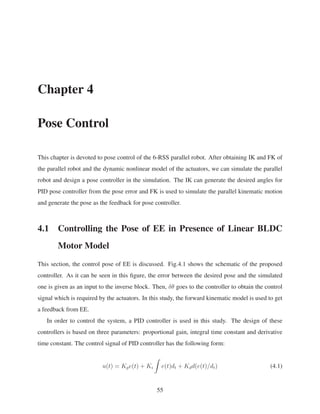
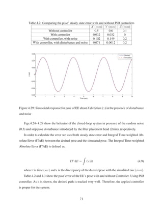
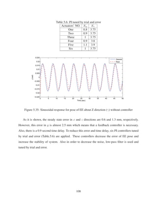
85. Table 4.3: Comparing the pose’ ITAE with and without PID controllers
X (mm.s2
) Y (mm.s2
) Z (mm.s2
)
Without controller 50.2995 47.5572 4.3611
With controller 4.5251 4.6365 0.4032
With controller, with noise 5.9644 5.6992 4.0743
With controller, with disturbance and noise 5.9882 5.9934 3.5813
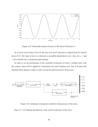
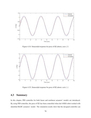
4.2 Controlling the Pose of EE in Presence of Nonlinear BLDC
Motor Model
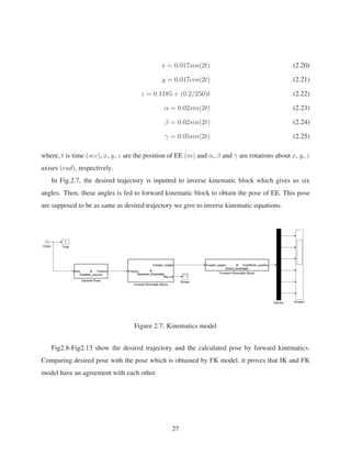
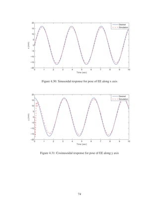
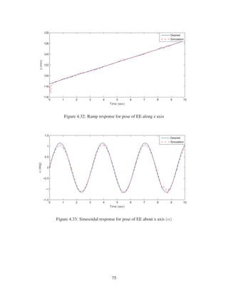
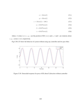
In order to evaluate the performance of the controller, a desired trajectory is defined as follows:
x = 17sin(2t) (4.10)
y = 17cos(2t) (4.11)
z = 118.5 + (0.2/250)t (4.12)
α = 0.02sin(2t) (4.13)
β = 0.02sin(2t) (4.14)
γ = 0.05sin(2t) (4.15)
where, t is time (sec), x, y, z are the position of EE (mm) and α, β and γ are rotations about
x, y, z axises (rad), respectively.
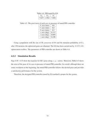
4.2.1 Tuning PID controller Using GA
In this work, GA is used to find the parameters of PID controller. The following objective function
is defined which is the norm of error between the desired pose and actual pose. Using GA, this
objective function should be minimized:
J = ||e||2 (4.16)
where e = [ex, ey, ez, eα, eβ, eγ]T
. For example ex is the error between desired the x position
and actual one. Similarly the other errors can be defined.
72

86. Table 4.4: PID tuned by GA
Kp Kd Ki
7.627 2.561 7.692
Table 4.5: The pose’error of each axis in presence of tuned PID controller
X axis (mm) 0.6
Y axis (mm) 0.4
Z axis (mm) 0.2
α axis (deg) 0.112
β axis (deg) 0.089
γ axis (deg) 0.196
Using a population with the size of 50, crossover of 0.8 and the mutation probability of 0.1,
after 150 iteration, the optimized gains are obtained. The GA has been carried out by MATLAB,
optimization toolbox. The parameters of PID controller are shown in Table 4.4.
4.2.2 Simulation Results
Figs.4.30 - 4.35 show the response for EE’s pose along x, y, z axises. Moreover, Table.4.5 shows
the error of the pose of six axes in presence of tuned PID controller. In overall, although there are
some overshoots at the beginning, the tuned PID controller follows the desired pose and provides
a satisfactory performance for the system.
Therefore, the designed PID controller tuned by GA method is proper for the system.
73

87. 0 1 2 3 4 5 6 7 8 9 10
−20
−15
−10
−5
0
5
10
15
20
Time (sec)
x(mm)
Desired
Simulation
Figure 4.30: Sinusoidal response for pose of EE along x axis
0 1 2 3 4 5 6 7 8 9 10
−20
−15
−10
−5
0
5
10
15
20
Time (sec)
y(mm)
Desired
Simulation
Figure 4.31: Cosinusoidal response for pose of EE along y axis
74

88. 0 1 2 3 4 5 6 7 8 9 10
116
118
120
122
124
126
128
Time (sec)
z(mm)
Desired
Simulation
Figure 4.32: Ramp response for pose of EE along z axis
0 1 2 3 4 5 6 7 8 9 10
−1.5
−1
−0.5
0
0.5
1
1.5
Time (sec)
α(deg)
Desired
Simulation
Figure 4.33: Sinusoidal response for pose of EE about x axis (α)
75

89. 0 1 2 3 4 5 6 7 8 9 10
−1.5
−1
−0.5
0
0.5
1
1.5
Time (sec)
β(deg)
Desired
Simulation
Figure 4.34: Sinusoidal response for pose of EE about y axis (β)
0 1 2 3 4 5 6 7 8 9 10
−3
−2
−1
0
1
2
3
Time (sec)
γ(deg)
Desired
Simulation
Figure 4.35: Sinusoidal response for pose of EE about z axis (γ)
4.3 Summary
In this chapter, PID controller for both linear and nonlinear actuators’ models are introduced.
By using PID controller, the pose of EE has been controlled when the 6-RSS robot worked with
identified BLDC actuators’ model. The simulation results show that the designed controller can
76

90. track different reference signals very well. Also, the robustness of the tuned controller is studied
and it is shown the satisfactory performance of the tuned PID controller in the presence of both
noise and disturbance.
77

91. Chapter 5
Experimental Results
To validate the desired pose control in the real time experiments, we need the accurate measure-
ment of the parallel robot’s pose. Thanks to the newly purchased photogrammetry sensor-C-track
from Creaform Inc. The pose of EE can be measured. The closed-loop feedback pose control
system can be built and the desired pose control can be tested for the pose tracking in real time.
5.1 C-track
In order to validate the kinematics equation C-track has been used. C-track is a system which tracks
the pose of the target. Among many detecting tools, such as laser tracker or vision systems, C-
track can provide accurate measurement at relative low cost. It consists of several part, including;
two cameras which observe the position of robot and send the accurate pose of EE to computer, a
controller, a cone, a calibration bar which used to calibrate the C-track, a handy probe, reflectors
which are called targets.
Figs.5.1 and 5.2 show several parts of C-track.
78

92. (a) Reflector (b) Controller (c) Calibration
Figure 5.1: C-track parts
(d) Handy probe (e) C-track
Figure 5.2: C-track parts
In C-Track, two cameras obtain the positioning targets simultaneously, which enables the soft-
ware to determine the position through triangulation.
Figure 5.3: Capturing targets by two cameras simultaneously
The purpose of this section is to validate the theoretical inverse kinematic model that has been
made in Simulink block. To do so, C-track is used to give the pose of EE. The desired pose is
79

93. given to the inverse kinematic block and applied to the system, and then the robot moves. The pose
of robot is tracked by C-track and the data is sent to VXelements software. Comparing the pose
of EE obtained by C-track with the desired pose input to inverse kinematics, we can validate the
inverse kinematic model.
5.1.1 Hardware Difficulties
In this experimental work we faced with two challenges:
1. Through two computers: Using two quanser cards, the robot is controlled by the computer
(called PC1) and the angle of each actuator could be obtained through Simulink block dia-
gram. Unfortunately the computer that is used for C-track (PC2), differs from the computer
which the parallel robot is connected to. Because C-track needs the high load of computa-
tion, implementing both the C-track data acquisition and control algorithm on one computer
slows down the process and has negative effects on real-time performance of the system.
Also, we have some hardware limitations:
• The C-track license is only used for the PC2.
• The computer that is used for the C-track can not support two Quanser cards.
• The PC2 is also used to control the Fanuc robot which holds the fiber placement head
in the project.
In order to solve the problem, a following experimental setup is built,
80

94. Figure 5.4: Experimental setup for parallel robot
To be able to use the pose measured by C-track for closed-loop controller, the data must be
transferred between two PCs. A Simulink file has been made in which we give the voltage as
an input and get the angles of each actuator as the output of the system. One of the Quanser
card is used to send the applied voltage to six actuators. Each time we run the program,
the power is applied to the actuators and drive both actuators and robot to move. Then, the
potentiometer is used to measure the angle of each actuator. Using the second Quanser card,
the measured data by potentiometer is sent to PC1.
Also, as it is shown, C-track is connected to PC2. The C-track detects the pose of EE and
sends the data to PC2.
2. Using two softwares: The inverse equations code is written in MATLAB, while the cap-
tured data by C-track is sent to VXelements software. In order to form a real-time feedback
system, we need to transfer data from VXelements software to MATLAB or vice versa.
A code is written in Visual Basic (VB) programing language software in which we can connect
81

95. to VXelements software. It means that the data tracked by C-track can be seen, as an output of
the VB code. The goal of using VB is to find a way to transfer the C-track data to MATLAB
software. It is necessary to solve the first mentioned problem. To do so, we use a double serial port
in order to connect two computers. Furthermore, a code is written in VB which exports the data to
serial port and a code is written in MATLAB which imports the data from the serial port.
In order to measure the pose of EE, C-track should be calibrated. The following procedure
illustrates how to calibrate the C-track:
• It should not be placed facing the sun or intense light, because intense light causes an optical
noise in the C-Track field of vision.
• The environment’s temperature should be in the range of was (+/- 2 C) during calibration.
In order to use the handy probe, it should be calibrated as well. To do so, the following se-
quences are followed:
1. We created a dynamic referential prior to calibration.
2. Enough positioning targets were distributed in volume. These targets were not placed sym-
metrically in order to increase the accuracy.
3. We placed the handy probe in the cone which has a distance about 2 m from the C-track. In
order to reduce the error of calibration, the cone should not move during the process. So we
locked the cone to the surface.
4. We clicked on the start bottom to start the calibration and followed the steps shown on the
screen.
82

96. Figure 5.5: Probe calibration
The errors of calibration for both probe and C-track should be less than 0.04 mm. If the process
takes too much time, the accuracy of probing might be influenced.
Firstly, the robot’s EE should be cleaned in order to stick the target on it. The robot should not
be greasy because the target should not move or fall during the measurement. We attached at least
4 targets on the parallel robot where C-track could see these targets. The more targets could be seen
by C-track, the more accurate targets position can be measured. The targets are distributed in the
volume and the positioning target is sticked asymmetrically to increase the accuracy of inspection.
This distribution is affected by many conditions; such as,
• If we spread the targets in longer distances, C-track could measure data in a wider range.
• Covering 3 axis: The target covers 3 axes and gives the C-track adequate reference in all of
these axes.
In this work we tried to consider all above conditions to increase the accuracy.
83

97. Figure 5.6: Parallel robot
In order to work with the software, we need to make a new session first. In our new session,
C-track observed thirteen targets at the same time and these targets are saved as the positioning
targets. As far as C-track could see at least four targets among the positioning targets, we can
work in the VXelements software. C-track has four referencing modes: static, dynamic, sensor
and automatic. Each mode has its own features:
• Sensor mode: In this mode, C-track and part cannot move during the work.
• Dynamic mode: When the environment of work has vibrations, it is suggested to use dy-
namic mode. In this mode the positioning targets need to remain in the place where they are
detected at first time. Each time, a minimum of four positioning targets should be observed
by C-track as well. The most important feature is that we can move the C-track during the
experimental work.
• Static mode: In contrast to dynamic mode, when we use the static mode we are not allowed
84

98. to move the C-track and the part during the measurement. But the advantage of this mode is
C-track does not need to see the targets each time we are measuring.
• Automatic mode: It is a combination of static and dynamic modes. In this kind of mode, a
minimum of one positioning target must to be seen by C-track during the measurement all the
time. If the visible positioning targets are less than four, the system switches to static mode
automatically. Furthermore, the targets could not be obstructed more than five minutes.
In this experimental work, the dynamic referential mode is used because we need to move the
C-tracks location during the measurement.
After creating new session, the first idea was to align a frame as our original (reference) frame
of parallel robot on one of the six motors. Using this method, the pose of EE with respect to the
location of motor (reference frame) could be determined. The main problem was: in the inverse
kinematic equations we used the mid-point of lower platform as an original frame, so in order to
validate the inverse kinematic equations with experimental results, we need to find the pose of EE
with respect to the base frame defined in the inverse kinematics.
Hence, the idea of using actuator’s position as a base frame is changed to find the middle point
of the lower frame of parallel robot. If we attach the target in the middle of base plate, we have
two problems: first the location of mid-point we choose is not accurate enough because it is based
on the observation by eyes. Second, C-track could not see the target on the mid-point. To do so,
we decided to find the mid-point of base frame based on the following sequences:
1. Creating four circles to find point Bi (motor positions):
C-track could not see four motors among six ones at the same time. We were probing several
points on each motors surface. Because we need to create a circle for each motor, we need to
probe at least three points. In VXelements software we chose circle bottom in order to create
the circle. In point selection bottom, we select four points or more on individual circle. The
error of each circle should be less than 0.04 mm. If we select only three points, the software
does give us the error of the created each circle. Then we did the same sequences for every
other wanted circle.
2. Finding the center point of each circle (B1, B2, B3 and B4): After we made four circles, we
85

99. can find the mid-point of each circle. These obtained points are called B1, B2, B3 and B4 in
our inverse kinematic equations, which are the location of four motors (revolute joints).
3. Creating the Circle based on 4 points (B1, B2, B3, B4): After we find the location of each
motor, we click on circle bottom again and choose the point selection. We choose mid-points
of each circle and create our main circle using B1, B2, B3 and B4. If the error is less than
0.04 mm, the created circle is acceptable. If not, we need to repeat our work from Step One.
4. Finding the center of the main circle (O): After creating the main circle, we can obtain the
center point where we want to align the original frame of parallel robot on.
After finding the middle point of the circle, it is time to align the frame, that is according to the
reference frame used in inverse kinematic equations. Aligning the direction of z axis is easy, but
the question is how to align the direction of x axis according to inverse kinematics. In the inverse
kinematic equations, the x-axis is coincidence to the line which passes from referential point to
the middle between B1 and B6 or the x-direction is against of the direction of the line which
passes from referential point to the middle point between B3 and B4 (because robots geometry is
symmetry). Thus, we need to find the mid-point between two motors, and then we can create the
line using the obtained mid-point and reference point. If we want to find the mid-point between
B1 and B6, the problem is that C-track could not see the sixth motor. Accordingly, in order to
solve this problem, we used third and forth motors (B3 and B4) to find the mid-point. Then, we
created the line from reference point to the mentioned mid-point. Using this line, we aligned the
x-direction exactly against the direction of the created line. Using right hand rule for aligning the
frame, we can align the direction of y axis. Now we have our referential frame.
In the next crucial step, we want to align Upper Frame (UP) which shows the pose of EE. In
order to do that, we have done following sequences:
1. Modeling the UP using handy probe: in this step we used handy probe to detect several
points on the surface of UP using optical method. We cannot use touching method, because
in this method, the target should be visible.
Unfortunately, the sticker targets on the surface of the UP are not observed by C-track. So
we used optical probing method. After finding a minimum of three points we created the
plate which is called UP.
86

100. 2. Creating plate A, plate B, plate C, and plate D: using handy probe we probed the points on
the plane A to D, then we created those planes in the VXelements.
Figure 5.7: Parallel robot model in VXelements software
3. Finding the intersection line: The intersection of the two planes is a line. So we find the
intersection line between the plane A and UP (L1), the intersection line between plane B
and UP (L2), the intersection line between plane C and UP (L3), and the intersection line
between plane D and UP (L4).
4. Finding the intersection points: the intersection of two lines is a point. Using four lines
obtained in the previous step we could find the intersection point between two lines. The
intersection point between L1 and L2 is called P1, the intersection point between L2 and L3
is called P2, and the intersection point between L3 and L4 is called P3.
5. Finding the mid-point of both L2 and L3: using P1 and P2, we could find the mid-point of
L2(Pm12 ). Also, we used the P2 and P3 in order to find the mid-point of L3(Pm23 ).
6. Finding the reference point: Based on our knowledge which proves Pm12 is located on the
plane B, we created the new line Lm1 which passed from Pm12 and is normal to plane B.
Also, we knew that Pm23 is located on plane C, so we created the line Lm2 which is normal
87

101. to plane C and passed fromPm23 . Then we intersected these two lines. The intersection point
is the reference point or the EE pose (O ).
Figure 5.8: Finding EE pose
7. Aligning the Upper Frame (O x y z ): In order to align the frame (O x y z ) on the obtained
reference point (O ), we need to create another line which is located in plane D. To do so, we
probed plane F, the same as before, we found the intersection line between UP and plate F
(L5). Using L4 and L5 we found the intersection point (P4). Then, we found the mid-point
between P3 and P4 which is called Pm34 . we created the line from O to the Pm34 . Using this
line, we aligned the x -direction exactly in the direction of the created line. Also, we aligned
the z -direction which is exactly normal to UP. Using right handle rule, the direction of the
y is obtained.
Figure 5.9: Aligning frame O x y z pose
88

102. Now we have both Base Frame and UP, which means that the relationship between the pose
of EE with respect to base frame could be detected by C-track. We fixed the Base Frame as the
original frame, so we can track the pose of parallel robot with respect to the original frame. When
we click on track bottom in the VXelements software, it gives us the pose of EE each 1/29 second.
Then we export this data as a tracking sequence and then importing the tracking sequence in visual
basic (VB) software. There is a written code in VB environment which we can used to see the
results in VB environment. We should make sure that each time we connect the VB software to
C-track in order to see the data, the VXelements software is closed. The reason we should close
the VXelements software is that the C-track cannot connect with two softwares at the same time.
The sequences are shown as follows:
1. Open the code in VXelements.
2. Clicking on “start bottom”, a window shows up.
3. Clicking on “connect to VXelements”.
4. Clicking on open targets, give us the data positioning of original frame.
5. Importing the data (positioning targets) of upper frame and adding this data as a sequence.
6. Completing the previous sequences, the pose of EE with respect to the base frame is shown
in Fig.5.10.
Figure 5.10: Visual basic model
89

103. Table 5.1: Measuring LATi
by C-track
LATi
i = 1 i = 2 i = 3 i = 4 i = 5 i = 6 average
mm 166.861 162.066 165.651 163.263 165.105 159.396 163.7236
Comparing the results tracked by C-track with the desired pose has a huge error which means
the inverse kinematic model is not accurate. All the lengths and angles we used for inverse kine-
matic equations were measured by the ruler, so they were not accurate enough and caused a consid-
erable error. Another reason is due to neglecting the Lz in the initial inverse kinematics to simplify
the equation.
In order to reduce the error, we have calibrated some parameters. The sequences are listed as
follows:
1. Modifying LATi
: At first, we used the value of 165mm for LATi
in the inverse kinematics
equation, which was measured by the ruler. Using the C-track, this value is reduced from
165 mm to 163.7236 mm which is the average of six LATi
. In order to measure the value of
LATi
:
• We probed the sphere Ai (i = 1, 2, 6) and Ti (i = 1, 2, 6).
• Then, we created 6 lines (AT1, AT2, , AT6) and measured the length of line.
• We took the average from line AT1, to line AT6; the final value is 163.7236 mm.
Figure 5.11: Lenght of ATi
90

104. Table 5.2: Measuring Lzi
by C-track
Lzi
i = 1 i = 2 i = 3 i = 4 i = 5 average
mm 40.952 39.836 39.372 38.903 39.016 39.62
2. Adding Lz : first we neglected the Lz, while this length has a value of 39.6158 mm. To
obtain the precise value of Lz :
• Creating four planes: C-track could see only five actuators (B1, B2, B3, B4, B5). So we
created five plates which passed from Bi(i = 1, 2, 5) and paralleled to the base plate.
• Creating four lines: Clicking on point to normal bottom, we created the normal line
from sphere T1to plate B1 and so on (Lz1 , Lz2 , Lz3 and Lz4 ).
• We took the average from line Lz1 , to line Lz5 the final value is 38.455 mm.
Figure 5.12: Lenght of Lz
3. ModifyingLAi
: Using the C-track the values of LA1−2 , LA2−3 LA3−4 , LA4−5 , LA5−6 , LA6−1
have been changed.
91

105. Table 5.3: Measuring LAi
by C-track
LA LA12 LA34 LA56 LA23 LA45 LA61
mm 50.578 51.094 50.629 353.707 354.118 353.823
Average 50.767 353.883
Figure 5.13: Modifying LA
4. Modifying LBT : The initial LBT was considered as 40 mm. This value is measured by the
ruler. To obtain the accurate value of LBT , we have done following steps:
• We created the line which is normal to plate B1 and passed from point B1. This line is
called b1. We created three other lines (b1, b2, b3) like the first one.
• We measured the distance between sphere T1to b1. We measured other three distances.
• We took the average from four distances; the final value is 38.455 mm.
Figure 5.14: Length of BTi
92

106. Table 5.4: Measuring LBTi
by C-track
LBTi
i = 1 i = 2 i = 3 i = 4 average
mm 37.530 39.24 39.230 38.037 38.509
5. Adding the offset to upper frame: The inverse kinematic model considered the EE pose in
the middle of the upper plates thickness, while we considered the EE pose on the surface of
upper plate using C-track. This difference caused 20mm error in z-direction.
In order to reduce the error, we proposed two ways: Changing the inverse kinematics or changing
the model we built. The easiest way is to change the model we have built in the software. So we
created the plate which passed from sphere Ai(i = 1, 2, 6) and is parallel to upper plate. Then we
translated the upper frame to the center of new plate. We gave two sine inputs with the amplitudes
of 10mm in x and y directions, a cosine input with an amplitude of 10 mm in z-direction as three
positions. The following graph compares the results of C-track with desired pose:
Figure 5.15: Sinusoidal response for pose of the EE along X direction
93

107. Figure 5.16: Cosinusoidal response for pose of the EE along Y direction
Figure 5.17: Sinusoidal response for pose of the EE along Z direction
Figs.5.18-5.20 show the errors in X, Y and Z directions are shown. These errors are shown in
Table.5.5 as well.
94

108. Table 5.5: Inverse kinematic validation
Maximum Error in X axis (mm) 0.6
Maximum Error in Y axis (mm) 0.6
Maximum Error in Z axis (mm) 0.4
Figure 5.18: Error X
Figure 5.19: Error Y
95

109. Figure 5.20: Error Z
As you can see, the error in x-direction is changing with respect to time with a sine curvature.
The maximum error is about 0.6 mm. The error in y-direction follows a cosine curvature with
respect to time. The maximum error in y direction is about 0.6 mm while this error in z axis
reaches to 0.4mm. Although, the error of direction seems less than the others ones, the graph
shows too much noise caused by C-track. In overall, although there are still errors in all directions,
the results are satisfactory in practice.
5.2 Transferring Data
This section is devoted to solving communication problem between two computers. In order to
control the pose of EE in real time, the desired pose and the real data must be available at the
same time in one Simulink file so that the signals can be compared with each other for controlling
the robot. As we discussed in previous section, the parallel robot is connected to PC1 and gets
its movement instructions from it. In the same time, PC2 receives the movement data from C-
track. So we need to transfer C-track data from PC2 to PC1. The precise and fast way for this
communication is using serial port (Fig.5.21).
96

110. Figure 5.21: Using serial port for communication
To read the data via C-track, a VB application is written which stores EE pose in six variables
and these variables are updated every 35 miliseconds. The code that specifies parallel robots move-
ment pattern is written in MATLAB. PC1 is chosen as the master computer. As it was discussed
this PC sends movement instructions to robot. To control the robot, it needs the other information
that exists in PC2. So we added a code to the original C-Track code to send the data to PC1. The
protocol that is chosen for data transfer between two computers is serial protocol.
In the first attempt, a MATLAB code was written to receive the information which PC2 was
sending through serial port. The mentioned MATLAB code provided the desired information
in the workspace of MATLAB. Although the written code could show the data in workspace,
Simulink libraries did not support specific elements that were used in that code. So, it is not
possible to use this MATLAB file in Simulink in form of a MATLAB function block. The
solution that we came up with was to use COM1 Module which makes the connection between
two computers possible after it is configured.
Figure 5.22: COM1 block
97

111. Fig.5.22 shows the COM1 Block in Simulink which receives the data from serial port in
MATLAB Simulink and the MATLAB function which is responsible for de-serializing data.
In serial protocol data is sent as ASCII numbers, hence COM1 receives stream of ASCII numbers.
Each ASCII number represents a character as Fig.5.23. By using the Matlab function module code,
the data received from COM1 is transformed from ASCII numbers to real numbers.
Figure 5.23: Stream Client Receiver block
5.2.1 Problem Definition
Using COM1, received data from serial port is sent to MATLAB Simulink. This Simulink only
works in Normal mode because of presence of COM1 module(Fig.5.24)
98

112. Figure 5.24: Normal mode
As it was explained before, two Quanser cards modules are used to make a connection between
the robot and Simulink application. This Simulink only works in External mode (Fig.5.25).
99

113. Figure 5.25: External mode
In order to control the parallel robot we need to have desired pose and C-track pose in one
Simulink block diagram. It is not possible to run one MATLAB Simulink block diagram in two
different modes (Normal and External) at the same time.
100

114. Figure 5.26: Normal and external modes
Fig.5.26 shows the Simulink block diagram which is proposed in order to see the C-track data
and desired pose simultaneously. We must solve the problem which is to operate the robot while
the serial port is only working in Normal mode.
5.2.2 Solution
Stream Client and Stream Server are the modules which work in both normal and external. Their
purpose is to send and receive data by using specified protocol. To solve the problem two following
steps were taken:
1. Opening two Matlab files simultaneously: Two Matlab Simulink block diagrams in two
different Matlab compilers are opened. One of them works in normal mode (Simulink1) which
receives the data from serial port. The other one works in External mode (Simulink2) which is
connected to parallel robot.
2. Using Stream Client and Stream Blocks: In order to send the data from Normal mode to
External mode, Stream Client blocks are used. While Simulink1 is running, the data can be sent
through Stream Server to Simulink2 which receives the data by using Stream Client block.
101

115. Figure 5.27: Stream Client Sender block
In Fig.5.27, COM1 receives the data from PC2 continuously. Since the serial port transfers all
data together, a MATLAB function is written to separate the pose data from each other. Also,
COM1 receives all data as ASCII numbers. So, a code is written in which the groups of ASCII
numbers are transformed into real numbers. In these codes, the serial receiver module receives
77 ASCII characters in each transaction. Each parameter (x, y, z, α, β and γ) is made of ten
characters. After each set of ten characters, there is one newline character which means that a new
parameter is started. The remaining 11 characters are ten zeros and one new line which specifies
the start of each set of received data. After finding ten zeros and the newline character parameters
x, y, z, α, β and γ are retrieved.
Fig.5.28 shows Simulink2 which receives all data from Simulink1. As a result, both C-track
data and desired pose are available in one Simulink application and the feedback controller can be
built to reduce the error between desired pose and C-track pose in real time.
102

116. Figure 5.28: Stream Client Receiver block
5.3 Control the Pose of EE
In order to control the pose of end-effector, in the previous section, all the data which were obtained
by C-track are transferred from PC2 to PC1. Then, two Matlab files were opened and two Simulink
files were running simultaneously. Using the stream client block, all data were transferred from one
Simulink file that worked in normal mode to another Simulink file that worked in external mode.
In this section, the data transferred is used to control the pose of EE. As it is shown in Fig.5.29, a
Simulink block diagram is built in which the desired pose is input to the inverse kinematic block
to generate the desired angles for the actuators. Six Stream Client blocks give the pose of EE.
Then actuators’ angles are compared with real actuators’ angles from experiment and six errors
are given to PI controllers. PI controllers minimized the error. By using trial and error, different
kI terms and kP terms are obtained for six PI controllers. Unfortunately, PID controller could not
103

117. be used for the system. Because each time kd was added to the controller, the feedback system
became unstable in experiment and it might ruin the actuators. Also, six different low pass filters
are used to reduce the noise of system.
Figure 5.29: PID controller
In order to evaluate the performance of controller, a different desired trajectory is defined as
follows:
104

118. x = 10sin(t) (5.1)
y = 10cos(t) (5.2)
z = 10sin(t) + 198.5 (5.3)
α = 0.0175sin(t) (5.4)
β = 0.0175sin(t) (5.5)
γ = 0.0175sin(t) (5.6)
where, t is time (sec), x, y, z are the position of EE (mm) and α, β and γ are rotations about
x, y, z axises (rad), respectively.
Fig.5.30-5.35 show the behavior of system without using any controller and low pass filter.
0 5 10 15 20 25 30
−10
−5
0
5
10
Time (sec)
Y(mm)
Desired
Real
Figure 5.30: Sinusoidal response for pose of EE about X direction without controller
105

119. Figure 5.31: Cosinusoidal response for pose of EE along Y direction without controller
Figure 5.32: Sinusoidal response for pose of EE along Z direction without controller
106

120. Figure 5.33: Sinusoidal response for pose of EE about X direction (α) without controller
Figure 5.34: Sinusoidal response for pose of EE about Y direction (β) without controller
107

121. Table 5.6: PI tuned by trial and error
Actuators’ NO. Kp Ki
One 0.8 3.75
Two 0.9 3.75
Three 1 3.75
Four 0.9 3.8
Five 1.1 3.9
Six 1 3.75
Figure 5.35: Sinusoidal response for pose of EE about Z direction (γ) without controller
As it is shown, the steady state error in x and z directions are 0.6 and 1.3 mm, respectively.
However, this error in y is almost 2.5 mm which means that a feedback controller is necessary.
Also, there is a 0.9 second time delay. To reduce this error and time delay, six PI controllers tuned
by trial and error (Table.5.6) are applied. These controllers decrease the error of EE pose and
increase the stability of system. Also in order to decrease the noise, low-pass filter is used and
tuned by trial and error.
108

122. Figure 5.36: Sinusoidal response for pose of EE along X direction, using PI controller
Figure 5.37: Cosinusoidal response for pose of EE along Y direction, using PI controller
109

123. Figure 5.38: Sinusoidal response for pose of EE along Z direction, using PI controller
Figure 5.39: Sinusoidal response for pose of EE about X direction (α), using PI controller
110

124. Figure 5.40: Sinusoidal response for pose of EE about Y direction (β), using PI controller
Figure 5.41: Sinusoidal response for pose of EE about Z direction (γ), using PI controller
Figs.5.36-5.41 show the behavior of system in presence of PI controller. As it is shown, tuning
six different PI controllers, decreased the average of time delay from 0.9 to almost 0.3 sec. While
the error of z does not have a significant change (from 1.3 to 1.1mm), the error in y direction has
reduced 10 times, from 2.5 to 0.25 mm. It is not possible to use Kd, because it makes real system
unstable. As a result, system has some overshoots in each direction. In Table.5.7, the steady state
error of system with a controller is compared with a non-controller system in each direction. Also,
Table.5.8 shows the Integral Time-weighted Absolute Error (ITAE) of the system with and without
111

125. Table 5.7: Comparing the pose’ steady state error with and without PI controllers
Without controller With controller
X axis (mm) 0.7 0.75
Y axis (mm) 2.5 0.25
Z axis (mm) 1.3 1.1
α (rad) axis 0.0055 0.004
β axis (rad) 0.0015 0.00145
γ axis (rad) 0.0025 0.002
Table 5.8: Comparing the pose’ITAE with and without PI controllers
Without controller (mm.s2
) With controller (mm.s2
)
X axis (mm) 2669 2055.9
Y axis (mm) 2971.9 2390.7
Z axis (mm) 2824.4 2198.7
α (rad) axis 6.0267 5.2366
β axis (rad) 5.0559 4.5198
γ axis (rad) 5.3485 4.6625
the controller.
Although increasing kI for each controller add some overshoots at the beginning of each graph,
steady state error decreased significantly which means that applied PI controller is robust and has
an acceptable pose tracking control.
5.4 Comparing the Simulation and Experimental Results
In order to compare the simulation results of pose control of EE with the experimental ones, we
used normalized time instead of real time to calculate the Integral Time-weighted Absolute Error
(ITAE) as follow,
ITAE = ¯t| |d¯t (5.7)
where ¯t = t/T is normalized time, T is total time, and is the error between the desired pose
with the calculated pose (mm).
Table.5.9 compares the errors obtained from simulations with the errors from experiments
(Table.5.10 ).
112

126. Table 5.9: Normalized ITAE of the EE’s pose in simulations
X (mm) Y (mm) Z (mm)
Without controller 0.5030 0.476 0.0436
With controller 0.0453 0.0464 0.0040
With controller, with noise 0.0596 0.0570 0.0407
With controller, with disturbance and noise 0.0599 0.0599 0.0358
Table 5.10: Normalized ITAE of the EE’s pose in experiments
Without controller (mm) With controller (mm)
X axis (mm) 1.0676 0.8244
Y axis (mm) 1.1888 0.9563
Z axis (mm) 1.1298 0.8795
α (rad) axis 0.0024 0.0021
β axis (rad) 0.0020 0.0018
γ axis (rad) 0.0021 0.0019
As it is shown, the error of pose in simulations is less than that of experiments. There are
several reasons that cause to have more error in experimental works, such as:
• There are always some uncertainties which cause some errors between the real parameters
and measured ones, such as the length of links.
• Transferring the data between two computers causes time delay.
• We cannot use Kd gain for design the PI controller in experiments, because it caused to
system become unstable.
• Like every other sensors, C-track cause the noise.
5.5 Summary
This chapter has described the experimental setup including the C-track, communication between
two computers, 6-DOF Robot and controller, and also results for proposed PI controllers. In this
chapter C-track is implemented to obtain the pose of EE. While the robot is connected to PC1, the
achieved pose by C-track stores in PC2. Data has been transfered from PC2 to PC1 by using serial
port. Two Simulink block diagrams are made to receives the data from serial port and move the
robot simultaneously. In order to control the pose of EE, 6 different PI controllers is applied and
113

127. increase the robustness of the system. The results with and without the presence of controllers are
compared and discussed.
114

128. Chapter 6
Conclusion
This chapter summarize the main conclusions and contributions of previous chapters. Meanwhile,
some future works are presented.
6.1 Contribution and Research Conclusion
In order to obtain more dexterity to produce complex composite structures, a 6-RSS parallel robot
is added to current Automated Fiber Placement (AFP) machines. The present research study is de-
voted to modeling and control of 6 RSS parallel platform. The main contributions and conclusions
of this research work is listed as follows:
• The inverse and forward kinematics of 6-RSS parallel robot are analyzed.
• The dynamic models (linear and nonlinear) for parallel’s actuators have been built. The
parameters of linear dynamic models have been identified using Genetic Algorithm (GA).
Also, the multi-objective optimization using GA was applied to find the parameters of the
nonlinear DC actuators’ dynamic model of the 6-RSS parallel robot in the lab.
• A PID controller is designed and optimized using GA to control the EEs pose of the 6-
RSS parallel robot. The simulation results indicated that the optimized PID controller has a
satisfactory pose tracking performance.
• A C-track was applied to obtain the precise values for position and orientation of EE.
115

129. • Then, inverse kinamtic model has been validated in experiment. Comparing the desired
pose with the obtained pose by C-track proved that the inverse kinematic model is accurate
enough.
• In the experimental work, two different PCs are used. One of them stored the obtained pose
by C-track. The other one, moved the parallel robot. By transferring the data from First PC
to second one and running two Simulink models at the same time, we are able to control the
pose of EE and made it possible to have the feedback from pose of the system.
• Finally, six different PI controllers have been implemented to the robot to determine the
control input for the six actuators. Using these control inputs, the pose of EE has been
controlled. Experimental results showed the satisfactory pose tracking control performance.
6.2 Future Works
The future works of this thesis include the following:
• The model based controllers such as feedback linearizion will be implemented in the exper-
imental setup which includes the pose measurement using C-track.
• The designed PI controllers will be fine tuned by using multi-objective optimization tech-
nique to deliver better tracking performance.
• The real-time pose controller will be integrated with the Fanuc robot to realize the coopera-
tive fiber placement operation.
116

130. Bibliography
[1] Dan Zhang. Parallel robotic machine tools. Springer Science & Business Media, 2009.
[2] Doug Stewart. A platform with six degrees of freedom. Proceedings of the institution of
mechanical engineers, 180(1):371–386, 1965.
[3] Shuang Cong, Guodong Li, and Xianyong Feng. Parameters identification of nonlinear dc
motor model using compound evolution algorithms. In Proceedings of the World Congress
on Engineering, volume 1, 2010.
[4] Feng Gao, Weimin Li, Xianchao Zhao, Zhenlin Jin, and Hui Zhao. New kinematic struc-
tures for 2-, 3-, 4-, and 5-dof parallel manipulator designs. Mechanism and machine theory,
37(11):1395–1411, 2002.
[5] Serdar Kucuk and Zafer Bingul. Robot kinematics: forward and inverse kinematics. INTECH
Open Access Publisher, 2006.
[6] X Shi and RG Fenton. Solution to the forward instantaneous kinematics for a general 6-dof
stewart platform. Mechanism and machine theory, 27(3):251–259, 1992.
[7] Meng-Shiun Tsai, Ting-Nung Shiau, Yi-Jeng Tsai, and Tsann-Huei Chang. Direct kinematic
analysis of a 3-prs parallel mechanism. Mechanism and Machine Theory, 38(1):71–83, 2003.
[8] Xiguang Huang, Qizheng Liao, Shimin Wei, Xu Qiang, and Shuguang Huang. Forward kine-
matics of the 6-6 stewart platform with planar base and platform using algebraic elimination.
In Automation and Logistics, 2007 IEEE International Conference on, pages 2655–2659.
IEEE, 2007.
117

131. [9] Zheng Geng and L Haynes. Neural network solution for the forward kinematics problem of a
stewart platform. In Robotics and Automation, 1991. Proceedings., 1991 IEEE International
Conference on, pages 2650–2655. IEEE, 1991.
[10] Kevin Cleary and Thurston Brooks. Kinematic analysis of a novel 6-dof parallel manipulator.
In Robotics and Automation, 1993. Proceedings., 1993 IEEE International Conference on,
pages 708–713. IEEE, 1993.
[11] Kai Liu, John M Fitzgerald, and Frank L Lewis. Kinematic analysis of a stewart platform
manipulator. Industrial Electronics, IEEE Transactions on, 40(2):282–293, 1993.
[12] PR McAree and RW Daniel. A fast, robust solution to the stewart platform forward kinemat-
ics. Journal of robotic systems, 13(7):407–427, 1996.
[13] Yunfeng Wang. An incremental method for forward kinematics of parallel manipulators. In
Robotics, Automation and Mechatronics, 2006 IEEE Conference on, pages 1–5. IEEE, 2006.
[14] Choon seng Yee and Kah-bin Lim. Forward kinematics solution of stewart platform using
neural networks. Neurocomputing, 16(4):333–349, 1997.
[15] Zongliang Mu and Kazem Kazerounian. A real parameter continuation method for complete
solution of forward position analysis of the general stewart. Journal of Mechanical Design,
124(2):236–244, 2002.
[16] Pratik J Parikh and Sarah S Lam. Solving the forward kinematics problem in parallel ma-
nipulators using an iterative artificial neural network strategy. The International Journal of
Advanced Manufacturing Technology, 40(5-6):595–606, 2009.
[17] Antonio Morell, Mahmoud Tarokh, and Leopoldo Acosta. Solving the forward kinemat-
ics problem in parallel robots using support vector regression. Engineering Applications of
Artificial Intelligence, 26(7):1698–1706, 2013.
[18] CM Liaw, RY Shue, HC Chen, and SC Chen. Development of a linear brushless dc motor
drive with robust position control. In Electric Power Applications, IEE Proceedings-, volume
148, pages 111–118. IET, 2001.
118

132. [19] Rolf Isermann and Marco M¨unchhof. Application examples. Identification of Dynamic Sys-
tems, pages 605–682, 2011.
[20] Tolgay Kara and Ilyas Eker. Nonlinear modeling and identification of a dc motor for
bidirectional operation with real time experiments. Energy Conversion and Management,
45(7):1087–1106, 2004.
[21] Radojka Krneta, Sanja Anti´c, and Danilo Stojanovi´c. Recursive least squares method in
parameters identification of dc motors models. Facta universitatis-series: Electronics and
Energetics, 18(3):467–478, 2005.
[22] Mehdi Nasri, Hossein Nezamabadi-Pour, and Malihe Maghfoori. A pso-based optimum de-
sign of pid controller for a linear brushless dc motor. World Academy of Science, Engineering
and Technology, 26(40):211–215, 2007.
[23] G Mamani, J Becedas, V Feliu-Batlle, and H Sira-Ramirez. Open-loop algebraic identifica-
tion method for a dc motor. In Control Conference (ECC), 2007 European, pages 3430–3436.
IEEE, 2007.
[24] Jinzhu Peng and Rickey Dubay. Identification and adaptive neural network control of a dc
motor system with dead-zone characteristics. ISA transactions, 50(4):588–598, 2011.
[25] Bharat Bhushan and Madhusudan Singh. Adaptive control of dc motor using bacterial forag-
ing algorithm. Applied Soft Computing, 11(8):4913–4920, 2011.
[26] Wei Wu. Dc motor parameter identification using speed step responses. Modelling and
Simulation in Engineering, 2012:30, 2012.
[27] Amro M Farid and S Masoud Barakati. Dc motor neuro-fuzzy controller using pso identifica-
tion. In Electrical Engineering (ICEE), 2014 22nd Iranian Conference on, pages 1162–1167.
IEEE, 2014.
[28] Chin-I Huang, Chih-Fu Chang, Ming-Yi Yu, and Li-Chen Fu. Sliding-mode tracking control
of the stewart platform. In Control Conference, 2004. 5th Asian, volume 1, pages 562–569.
IEEE, 2004.
119

133. [29] Chin-I Huang and Li-Chen Fu. Smooth sliding mode tracking control of the stewart platform.
In Control Applications, 2005. CCA 2005. Proceedings of 2005 IEEE Conference on, pages
43–48. IEEE, 2005.
[30] Dong Sun, R Lu, James K Mills, and C Wang. Synchronous tracking control of parallel ma-
nipulators using cross-coupling approach. The International Journal of Robotics Research,
25(11):1137–1147, 2006.
[31] Xiaocong Zhu, Guoliang Tao, Bin Yao, and Jian Cao. Adaptive robust posture control of par-
allel manipulator driven by pneumatic muscles with redundancy. Mechatronics, IEEE/ASME
Transactions on, 13(4):441–450, 2008.
[32] Dongya Zhao, Shaoyuan Li, and Feng Gao. Fully adaptive feedforward feedback synchro-
nized tracking control for stewart platform systems. International Journal of Control, Au-
tomation, and Systems, 6(5):689–701, 2008.
[33] Yang Bo, Pei Zhongcai, and Tang Zhiyong. Fuzzy pid control of stewart platform. In Fluid
Power and Mechatronics (FPM), 2011 International Conference on, pages 763–768. IEEE,
2011.
[34] Xue Jian, Tang Zhiyong, and Pei Zhongcai. Study on stewart platform control method based
on model reference adaptive control. In Cyber Technology in Automation, Control, and Intel-
ligent Systems (CYBER), 2011 IEEE International Conference on, pages 17–20. IEEE, 2011.
[35] S Srikanth and G Ramesh Chandra. Modeling and pid control of the brushless dc motor
with the help of genetic algorithm. In Advances in Engineering, Science and Management
(ICAESM), 2012 International Conference on, pages 639–644. IEEE, 2012.
[36] Sahar Alinia, Masoud Hemmatian, Wen Fang Xie, and Rui Zeng. Posture control of 3-dof
parallel manipulator using feedback linearization and model reference adaptive control. In
Electrical and Computer Engineering (CCECE), 2015 IEEE 28th Canadian Conference on,
pages 1145–1150. IEEE, 2015.
[37] Lorenzo Sciavicco and Bruno Siciliano. Modelling and control of robot manipulators.
Springer Science & Business Media, 2012.
120

134. [38] W.L.G.Pollard JR. Spray painting machine, August 27 1940. US Patent 2,213,108.
[39] Pollard Willard LV. Position-controlling apparatus, June 16 1942. US Patent 2,286,571.
[40] Oscar Reinoso, Rafael Aracil, and Roque Saltar´en. Using Parallel Platforms as Climbing
Robots. INTECH Open Access Publisher, 2006.
[41] Bashar S El-Khasawneh and Placid M Ferreira. Computation of stiffness and stiffness bounds
for parallel link manipulators. International Journal of Machine Tools and Manufacture,
39(2):321–342, 1999.
[42] Vincent Nabat, Rodriguez de la O, O Mar´ıa, Olivier Company, S´ebastien Krut, and Franc¸ois
Pierrot. Par4: very high speed parallel robot for pick-and-place. In Intelligent Robots and
Systems, 2005.(IROS 2005). 2005 IEEE/RSJ International Conference on, pages 553–558.
IEEE, 2005.
[43] J¨urgen Hesselbach, Jan Wrege, Annika Raatz, and Oliver Becker. Aspects on design of high
precision parallel robots. Assembly Automation, 24(1):49–57, 2004.
[44] Tzung-Cheng Tsai and Yeh-Liang Hsu. Development of a parallel surgical robot with auto-
matic bone drilling carriage for stereotactic neurosurgery. Biomedical Engineering: Applica-
tions, Basis and Communications, 19(04):269–277, 2007.
[45] Zhenhua Wang, Liguo Chen, and Lining Sun. An integrated parallel micromanipulator with
flexure hinges for optical fiber alignment. In Mechatronics and Automation, 2007. ICMA
2007. International Conference on, pages 2530–2534. IEEE, 2007.
[46] Rui Zeng, Shuling Dai, Wenfang Xie, and Bhat Rama. Constraint conditions determination
for singularity-free workspace of central symmetric parallel robots. IFAC-PapersOnLine,
48(3):1930–1935, 2015.
[47] Gwo-Ruey Yu and Rey-Chue Hwang. Optimal pid speed control of brush less dc motors
using lqr approach. In Systems, Man and Cybernetics, 2004 IEEE International Conference
on, volume 1, pages 473–478. IEEE, 2004.
[48] Sidney A Davis. Brushless dc motor, January 18 1977. US Patent 4,004,202.
121

135. [49] Thomas J Sokira and Wolfgang Jaffe. Brushless dc motors: electronics commutation and
controls. Tab Books, 1990.
[50] Atef Saleh Othman Al-Mashakbeh. Proportional integral and derivative control of brushless
dc motor. European Journal of Scientific Research, 35(2):198–203, 2009.
[51] Thomas M Jahns. Motion control with permanent-magnet ac machines. Proceedings of the
IEEE, 82(8):1241–1252, 1994.
[52] Gui-Jia Su and John W McKeever. Low-cost sensorless control of brushless dc motors with
improved speed range. Power Electronics, IEEE Transactions on, 19(2):296–302, 2004.
[53] Siri Weerasooriya and MA El-Sharkawi. Identification and control of a dc motor using
back-propagation neural networks. Energy Conversion, IEEE Transactions on, 6(4):663–
669, 1991.
[54] S Singer and J Appelbaum. Starting characteristics of direct current motors powered by solar
cells. Energy Conversion, IEEE Transactions on, 8(1):47–53, 1993.
[55] NA Rahim, MN Taib, and MI Yusof. Nonlinear system identification for a dc motor using
narmax approach. In Sensors, 2003. AsiaSense 2003. Asian Conference on, pages 305–311.
IEEE, 2003.
[56] Amir Hajiloo and Wen-Fang Xie. Multi-objective optimal fuzzy fractional-order pid con-
troller design. Journal ref: Journal of Advanced Computational Intelligence and Intelligent
Informatics, 18(3):262–270, 2014.
[57] SN Sivanandam, Sai Sumathi, SN Deepa, et al. Introduction to fuzzy logic using MATLAB,
volume 1. Springer, 2007.
[58] Melanie Mitchell. An introduction to genetic algorithms. MIT press, 1998.
[59] Zhixin Yang, Wui Ian Hoi, and Jianhua Zhong. Gearbox fault diagnosis based on artificial
neural network and genetic algorithms. In System Science and Engineering (ICSSE), 2011
International Conference on, pages 37–42. IEEE, 2011.
122

136. [60] Darrell Whitley. A genetic algorithm tutorial. Statistics and computing, 4(2):65–85, 1994.
[61] Dymytro Skybyk. Polyphase brushless dc and ac synchronous machines, August 2 1994. US
Patent 5,334,898.
[62] Shi-Zhong He, Shaohua Tan, Feng-Lan Xu, and Pei-Zhuang Wang. Fuzzy self-tuning of pid
controllers. Fuzzy sets and systems, 56(1):37–46, 1993.
[63] Allan B Plunkett. Field orientation control of a permanent magnet motor, March 21 1989.
US Patent 4,814,677.
[64] Kouhei Ohnishi, Masaaki Shibata, and Toshiyuki Murakami. Motion control for advanced
mechatronics. Mechatronics, IEEE/ASME Transactions on, 1(1):56–67, 1996.
123