This document analyzes the motion of a two-link robotic arm manipulator using MATLAB. It develops linearized equations of motion and proportional controllers for each joint to simulate the robot's movement from an initial to final position. Graphs are generated to compare the desired and actual motion paths, velocities, accelerations, and positions over time. The results show larger errors in the actual path as the end effector moves farther from the linearized region around the initial position. Replacing the proportional controller with a PID controller is suggested to improve precision.

1. Two Link Robot Analysis
May 4, 2016
By
Travis Heidrich

2. Abstract
The two link robotic arm manipulator analyzed in this report is required to be accurate and achieve great precision when
moving from the home position (position 1) to reachable positions within the workspace. The applications of two link
robots are continuously developing. For example they are utilized in the medical field and manufacturing which are
very different industries. In this study the two link manipulator was analyzed to develop the relationship between the
ideal motion as it relates to the actual motion of the joints and end effector in the xy plane. Linearized equations of
motion (EOM) were used to develop proportional controllers for each joint. The full EOM are used to simulate the
manipulator as it moves in the xy plane. Using the coefficients of the cubic polynomial that moves the manipulator from
position 1 to position 2, plots were generated to visualize the changes in the robot’s position, velocity and acceleration
over 0.5 seconds. The polynomials of the two-segment continuous-acceleration trajectory were found and used to
compare the desired x versus y path to the actual x versus y path. It was found that the error occurred when the end
effector reached position 2 which was outside of the linearized region around position 1. The inertial and mass effects
significantly influenced the end effectors precision. It is observed that the end effector’s error is large as it moves from
position 3 to the via point and increase to the position once the end effector reaches its stopping position 5 it entirely
missed the desired location.
Purpose
This two link robotic arm study is intended to analyze
the relationship between the desired and actual motion
and path taken by the robot during operation. Using the
linearized EOM and the coefficients of the cubic
polynomial, the simulation of the manipulator to move
from position 1 to position 2. The polynomials for the
two-segment continuous-acceleration trajectory of the
manipulator can be used to analyze the comparison
between the desired and actual x versus y path. The
analysis in this study creates a visualization of the
robot’s physical constraints and how they affect its
operation. One can employ this analysis to understand
when and why error associated with the manipulator
occurs during the robot’s operation.
Approach
Using the MATLAB program a code was written to
analyze the robot’s motion in the xy plane and changes
in the angular velocity and acceleration of both joints
and the end effector. The MATLAB code is designed to
develop the various graphs that follow to simulate the
location on both joints and end effector with respect to
time and determine the true effects of the robot’s
physical constraints as they relate to the actual motion
versus the ideal motion of the robot. The transformation
matrices are designed to capture the relationship
between the reference frames of the links of the robot.
The associated kinematic equations of the robot are used
to determine the joint parameters that provide a desired
position for the end effector. The positions of motion,
constant variables, gains of each joint’s proportional
controller and transfer functions are defined prior to the
development of the linear and nonlinear EOM. The
respective plots which follow are developed to illustrate
how the two link robot moves in 2D space and what
region in its workspace does it encounter error
associated with the end effector not reaching the desired
end position. Some plots are developed to identify
causes of error related to the robot’s operation and
physical constraints.
Results
The two-link manipulator shown is motionless at the
home position P1 = (θ1=15o
, θ2=135o
).
-
The objective of this project is to model a two link
robot using MATLAB.
 Use linearized EOM for the manipulator and
develop proportional controllers for each
joint. Use position 1 (θ1 = 15o
, θ2 = 135o)
 Using EOM to simulate the manipulator as it
moves from rest to position two.
 Determine the coefficients of the cubic
polynomial that move the manipulator from
rest at position one to position 2 in 0.5 sec.

3.  Find the two-segment continuous-
acceleration trajectory desired polynomials
for the motion from position 3 through a “via
point” at position 4 to the final position 5.
Parts 1 & 2: Plot θ1 vs Time and θ2 vs Time
Graph 1 below plots θ1 and θ1 versus time. The desired
plot was developed using the link parameters and
proportional controller’s joint constraints of ωn = 3 Hz
and ζ = 0.707. The angles provided can be seen in
Graph 3. When developing this graph, proportional
controllers were utilized for each joint together with the
full equation of motion (EOM).
Graph 1: Simulated Thetas vs Time
Part 3: Plot X vs Y Path
The previous graph is useful to see how the angles
respond over time. To observe how the robot moves in
space, it is necessary to look at graph 2 that plots the X
versus Y position of the end effector as it moves from
rest at position 1 to the destination at position 2. When
comparing (actual motion) graph 2 with (desired
motion) graph 6 it is observed that they don’t follow the
same path. Their stopping position is roughly at the
same. They don’t have the same path because of the
physical constraints of the robot’s links. This is due to
the fact that the robot’s links have inertia and mass that
needs to be taken into account. The end position error is
a result of the fact the proportional controller is designed
to work in the linearized region around position 1. The
error will increase the farther the end position is from
that area at position 1. Position 2 is close enough to
position 1 that the error is very small, but larger errors
are expected at larger extensions of the arm.
Graph 2: Trace of X vs Y Path
Part 4: Plot Desired Position vs Time
Graph 3 below shows the desired position versus time
in joint space. After finding the coefficients of the cubic
polynomial that moves the manipulator from rest at
position 1 to position 2 (θ1 = 90o
θ2 = 10o
) change in both
angles was plotted with respect to time. It creates a
visualization of a smooth continuous curve. This was
generated using positions 1 and 2 with the cubic
polynomial and a time of 0.5 seconds.
Graph 3: Desired Angles of Theta vs. Time
Part 5: Plot Angular Velocity vs Time
Graph 4 below demonstrates the desired angular
velocity versus time for the two joints. These joints are
moving from position 1 to position 2 (θ1 = 90o
θ2 = 10o
)
in 0.5 sec. The coefficients of the cubic polynomial

4. were found to create the visualization of how the
angular velocities of both joints change over time.
Graph 4: Desired Velocities of Thetas versus Time
Part 6: Plot Desired Acceleration vs Time
Graph 5 below shows the desired acceleration versus
time for the robot in joint space. The straight line
suggests a constant jerk on both joints. It is a derivative
of the velocity curve that was developed with taking the
derivative of the velocity equation.
Graph 5: Desired Acceleration of Thetas vs. Time
The desired x y path is shown in Graph 6 below. This is
the desired path generated from the cubic polynomial
displayed in Cartesian space.
Graph 6: Desired Path Trace
Graph 7 below is a visualization of what motion the
robot actually performed when moving from position 1
to position 2 (θ1 = 90o
θ2 = 10o
). Graph 7 takes into
account the errors in the controls.
Graph 7: Simulated Trace of Path
Part 7: Plot Desired Position vs Time
Graph 8 below shows in Cartesian space the desired
position vs time of x and y of the manipulator from
position 1 to position 2 over a time of 0.5 sec.

5. Graph 8: Position Y vs Time and Position X vs Time
Graph 9 below shows the step response. The lines that
represent theory (green and purple) would be the
electrical impulses that drive the robot’s motors. Due to
losses, gravity and errors the electrical impulses needed
are larger than the theory. The blue and red lines on the
step response graph represent the electrical impulse
applied. They are intended to create a visualization of
the actual movement of the robot in MATLAB.
Graph 9: Step Responses
Part 8: Plot the Desired X vs Y and the Actual X vs
Y Moving from Position 3 - Position 4 – Position 5
Graph 10 below demonstrates the desired X vs Y path
of the robot’s end effector. The curves are smooth and
efficient with some arcs connecting the start position,
via point and stop position.
Graph 10: Desired XY Path Trace (P3-P5)
Graph 11 below demonstrates the actual path of the
robot in the xy plane of the robot’s end effector. The
error deviation from the desired path starts out rather
large as the end effector moves from position 3 (θ1 =
90o
, θ2 = 45o) in the lead up to the “via point” to position
4 (θ1 = 60o
, θ2 = 60o). As the end effector moves farther
away from the via point the error increases. Once the
end effector reaches position 5 (θ1 = 30o
, θ2 = 20o) the
error is so large that the robot misses the final position
that is desired.
Graph 11: Simulated XY Path Trace (P3-P5)

6. Future Work
The proportional controller should be replaced by a
proportional-integral-derivative (PID) controller. This
type of a controller is a control loop feedback controller.
They are designed to continuously calculate an error
value as the difference between a desired set point and
the process variable measured. The PID controller over
time works to minimize the error by adjusting the
control variable.
Conclusion
Comparing graph 2 (actual motion) to graph 6 (desired
motion) the two link robot’s path is not equivalent. The
ending position is roughly the same, but the path they
follow is not because the robots links have inertia and
mass that should be considered. Although, those
physical characteristics are not know. There is
significant end position error because the proportional
controller is designed to work in the linearized region
around position 1 (θ1 = 15o
θ2 = 135o
). The error is
expected to increase the farther the end position is
laterally from the area at position 1. The inertial and
mass effects do not influence the error as severe because
the distance from position 1 to position 2 is only 20 cm.
The absolute value of angular velocity and angular
acceleration for joint 2 was larger than that of joint 1.
When considering the error associated with the controls
it is clear that graph 7 (actual path) demonstrates how
the robot’s path differs from graph 6 (desired path).
Graph 8 demonstrates the need for a larger input of
electrical impulses than the theoretical requirements to
meet the power requirement. Finally, graph 10 and 11
simulate the path taken by the robot from position 3 (θ1
= 90o
, θ2 = 45o
) through the “via point” position 4 (θ1 =
60o
, θ2 = 60o
) and stopping at position 5 (θ1 = 30o
, θ2 =
20o
). When designing a two link robot the physical
constraints associated with the motors and the inertia
and mass of the components must be considered to
ensure optimal precision of the robot’s end effector. A
major design consideration when selecting motors for
the robot is determining the linearization constraints
associated with different motors. As seen in this study
there were significant errors associated with the
proportional controller because it is designed to operate
in the linearized region around position 1.

7. Two Link Robot MATLAB Code
%% Travis John Heidrich
%% Two Link Robot Analysis
%% May 1, 2016
%% Clean Up
clear all
close all
clc
%% Define Parameters
% Define Robot Dimensions
Izz1 = 0; %N*m*s^2
Izz2 = 0; %N*m*s^2
% this is the motor armature inertia, already reflected thru the gear ratio
M1 = 0.035; % kg
M2 = 0.067; % kg
L1 = 0.2; % m
L2 = 0.3; % m
% Create Transforms
syms ai alphai di thetai theta1temp theta2temp
Tx=[1 0 0 0;0 cos(alphai) -sin(alphai) 0;0 sin(alphai) cos(alphai) 0;0 0 0 1];
Dx=[1 0 0 ai;0 1 0 0;0 0 1 0;0 0 0 1];
Tz=[cos(thetai) -sin(thetai) 0 0;sin(thetai) cos(thetai) 0 0;0 0 1 0 ;0 0 0 1];
Dz=[1 0 0 0;0 1 0 0;0 0 1 di;0 0 0 1];
%Concatenate in one homogeneous transform
AtB=Tx*Dx*Tz*Dz;
ai = 0;
alphai = 0;
thetai = theta1temp;
di = 0;
T01 = subs(AtB);
ai = L1;
alphai = 0;
thetai = theta2temp;
di = 0;
T12 = subs(AtB);
ai = L2;
alphai = 0;
thetai = 0;
di = 0;
T2E = subs(AtB);
T02 = T01*T12;
T0E = T01*T12*T2E;
% Define Motor Variables
Km1 = 0.00767;
Km2 = 0.0053;
Kg1 = 14;
Kg2 = 262;
Ke1 = 0.804*(60/(2*pi))*(1/1000);
Ke2 = 0.555*(60/(2*pi))*(1/1000);
Rm1 = 2.6;
Rm2 = 9.1;
Jm1 = 3.87e-7;
Jm2 = 6.8e-8;
g = 9.81; % m/s^2

8. n_freq1 = 3*2*pi;
n_freq2 = 3*2*pi;
damp1 = 0.707;
damp2 = 0.707;
% Define Positions of Motion
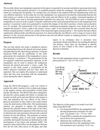
theta_10 = 15*(pi/180);
theta_20 = 135*(pi/180);
% Define Constant Variables
C1 = (Km1*Kg1)/Rm1;
C2 = (Km2*Kg2)/Rm2;
Jeq1 = (M1+M2)*(L1^2) + 2*M2*L1*L2*cos(theta_20) + M2*(L2^2) + Jm1*(Kg1^2);
Jeq2 = M2*(L2^2) + Jm2*(Kg2^2);
Beq1 = (Km1*Ke1*(Kg1^2))/Rm1;
Beq2 = (Km2*Ke2*(Kg2^2))/Rm2;
Keq1 = -(M1+M2)*sin(theta_10)*L1*g - M2*g*L2*sin(theta_10 + theta_20);
Keq2 = -M2*g*L2*sin(theta_10+theta_20);
% Find Gains
Kv1 = (2*damp1*n_freq1*Jeq1 - Beq1)/C1;
Kv2 = (2*damp2*n_freq2*Jeq2 - Beq2)/C2;
Kp1 = (Jeq1*(n_freq1^2)-Keq1)/C1;
Kp2 = (Jeq2*(n_freq2^2)-Keq2)/C2;
% Transfer Functions
Const1 = tf(C1*Kp1,[Jeq1 Beq1+C1*Kv1 Keq1+C1*Kp1]);
Const2 = tf(C2*Kp2,[Jeq2 Beq2+C2*Kv2 Keq2+C2*Kp2]);
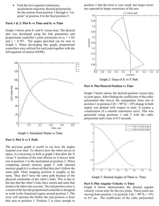
% Plot theta 1 and theta 2
step(Const1,'r');
hold on
step(Const2,'b');
hold off
legend('Theta 1','Theta 2')
%% Linear EOM (Question 1)
% Initialize
time(1) = 0;
dt = 0.005;
t_end = 0.5;
k = 1;
theta_1(1) = 15*(pi/180);
theta_2(1) = 135*(pi/180);
dtheta_1(1) = 0;
dtheta_2(1) = 0;
while time(k) < t_end
theta_1d(1) = 16*(pi/180);
theta_2d(1) = 136*(pi/180);
dtheta_1d(1) = 0;
dtheta_2d(1) = 0;
% Controls

9. e1 = theta_1d(1) - theta_1(k);
e2 = theta_2d(1) - theta_2(k);
ed1 = dtheta_1d(1) - dtheta_1(k);
ed2 = dtheta_2d(1) - dtheta_2(k);
V1(k) = Kp1*e1 + Kv1*ed1;
V2(k) = Kp2*e2 + Kv2*ed2;
% Find Acceleration
ddtheta(1) = (C1*V1(k)-Beq1*(dtheta_1(k)-dtheta_1(1))-Keq1*(theta_1(k)-theta_1(1)))/Jeq1;
ddtheta(2) = (C2*V2(k)-Beq2*(dtheta_2(k)-dtheta_2(1))-Keq2*(theta_2(k)-theta_2(1)))/Jeq2;
%dtheta(1) == 0
% Find next Velocity
dtheta_1(k+1) = dtheta_1(k) + ddtheta(1)*dt;
dtheta_2(k+1) = dtheta_2(k) + ddtheta(2)*dt;
% Find next Position
theta_1(k+1) = theta_1(k) + dtheta_1(k)*dt;
theta_2(k+1) = theta_2(k) + dtheta_2(k)*dt;
% Step
k = k + 1;
time(k) = time(k-1)+dt;
end
% Make all vectors same length
dtheta_1(k) = dtheta_1(k) + ddtheta(1)*dt;
dtheta_2(k) = dtheta_2(k) + ddtheta(2)*dt;
theta_1(k) = theta_1(k) + ddtheta(1)*dt;
theta_2(k) = theta_2(k) + ddtheta(2)*dt;
V1(k) = V1(k-1);
V2(k) = V2(k-1);
% Step
figure
step(Const1,'m');
hold on
step(Const2,'g');
plot(time,(theta_1-theta_1(1))*(180/pi),'r',time,(theta_2-theta_2(1))*(180/pi),'b');
legend('Theta 1 theory','Theta 2 theory','Theta 1 simulated','Theta 2
simulated','Location','southeast')
axis([0 0.5 0 1.4])
hold off
%% Non-Linear EOM (Question 2)
% Symbolic
syms Izz1 Izz2 M1 M2 L1 L2 th1a th2a dth1a dth2a g
syms Rm1 Rm2 V1 Nin2 Jm1 Jm2 Kg1 Kg2 Km1 Km2 Ke1 Ke2
% Initialize
time(1) = 0;
dt = 0.005;
t_end = 0.5;
k = 1;
% Mass Matrix
H(1,1) = Izz1+Izz2+M1*L1^2+M2*L1^2+2*M2*L1*L2*cos(th2a)+M2*L2^2+Jm1*Kg1^2;
H(1,2) = Izz2+M2*L1*L2*cos(th2a)+M2*L2^2;
H(2,1) = H(1,2);
H(2,2) = Izz2+M2*L2^2+Jm2*Kg2^2;
% Voltage and Gravity Matrix

10. V = M2*sin(th2a)*L1*L2*[-2*dth1a*dth2a-dth2a^2;dth1a^2]...
+[Ke1*Km1/Rm1*Kg1^2*dth1a ; Ke2*Km2/Rm2*Kg2^2*dth2a];
Grav = [M1*L1*cos(th1a)+M2*(L2*cos(th1a+th2a)+L1*cos(th1a));...
M2*L2*cos(th1a+th2a)]*g;
% full EOM: H * ddth + Vee + Gee = tau = vin*C* (Kp*e -Kv*Thdot)
Izz1=0;
Izz2=0;
% N-m-s^2—note: this is the motor armature inertia, already
% reflected thru the gear ratio
M1 = 0.035;
M2 = 0.067; % kg
L1 = 0.2;
L2 = 0.3; % m
Ke1 = 0.00767;
Ke2 = 0.0053;
Km1 = 0.00767;
Km2 = 0.0053;
Rm1 = 2.6;
Rm2 = 9.1;
Jm1 = 3.87e-7;
Jm2 = 6.8e-8;
Kg1 = 14;
Kg2 = 262;
g = 9.81;
H_inv =inv(H);
% Initial conditions;
TH1(1) = 15 * pi/180;
TH2(1) = 135 * pi/180;
DTH1(1) = 0;
DTH2(1) = 0;
while time(k) < t_end;
% desired location
th1D = 90 * pi / 180; % desired position in degrees
th2D = 10 * pi / 180; % desired position in degrees
dth1D = 0;
dth2D = 0;
v1(k)= Kp1 * ( th1D - TH1(k) ) + Kv1 * ( dth1D - DTH1(k));
v2(k)= Kp2 * ( th2D - TH2(k) ) + Kv1 * ( dth2D - DTH2(k));
Tau=[ Km1*Kg1/Rm1*v1(k); Km2*Kg2/Rm2*v2(k) ]; % generate the torque
tau1(k) = Tau(1); % record the torques
tau2(k) = Tau(2);
th1a = TH1(k);th2a=TH2(k);dth1a=DTH1(k);dth2a=DTH2(k);
DDTH = double(subs( H_inv*(Tau-V-Grav) ));
DDTH1(k) = DDTH(1);
DDTH2(k) = DDTH(2);
% acceleration: ddth = Hinv * (Tau-Vee-Grav);
% Integrate the full equations
DTH1(k+1)= DTH1(k)+ DDTH(1)*dt;
DTH2(k+1)= DTH2(k)+ DDTH(2)*dt;
TH1(k+1) = TH1(k)+ DTH1(k)*dt;
TH2(k+1) = TH2(k)+ DTH2(k)*dt;
% Extract x-y location
theta1temp = TH1(k);
theta2temp = TH2(k);
x(k) = double(subs(T0E(1,4)));
y(k) = double(subs(T0E(2,4)));

11. xj(k) = double(subs(T02(1,4)));
yj(k) = double(subs(T02(2,4)));
% Step
time(k+1)=time(k)+dt;
k=k+1;
end;
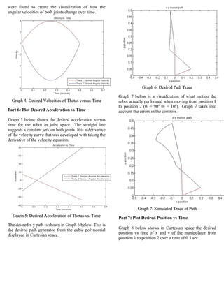
figure
plot(time,(TH1)*180/pi,'r-',time,(TH2)*180/pi,'b-');
xlabel('time, sec');
ylabel('joint angle,deg');
legend('Theta 1','Theta 2');
% Plot x-y path
figure
plot(x,y,'k-')
xlabel('x-position')
ylabel('y-position')
title('x-y motion path')
hold on
plot([0,xj(1)],[0,yj(1)],'r-')
plot([0,xj(length(xj))],[0,yj(length(yj))],'r-')
plot([xj(1),x(1)],[yj(1),y(1)],'b-')
plot([xj(length(x)),x(length(x))],[yj(length(y)),y(length(y))],'b-')
axis([-0.5 0.5 0 0.5])
%% Spline generation
% Create the spline from P1 to P2
%tend = 0.5;
dt = 0.001;
k = 1;
timef = t_end;
TH01 = 15*pi/180;
THf1 = 90*pi/180;
TH02 = 135*pi/180;
THf2 = 10*pi/180;
a0_1 = TH01;
a1_1 = 0;
a2_1 = 3/timef^2*(THf1 - TH01);
a3_1 = -2/timef^3*(THf1 - TH01);
a0_2 = TH02;
a1_2 = 0;
a2_2 = 3/timef^2*(THf2 - TH02);
a3_2 = -2/timef^3*(THf2 - TH02);
time(k) = 0;
while time(k) < t_end;
ddthD1(k) = a2_1 + 6*a3_1*time(k);
dthD1(k) = a1_1 + 2*a2_1*time(k) + 3*a3_1*time(k)^2;
thD1(k) = a0_1 + a1_1*time(k) + a2_1*time(k)^2 + a3_1*time(k)^3;
ddthD2(k) = a2_2 + 6*a3_2*time(k);
dthD2(k) = a1_2 + 2*a2_2*time(k) + 3*a3_2*time(k)^2;
thD2(k) = a0_2 + a1_2*time(k) + a2_2*time(k)^2 + a3_2*time(k)^3;

12. % Extract x-y location
theta1temp = thD1(k);
theta2temp = thD2(k);
x(k) = double(subs(T0E(1,4)));
y(k) = double(subs(T0E(2,4)));
xj(k) = double(subs(T02(1,4)));
yj(k) = double(subs(T02(2,4)));
k = k + 1;
time(k) = time(k - 1) + dt;
end;
ddthD1(k) = ddthD1(k - 1);
dthD1(k) = dthD1(k - 1);
thD1(k) = thD1(k - 1);
ddthD2(k) = ddthD2(k - 1);
dthD2(k) = dthD2(k - 1);
thD2(k) = thD2(k - 1);
% Plot the desired position vs time
figure
plot(time, thD1,'r-')
hold on
plot(time, thD2, 'b-')
legend('Theta 1 Desired Angle','Theta 2 Desired Angle')
hold off
% Plot the desired velocity vs time
figure
plot(time, dthD1,'r-')
hold on
plot(time, dthD2, 'b-')
legend('Theta 1 Desired Angular Velocity','Theta 2 Desired Angular Velocity')
hold off
% Plot the desired acceleration vs time
figure
plot(time, ddthD1,'r-')
hold on
plot(time, ddthD2, 'b-')
legend('Theta 1 Desired Angular Acceleration','Theta 2 Desired Angular Acceleration')
hold off
% Plot x-y path
figure
plot(x,y,'k-')
xlabel('x-position')
ylabel('y-position')
title('x-y motion path')
hold on
plot([0,xj(1)],[0,yj(1)],'r-')
plot([0,xj(length(xj))],[0,yj(length(yj))],'r-')
plot([xj(1),x(1)],[yj(1),y(1)],'b-')
plot([xj(length(x)),x(length(x))],[yj(length(y)),y(length(y))],'b-')
axis([-0.5 0.5 0 0.5])

13. %% Create the spline from P3 thru P4 to P5
% Initial Position
TH01i = 90*pi/180;
TH02i = 45*pi/180;
DTH1i = 0;
DTH2i = 0;
% Via Position
TH01v = 60*pi/180;
TH02v = 135*pi/180;
% DTH1v(1) = 0;
% DTH2v(1) = 0;
% Final Position
TH01f = 30*pi/180;
TH02f = 20*pi/180;
DTH1f = 0;
DTH2f = 0;
% Spline Equations
timef = 0.5;
a0_3a = TH01i;
a1_3a = 0;
a2_3a = (12*TH01v - 3*TH01f - 9*TH01i)/(4*timef^2);
a3_3a = (-8*TH01v + 3*TH01f + 5*TH01i)/(4*timef^3);
a0_3b = TH02i;
a1_3b = 0;
a2_3b = (12*TH02v - 3*TH02f - 9*TH02i)/(4*timef^2);
a3_3b = (-8*TH02v + 3*TH02f + 5*TH02i)/(4*timef^3);
a0_4a = TH01v;
a1_4a = (3*TH01f - 3*TH01i)/(4*timef);
a2_4a = (-12*TH01v + 6*TH01f + 6*TH01i)/(4*timef^2);
a3_4a = (8*TH01v - 5*TH01f - 3*TH01i)/(4*timef^3);
a0_4b = TH02v;
a1_4b = (3*TH02f - 3*TH02i)/(4*timef);
a2_4b = (-12*TH02v + 6*TH02f + 6*TH02i)/(4*timef^2);
a3_4b = (8*TH02v - 5*TH02f - 3*TH02i)/(4*timef^3);
k = 1;
clear time
time(k) = 0;
while time(k) < t_end
ddth1d(k) = 2*a2_3a + 6*a3_3a*time(k);
dth1d(k) = a1_3a + 2*a2_3a*time(k) + 3*a3_3a*time(k)^2;
th1d(k) = a0_3a + a1_3a*time(k) + a2_3a*time(k)^2 + a3_3a*time(k)^3;
ddth2d(k) = 2*a2_3b + 6*a3_3b*time(k);
dth2d(k) = a1_3b + 2*a2_3b*time(k) + 3*a3_3b*time(k)^2;
th2d(k) = a0_3b + a1_3b*time(k) + a2_3b*time(k)^2 + a3_3b*time(k)^3;
% Extract x-y location
theta1temp = th1d(k);
theta2temp = th2d(k);
xa(k) = double(subs(T0E(1,4)));
ya(k) = double(subs(T0E(2,4)));

14. xja(k) = double(subs(T02(1,4)));
yja(k) = double(subs(T02(2,4)));
k = k + 1;
time(k) = time(k - 1) + dt;
end
k = 1;
clear time
time(k) = 0;
% Spline 4-5
while time(k) < t_end
ddth1d(k) = 2*a2_4a + 6*a3_4a*time(k);
dth1d(k) = a1_4a + 2*a2_4a*time(k) + 3*a3_4a*time(k)^2;
th1d(k) = a0_4a + a1_4a*time(k) + a2_4a*time(k)^2 + a3_4a*time(k)^3;
ddth2d(k) = 2*a2_4b + 6*a3_4b*time(k);
dth2d(k) = a1_4b + 2*a2_4b*time(k) + 3*a3_4b*time(k)^2;
th2d(k) = a0_4b + a1_4b*time(k) + a2_4b*time(k)^2 + a3_4b*time(k)^3;
% Extract x-y location
theta1temp = th1d(k);
theta2temp = th2d(k);
xb(k) = double(subs(T0E(1,4)));
yb(k) = double(subs(T0E(2,4)));
xjb(k) = double(subs(T02(1,4)));
yjb(k) = double(subs(T02(2,4)));
k = k + 1;
time(k) = time(k - 1) + dt;
end
x = [xa xb];
y = [ya yb];
xj = [xja xjb];
yj = [yja yjb];
% Plot x-y path
figure
plot(x,y,'k-')
xlabel('x-position')
ylabel('y-position')
title('x-y motion path')
hold on
plot([0,xj(1)],[0,yj(1)],'r-')
plot([0,xj(0.5*length(xj))],[0,yj(0.5*length(yj))],'r-')
plot([0,xj(length(xj))],[0,yj(length(yj))],'r-')
plot([xj(1),x(1)],[yj(1),y(1)],'b-')
plot([xj(0.5*length(x)),x(0.5*length(x))],[yj(0.5*length(y)),y(0.5*length(y))],'b-')
plot([xj(length(x)),x(length(x))],[yj(length(y)),y(length(y))],'b-')
axis([-0.5 0.5 0 0.5])
%% Non-linear EOM P3-P5
% Initialize
time(1) = 0;

15. dt = 0.005;
t_end = 0.5;
k = 1;
% Initial conditions;
TH1(1) = 90 * pi/180;
TH2(1) = 45 * pi/180;
DTH1(1) = 0;
DTH2(1) = 0;
while time(k) < t_end;
% desired location
th1D = 60 * pi / 180; % desired position in degrees
th2D = 135 * pi / 180; % desired position in degrees
dth1D = 0;
dth2D = 0;
v1(k)= Kp1 * ( th1D - TH1(k) ) + Kv1 * ( dth1D - DTH1(k));
v2(k)= Kp2 * ( th2D - TH2(k) ) + Kv1 * ( dth2D - DTH2(k));
Tau=[ Km1*Kg1/Rm1*v1(k); Km2*Kg2/Rm2*v2(k) ]; % generate the torque
tau1(k) = Tau(1); % record the torques
tau2(k) = Tau(2);
th1a = TH1(k);th2a=TH2(k);dth1a=DTH1(k);dth2a=DTH2(k);
DDTH = double(subs( H_inv*(Tau-V-Grav) ));
DDTH1(k) = DDTH(1);
DDTH2(k) = DDTH(2);
% acceleration: ddth = Hinv * (Tau-Vee-Grav);
% Integrate the full equations
DTH1(k+1)= DTH1(k)+ DDTH(1)*dt;
DTH2(k+1)= DTH2(k)+ DDTH(2)*dt;
TH1(k+1) = TH1(k)+ DTH1(k)*dt;
TH2(k+1) = TH2(k)+ DTH2(k)*dt;
% Extract x-y location
theta1temp = TH1(k);
theta2temp = TH2(k);
xa_act(k) = double(subs(T0E(1,4)));
ya_act(k) = double(subs(T0E(2,4)));
xja_act(k) = double(subs(T02(1,4)));
yja_act(k) = double(subs(T02(2,4)));
% Step
time(k+1)=time(k)+dt;
k=k+1;
end;
% Initialize
time(1) = 0;
dt = 0.005;
t_end = 0.5;
k = 1;
% Initial conditions;
TH1(1) = 60 * pi/180;
TH2(1) = 135 * pi/180;
DTH1(1) = 0;
DTH2(1) = 0;
while time(k) < t_end;
% desired location
th1D = 30 * pi / 180; % desired position in degrees

16. th2D = 20 * pi / 180; % desired position in degrees
dth1D = 0;
dth2D = 0;
v1(k)= Kp1 * ( th1D - TH1(k) ) + Kv1 * ( dth1D - DTH1(k));
v2(k)= Kp2 * ( th2D - TH2(k) ) + Kv1 * ( dth2D - DTH2(k));
Tau=[ Km1*Kg1/Rm1*v1(k); Km2*Kg2/Rm2*v2(k) ]; % generate the torque
tau1(k) = Tau(1); % record the torques
tau2(k) = Tau(2);
th1a = TH1(k);th2a=TH2(k);dth1a=DTH1(k);dth2a=DTH2(k);
DDTH = double(subs( H_inv*(Tau-V-Grav) ));
DDTH1(k) = DDTH(1);
DDTH2(k) = DDTH(2);
% acceleration: ddth = Hinv * (Tau-Vee-Grav);
% Integrate the full equations
DTH1(k+1)= DTH1(k)+ DDTH(1)*dt;
DTH2(k+1)= DTH2(k)+ DDTH(2)*dt;
TH1(k+1) = TH1(k)+ DTH1(k)*dt;
TH2(k+1) = TH2(k)+ DTH2(k)*dt;
% Extract x-y location
theta1temp = TH1(k);
theta2temp = TH2(k);
xb_act(k) = double(subs(T0E(1,4)));
yb_act(k) = double(subs(T0E(2,4)));
xjb_act(k) = double(subs(T02(1,4)));
yjb_act(k) = double(subs(T02(2,4)));
% Step
time(k+1)=time(k)+dt;
k=k+1;
end;
x_act = [xa_act xb_act];
y_act = [ya_act yb_act];
xj_act = [xja_act xjb_act];
yj_act = [yja_act yjb_act];
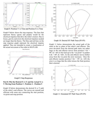
% Plot x-y path
figure
plot(x_act,y_act,'k-')
xlabel('x-position')
ylabel('y-position')
title('x-y motion path')
hold on
plot([0,xj_act(1)],[0,yj_act(1)],'r-')
plot([0,xj_act(0.5*length(xj_act))],[0,yj_act(0.5*length(yj_act))],'r-')
plot([0,xj_act(length(xj_act))],[0,yj_act(length(yj_act))],'r-')
plot([xj_act(1),x_act(1)],[yj_act(1),y_act(1)],'b-')
plot([xj_act(0.5*length(x_act)),x_act(0.5*length(x_act))],[yj_act(0.5*length(y_act)),y_act(0.5
*length(y_act))],'b-')
plot([xj_act(length(x_act)),x_act(length(x_act))],[yj_act(length(y_act)),y_act(length(y_act))]
,'b-')
axis([-0.5 0.5 -0.1 0.5])