This document is the thesis of Dmitriy Rivkin submitted in partial fulfillment of the requirements for a Master of Science degree in Computer Engineering from the University of California, Santa Cruz. The thesis investigates optimal control techniques for minimum energy attitude maneuvers of CubeSats using reaction wheels. It formulates the optimal control problem, develops algorithms to solve for optimal trajectories, and analyzes the performance of the optimal trajectories through simulations and hardware experiments on a CubeSat testbed. The thesis contributes to advancing optimal control methods for efficient attitude control of small satellites.


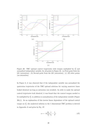
![27 Many PRC optimal control trajectories plotted together. (a) tf var-
ied, brighter line corresponds to longer maneuver time. (b) Reaction
wheel MOI varied, brighter line corresponds to smaller reaction wheel. 47
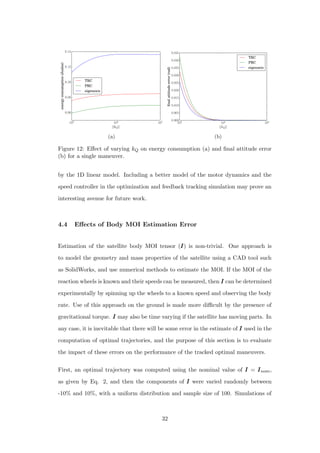
28 Energy consumption broken down by the three terms of Eq. 23 for
TRC and PRC optimal solutions as maneuver angle is varied. . . . . 48
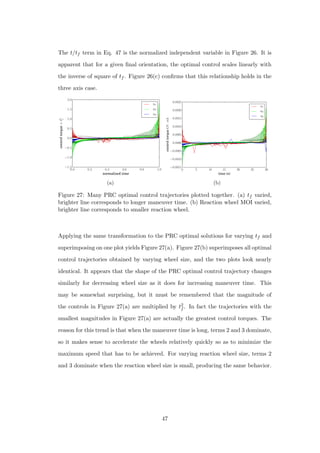
29 Percent energy reduction of PRC over TRC as the maneuver angle
varies for three values of tf . . . . . . . . . . . . . . . . . . . . . . . . 49
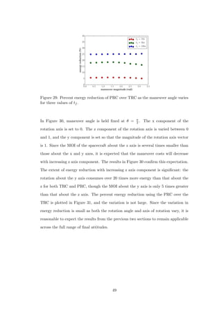
30 Energy consumption broken down by the three terms of Eq. 23 for
TRC and PRC optimal solutions as the z component of the rotation
axis is varied. . . . . . . . . . . . . . . . . . . . . . . . . . . . . . . . 50
31 Percent energy reduction of PRC over TRC as the z component of
the rotation vector varies. . . . . . . . . . . . . . . . . . . . . . . . . 50
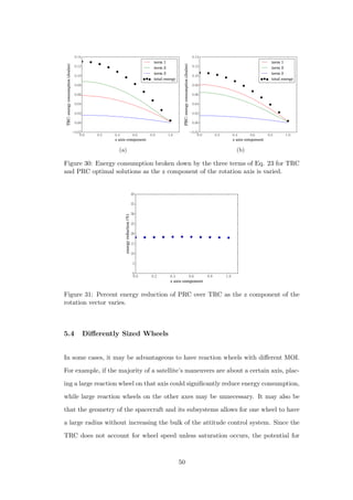
32 Variation of maneuver angle for three reaction wheel configurations.
Wheel MOI are (in kg · m2 × 10−5): different wheels = [10 1 1],
small wheels = [1 1 1], large wheels = [10 10 10]. (a) Percent energy
reduction using PRC over TRC. (b) Energy consumption of PRC
optimal solutions. . . . . . . . . . . . . . . . . . . . . . . . . . . . . . 51
33 Optimal body rate trajectories for control system with differently
sized reaction wheels. (a) TRC optimal θ = π
2 . (b) PRC optimal
θ = π
2 . (c) TRC optimal θ = π. (d) PRC optimal θ = π. . . . . . . . 53
34 Variation of z component of rotation axis for three reaction wheel
configurations. Wheel MOI are (in kg · m2 × 10−5): different wheels
= [10 1 1], small wheels = [1 1 1 ], large wheels = [10 10 10]. (a)
Percent energy reduction of PRC over TRC solutions, θ = π
2 . (b)
Energy consumption of PRC optimal solutions, θ = π
2 . (c) Percent
energy reduction of PRC over TRC solutions, θ = π. (d) Energy
consumption of PRC optimal solutions, θ = π. . . . . . . . . . . . . 54
35 PRC optimal body rate trajectories with θ = π. (a) z = 0.6. (b)
z = 0.7. . . . . . . . . . . . . . . . . . . . . . . . . . . . . . . . . . . 55
viii](https://image.slidesharecdn.com/2e1917f8-359f-47e1-92a7-a1899f984d19-160719215916/85/Dmitriy-Rivkin-Thesis-8-320.jpg)

![1 Introduction
Cubesats are very small, very low-cost satellites about the size of a loaf of bread,
that are affordable to a much broader user base than conventional (normal scale)
satellites, including universities [15], start-ups [20], and even non-government space
exploration societies[32]. They are comparable to modern smartphones in that they
are both compact and inexpensive packages that provide access to technology previ-
ously too expensive for most to afford. In both cases the availability of technology in
an affordable package allows for novel usage modalities. For example, the QB50 mis-
sion used a swarm of Cubesats making measurements upon atmospheric re-entry to
study the upper atmosphere [15], a mission that would not have been economically
feasible using full scale satellites. Unfortunately, the low pricetag is the result of ex-
treme size, weight, and power (SWaP) constraints. The severity of these constraints
motivates the optimization of spacecraft components.
One component that can take up a significant fraction of the SWaP budget is the at-
titude control system. Broadly speaking, the actuation torque a controller is capable
of producing is proportional to its size. Light, compact actuators, such as magnetic
torquers (electromagnetic coils which produce a control torque through interaction
with the Earth’s magnetic field), are capable of stabilizing the spacecraft against the
small disturbance torques present in low Earth orbit, but cannot maneuver quickly
or achieve high pointing accuracy. A class of higher performing, bulkier actuators in-
cludes includes cold gas thrusters, control moment gyros (CMG), and reaction wheel
arrays (RWA). Cold gas thrusters consume fuel which needs to be stored and cannot
be recovered. CMGs are mechanically complex, as they require an actuated gimble.
Reaction wheel arrays are mechanically simple and do not consume any fuel, making
them a popular attitude control method, especially for small satellites. However, all
active attitude control systems require additional volume, power, complexity, and
computation.
The intent of this work is to help RWA designers increase the efficiency of their
1](https://image.slidesharecdn.com/2e1917f8-359f-47e1-92a7-a1899f984d19-160719215916/85/Dmitriy-Rivkin-Thesis-13-320.jpg)
![systems through trajectory optimization. The efficacy and value of this approach
depend on the myriad specifics of the mission. However, there are relationships
between certain key control system parameters, energy consumption, and the energy
saving potential of trajectory optimization. This work explores these relationships
to help designers develop an intuition for some ways in which they can reduce the
energy consumption of their systems, and potentially the weight and volume as well.
The solutions presented in this work are the results of analysis, simulation, and
optimization of a hypothetical system with physical parameters similar to those of
a 3 unit Cubesat (defined by the Cubesat standard [10]) with three reaction wheels.
We believe that many of the trends identified and techniques used in this work are
applicable to the design of larger spacecraft as well. To obtain maximum benefit,
designers should adapt the analysis to reflect the specifics of their systems.
1.1 Reaction Wheel Array Attitude Controller
The RWA is a momentum exchange device. A momentum wheel is attached to
the rotor of an electric motor, the stator of which is coupled to the body of the
satellite. When the motor applies a torque to the reaction wheel, an equal and
opposite torque is exerted on the satellite body, producing an angular acceleration.
A minimum of three reaction wheels allow for full control in three axes. RWAs with
three wheels are normally arranged orthogonally. On larger satellites, the RWA often
consists of a tetrahedral array of four reaction wheels; this arrangement is robust
to failure of any one of the reaction wheels. However, due to severe volume and
weight constraints, short orbital lifespans, and the relatively low cost of replacing
a malfunctioning satellite, Cubesat RWAs usually only have three wheels. Because
all torque is produced only by electric motors, RWA attitude control consumes only
electrical energy, which is generated by solar panels covering the satellite body.
RWAs do not produce external torques, i.e. the angular momentum of the satellite
body / RWA system remains constant even as the wheels and satellite accelerate in
opposite directions by the law of conservation of angular momentum. In order to
2](https://image.slidesharecdn.com/2e1917f8-359f-47e1-92a7-a1899f984d19-160719215916/85/Dmitriy-Rivkin-Thesis-14-320.jpg)
![keep the satellite stable in the presence of external torque, the RWA must accelerate,
absorbing the extra momentum. If no action is taken to dump this extra momentum,
the RWA will eventually saturate, and will no longer be able to exert the necessary
control torques on the body. To avoid saturation, the RWA must be coupled with
a controller that is capable of producing a torque against the external environment,
in order to dump the momentum. Usually this secondary controller is based on
magnetic torquers. While not capable of performing fast maneuvers on their own,
the electromagnetic torquers can produce enough torque to compensate for external
disturbances (e.g. atmospheric drag, solar wind, and gravity gradient torque).
For detailed background discussion of RWAs, see [36].
1.1.1 Momentum Wheels
It is desirable for momentum wheels to have a large Moment of Inertia (MOI) about
their rotational axes. The higher the MOI of the wheels, the higher the maximum
body angular rate the RWA can produce, and the more external torque the system
can absorb before saturation occurs. Another advantage of high reaction wheel
MOI stems from the fact that Cubesats are often deployed with a non-zero angular
body rate, a scenario known as tumbling. Reaction wheels of sufficient MOI can de-
tumble a satellite by absorbing the angular momentum of the spacecraft. All of these
advantages stem from the fact that wheels with higher MOI can absorb more angular
momentum before saturating. Higher-MOI reaction wheels also require lower energy
consumption during large angle attitude maneuvers, as will be shown in Chapter 5.
The moment of inertia of a disk about its rotational axis can be computed as follows:
MOI =
1
2
mr2
(1)
where m and r are the mass and radius of the disk. Examination of Eq. 1 reveals the
cost of high-MOI reaction wheels: higher MOI either requires more mass or a larger
radius. Increasing the radius makes the wheel less compact, resulting in a greater
3](https://image.slidesharecdn.com/2e1917f8-359f-47e1-92a7-a1899f984d19-160719215916/85/Dmitriy-Rivkin-Thesis-15-320.jpg)
![system volume. Increasing mass is also undesirable, due to the strict weight budget.
Because reaction wheels with higher MOI tend to be heavier and more voluminous,
they are sometimes referred to simply as “larger” reaction wheels in the remainder
of this document. As demonstrated in this work, a RWA should have the smallest
wheels that meet performance specifications and energy consumption limits.
1.1.2 Motors and Motor Drivers
Brushless DC (BLDC) motors, sometimes also known as permanent magnet syn-
chronous motors (PMSM), are used to drive the reaction wheels. Compared to DC
motors, BLDCs are more efficient and do not produce carbon dust, which is espe-
cially beneficial in a weightless, electronics-dense environment. Unlike DC motors,
which are mechanically commutated by carbon brushes, BLDCs are electronically
commutated; the user must control the stator current to produce the desired torque.
This control is achieved using switch-mode electronics and a micro-controller. For
more on BLDC motors and control, refer to [24]. If the stator currents of the mo-
tor’s three phases, as well as the position of the rotor, can be accurately measured,
a sophisticated motor control algorithm can precisely produce the desired control
torque. Cubesat motor drivers are often less sophisticated, and are better suited to
speed control than torque control. Cubesats motor drivers are also often incapable
of regenerative braking, a mode of operation in which kinetic rotational energy of the
reaction wheel is converted back into stored battery energy, as adding regenerative
braking capabilities increases the complexity of the satellite’s power system.
1.2 Eigenaxis Maneuvers
A convenient and popular method of computing trajectories for large angle attitude
maneuvers is to constrain the satellite to rotation about a single axis called the
eigenaxis [38]. The eigenaxis maneuver takes the shortest kinematic path between
two attitudes. An angular body rate profile is then chosen to ensure that the satellite
4](https://image.slidesharecdn.com/2e1917f8-359f-47e1-92a7-a1899f984d19-160719215916/85/Dmitriy-Rivkin-Thesis-16-320.jpg)
![reaches the desired attitude within the required time. The shape of this profile has
a significant effect on the energy consumption of the maneuver. In order to evaluate
the improvements in energy consumption afforded by trajectory optimization, the
eigenaxis maneuver is used as a baseline. The angular velocity profile is chosen such
that the velocity increases at a constant rate until the midpoint, and then decreases
at the same rate until the endpoint, so that the satellite comes to rest at the desired
attitude. Optimization of the velocity profile is beyond the scope of this work, but
the constant acceleration approach produces energy consumption that is on the same
order of magnitude as that of the energy optimal maneuvers, in contrast with the
energy consumed by time optimal maneuvers, which are about 50-100 times more
energetically costly.
1.3 Related Work
1.3.1 Trajectory Optimization
Trajectory optimization is concerned with the computation of a state/control tra-
jectory pair that minimizes some cost metric. The cost metric in this type of opti-
mization depends on variables which are themselves functions of time, thus the cost
metric is referred to as a cost functional; a function of functions. With the excep-
tion of [22], the following works optimize a cost functional which depends only on
control torque. Some authors refer to this kind of optimization as energy optimal,
while other use the term “torque optimal”, which is more accurate. [12] computed
trajectories that minimized the integral of the sum of squares of control torques for
an attitude controller with cold gas thrusters and magnetic torquers. [19] minimized
the integral of control torque magnitude, without modeling the actuator producing
the torque, while accounting for external disturbances. [21] modeled the dynamics
of the reaction wheel array, and computed optimal trajectories in the presence of
path constraints, minimizing a cost functional that included terms accounting for
both maneuver time and control torque magnitude. [22] optimized a model-based
5](https://image.slidesharecdn.com/2e1917f8-359f-47e1-92a7-a1899f984d19-160719215916/85/Dmitriy-Rivkin-Thesis-17-320.jpg)
![cost functional which more accurately modeled the energy losses of the RWA, and
demonstrated that the energy cost of the optimal maneuver is inversely proportional
to maneuver time by constructing a Pareto-optimal curve of maneuver time versus
energy consumption. This is the only discussion of the effect of optimization param-
eters on the minimum energy trajectory that we are aware of. [22] also computed
time-optimal maneuvers with energy constraints, as well as energy optimal eigenaxis
trajectories. Other works tend to focus on obtaining solutions to a single, specific
problem. Bedrossian’s large angle maneuver of the international space station using
only CMGs is the best known example of spacecraft attitude trajectory optimization
[6]. It is dissimilar from the other work mentioned above in that its main objective
was to avoid saturation of the CMGs due to external torques during a maneuver.
Saturation of Cubesat RWAs occurs on a significantly longer time scale than that
of a single maneuver, and can be compensated for with magnetic torquers. Apart
from [19], these works focus on satellites much larger than Cubesats.
All of the work above applied pseudospectral optimal control methods to compute
trajectories numerically. The same methods are also often applied to compute time
optimal trajectories as well. In fact, there is a large volume of work on minimum time
trajectory optimization of satellite attitude maneuvers [31],[8],[23],[14],[13]. Since
there exists a trade-off between time and energy in the satellite reorientation problem
[22], time-optimal maneuvers tend to be energetically expensive. Notably, however,
the time optimal work of [18] illustrates a way in which optimal attitude maneuvers
for RWAs computed using pseudospectral optimal control methods can be imple-
mented in practice. Maneuvers are computed on the ground and uploaded to an
imaging satellite. The quaternion attitude trajectories are tracked using a propor-
tional feedback control law. A significant improvement over eigenaxis trajectories
was demonstrated.
6](https://image.slidesharecdn.com/2e1917f8-359f-47e1-92a7-a1899f984d19-160719215916/85/Dmitriy-Rivkin-Thesis-18-320.jpg)
![1.3.2 Torque Allocation
The torque allocation problem arises when the RWA has more than three wheels.
In this case, there are an infinite number of combinations of individual reaction
wheel torques that produce the desired net control torque on the satellite body,
and the problem is choosing the combination that minimizes energy consumption.
The desired control can be computed via trajectory optimization, or by a feedback
controller tracking an eigenaxis trajectory. Examples of such work include [9],[39],
and [30]. The torque allocation problem is not closely related to the trajectory opti-
mization problem, but is mentioned here because solutions to the torque allocation
problem are sometimes referred to as energy optimal or power optimal.
1.4 Contributions
The following is an enumeration of work presented in this thesis:
1. The model based cost functional in [22] is adapted to model the non-regenerative
braking case, and resulting numerical challenges are overcome using approxi-
mation and problem reformulation. The benefits of optimization with respect
to this complex cost functional rather than a simpler, more convenient cost
are evaluated extensively.
2. An efficient method for computation of near optimal solutions is proposed.
This method is based on linear interpolation of precomputed solutions.
3. Relationships between parameter values, energy costs, and the utility of trajec-
tory optimization are explored. The parameters investigated include reaction
wheel MOI, final attitude, and maneuver time. Understanding of these rela-
tionships may aid Cubesat designers in making appropriate tradeoffs.
7](https://image.slidesharecdn.com/2e1917f8-359f-47e1-92a7-a1899f984d19-160719215916/85/Dmitriy-Rivkin-Thesis-19-320.jpg)
![Unless otherwise specified:
III =
248 0.21 0.61
0.21 248 0.61
0.61 0.61 49
× 10−4
kg · m2
(2)
Iw = 2.2 × 10⁻⁵
kg · m2
(3)
where III is the MOI tensor of the satellite body and Iw is the MOI of the reaction
wheels about their axes of rotation. Unless otherwise specified, all three reaction
wheels have the same MOI. The BLDC motors are 12 volt Faulhaber 2610s [3] with
the following parameters:
Ra = 28.2 Ω (4)
kt = 1.81 × 10⁻²
N · m/A (5)
µ = 1.29 × 10⁻⁷
N · m/(rad/s) (6)
where Ra is the armature resistance, kt is the motor torque constant, and µ is the
rotor dynamic friction coefficient. Since the wheels operate in the vacuum of space,
the only source of friction is the motor bearings. The value of ke, the motor electrical
constant, is equal to kt when both are expressed in S.I. units.
The maximum speed of the motors is 650 rad/s. The maximum torque production is
dependent on the motor speed. However, a constant torque limit of 3.0×10⁻³ N·m is
used in optimization and simulation since this level of torque production is achievable
at all speeds. In practice, for most problems, the magnitude of energy optimal
control torque trajectories stays well below the limits, since effecting large torques
consumes large quantities of energy. Saturation only occurs when the time allotted
for a maneuver is close to the minimum feasible time (see Chapter 5).
9](https://image.slidesharecdn.com/2e1917f8-359f-47e1-92a7-a1899f984d19-160719215916/85/Dmitriy-Rivkin-Thesis-21-320.jpg)
![2.2 Optimal Control Problem Formulation
To enable formulation as an optimal control problem, relevant physical quantities
must be cast as state and control variables. Notation is adopted from [29], where a
boldface font indicates a column vector.
xxx is the state vector, containing all quantities with dynamic constraints. uuu is the
control vector, containing quantities with algebraic constraints only. All quantities
contained in xxx and uuu are time varying, but (t) notation is dropped for compactness,
except when it is necessary to specify a value of xxx or uuu at some exact instant.
The vector uuu is comprised of the three reaction wheel motor torques (uuu = [τ1 τ2 τ3]T ).
The vector xxx contains the angular rate of the satellite body frame relative to the
inertial frame (ωωω = [ωx ωy ωz]T ), the angular rates of the three reaction wheels about
their spin axes with respect to the satellite body frame (ωwωwωw = [ωw,1 ωw,2 ωw,3]T ),
and the unit quaternion expressing the orientation of the body frame relative to the
inertial frame (qqq = [q0 q1 q2 q3]T ). In summary, xxx = [ωωωT ωwωwωw
T qqqT ]T .
Any attitude can be represented as a rotation by a certain angle around a single axis.
The unit quaternion is a vector with four entries, containing information about the
axis and and the angle of rotation. The unit attitude quaternion definition is given
by Eq. 7, where eee = [ex ey ez]T is the unit vector expressing the axis of rotation,
and θ is the angle of rotation.
qqq =
cos(θ
2)
exsin(θ
2)
eysin(θ
2)
ezsin(θ
2)
(7)
The magnitude of a quaternion is given by Eq. 8. The unit attitude quaternion has
10](https://image.slidesharecdn.com/2e1917f8-359f-47e1-92a7-a1899f984d19-160719215916/85/Dmitriy-Rivkin-Thesis-22-320.jpg)
![a magnitude of 1.
||qqq|| = qqqTqqq (8)
With the states and controls defined, the optimal control problem is formulated as
follows:
Minimize cost functional J =
tf
t0
g(xxx,uuu) dt (9)
Subject to : ˙x˙x˙x = fff(xxx,uuu) (10)
xxx(t0) = x0 (11)
xxx(tf ) = xf (12)
uL ≤ uuu ≤ uU (13)
xL ≤ xxx ≤ xU (14)
t0 and tf fixed (15)
qqq = 1 (16)
2.2.1 Constraints
Equations 10 - 16 specify constraints that must be satisfied by the solution. If no
solution can be found that satisfies all the constraints, the problem is called infeasi-
ble. Eq. 10 requires that the solution respects the dynamics of satellite, described
by the set of first order differential equations given below. Eq. 11 initializes the
state vector. For all the solutions in this document, the body rate and reaction
wheel speeds are all initialized at 0, and qqq(t0) = [1 0 0 0]T . Eq. 12 constrains the
final state, where ωωω(tf ) = [0 0 0]T , and qqq(tf ) specifies the required final attitude.
The final reaction wheel rates are not constrained, but because there are only three
reaction wheels and disturbance torques are neglected, the reaction wheels are effec-
tively constrained to be stationary at tf by the dynamics. Eq. 13 is the algebraic
constraint on control, and enforces motor torque limits. Eq. 14 is the algebraic state
11](https://image.slidesharecdn.com/2e1917f8-359f-47e1-92a7-a1899f984d19-160719215916/85/Dmitriy-Rivkin-Thesis-23-320.jpg)
![constraint, wherein the maximum reaction wheel speed is limited to the maximum
speed supported by the motors. Eq. 14 does not constrain ωωω and qqq. Eq. 15 fixes
the initial and final times. By convention, t0 = 0. Unless it is otherwise specified,
tf = 30s for the solutions presented in this document. Finally, Eq. 16 is a path
constraint, requiring that that qqq remains a unit quaternion at all times.
The spacecraft dynamics, fff(xxx,uuu), are derived in [18] and given below:
˙ωωω
˙ωωωw
= ΓΓΓ−1
−ωωω × (IωIωIω + 3
i=1 aaaiIw,iωωωw,i + aaaiIw,iaaaT
i ωωω)
uuu
ΓΓΓ =
III + 3
i=1 aaaiIw,iaaaT
i aaa1Iw,1 aaa2Iw,2 aaa3Iw,3
Iw,1aaaT
1 Iw,1 0 0
Iw,2aaaT
2 0 Iw,2 0
Iw,3aaaT
3 0 0 Iw,3
˙qqq =
1
2
qqq ⊗
0
ωωω
where III is the MOI tensor of the spacecraft body, and Iw,i is the MOI of reaction
wheel i about its axis of rotation. The vector aaai expresses the orientation of the axis
of rotation of reaction wheel i with respect to the body frame. ⊗ is the quaternion
multiplication operator.
2.3 Running Cost
While J in Eq. 9 is known as the cost functional, g(xxx,uuu) is called the running cost. In
contrast with time minimization, where the choice of cost functional is obvious, the
running cost in energy minimization should ideally reflect the power consumption
of the system, the time integral of which is energy. Power consumption is highly
system dependent, and may be challenging to model. A running cost based on a
high fidelity power model may also not be well suited to optimization, and produce
12](https://image.slidesharecdn.com/2e1917f8-359f-47e1-92a7-a1899f984d19-160719215916/85/Dmitriy-Rivkin-Thesis-24-320.jpg)
![significant numerical challenges. Therefore, a convenient approximation for power
consumption is the sum of squares of control torque, uuuTuuu, referred to as the torque
running cost (TRC) in the remainder if this document. This quadratic running cost
is smooth (infinitely differentiable over its whole domain) and convex, making it very
well suited to numerical optimization. It also requires no modeling of loss sources.
However, trajectories which are optimal with respect to this convenient running cost
do not minimize energy consumption. This motivates the formulation of a power
model based running cost.
2.4 Power Model
Ib
−
+
Vb
Ra
Rf
If
+
−Vm
Im
Figure 2: Circuit diagram of battery, drive electronics, and motor.
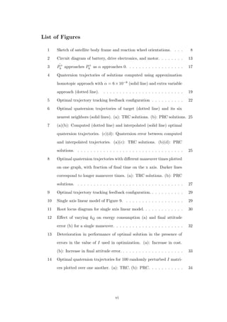
The following modeling and analysis, up to Eq. 23, are similar to those presented
in [22]. The battery, drive electronics, and motor of a single reaction wheel are
modeled by the circuit diagram in Figure 2. It is assumed that the drive electronics
will supply the correct amount of current to produce the commanded motor torque,
thus the battery and drive electronics are modeled by a current source with current
Ib and voltage Vb. Ra is the armature resistance of the motor. Vm is the back
electromotive force (EMF) produced by the rotation of the motor. The back EMF is
linearly proportional to the wheel speed, ωw, through the motor’s electrical constant,
ke. Im is the torque producing current, linearly proportional to the control torque,
u, through the motor’s torque constant, kt. Rf models the power dissipation due
to dynamic friction. If is the current required to compensate for dynamic friction
13](https://image.slidesharecdn.com/2e1917f8-359f-47e1-92a7-a1899f984d19-160719215916/85/Dmitriy-Rivkin-Thesis-25-320.jpg)
![power to be negative, a mode of operation known as regenerative braking. This
occurs when the deceleration demanded of the motor is less than it would be if the
battery were removed and the terminals shorted together.
Eq. 23 models battery power losses of a system capable of perfect bidirectional
power flow (regenerative braking). However, many Cubesats are not equipped with
a power system capable of handling reverse power flow, and this power is dissipated
as heat. Eq. 24 models the nonregenerative braking case.
P+
b =
Pb, if Pb > 0
0, otherwise
(24)
The model based running cost, hereafter referred to as the power running cost (PRC),
for the nonregenrative braking case is obtained by adding the power consumption
of all three reaction wheels:
PRC =
3
i=1
P+
b,i (25)
In the rest of this work, all quantification of energy consumption is implemented by
numerically integrating Eq. 25 from t0 to tf .
2.5 Solving the Optimal Control Problem
A Legendre pseudospectral method is used to solve the optimal control problem [27].
The pseudospectral approach is a direct method, meaning that the continuous time
problem is discretized and solved numerically as a parameter optimization problem.
In contrast, indirect methods apply Pontryagin’s principle to the problem to produce
a set of differential equations, the solution of which yields the optimal solution to
the original problem [29]. Unlike other direct methods, which make local discretiza-
tions, pseudospectral methods approximate the trajectory of a variable with a single
polynomial. Constraints are enforced at collocation points; discrete instances in
15](https://image.slidesharecdn.com/2e1917f8-359f-47e1-92a7-a1899f984d19-160719215916/85/Dmitriy-Rivkin-Thesis-27-320.jpg)
![time at which the constraints are evaluated. A Legendre pseudospectral method
uses the Legendre polynomials [37] as a basis for construction of the approximating
polynomial. The collocation points are arranged in a Legendre-Gauss-Lobatto grid
[16]. For a review of pseudospectral optimal control, see [28].
PSOPT is an open source optimal control package that uses a Legendre pseudospec-
tral method to convert the problem into a nonlinear programming (NLP) problem
[5], which is then solved by the NLP solver IPOPT (Interior Point OPTimizer) [34].
IPOPT, in turn, uses one of a number of available linear solvers to obtain a solu-
tion. PSOPT is a fast solver because it uses the ADOL-C (Automatic Differentiation
by OverLoading in C++) library [35] in order to compute requisite Jacobian and
Hessian matrices automatically, in contrast with numerical perturbation methods.
The solutions produced by PSOPT consist of the values of the state and control
variables at the collocation points. Methods that allow the use of these trajectories
to improve the maneuvering of a real satellite are discussed in the following chapter.
2.6 Numerical Challenges
Numerical optimal control solvers are sensitive to a number of optimization param-
eters and properties of the cost functional. Improper choice of these parameters, or
a poor problem formulation, results in divergence, or slow convergence, of the opti-
mization algorithm. Just obtaining a feasible solution may require a fair amount of
tuning. This work is concerned with the computation of large numbers of solutions
to varying problems, so it is critical to establish a robust computational approach
which will produce solutions under variable conditions.
2.6.1 Non-Smoothness of PRC
Attempting to solve the problem with the running cost given in Eq. 25 fails to
produce a solution. This is because most nonlinear programming (NLP) methods
16](https://image.slidesharecdn.com/2e1917f8-359f-47e1-92a7-a1899f984d19-160719215916/85/Dmitriy-Rivkin-Thesis-28-320.jpg)
![assume that the running cost is continuously differentiable with respect to states
and controls. A cost functional with a running cost which violates this assumption
often results in divergence or slow convergence of the solution [7]. The discontinuity
of the derivative of the PRC cost at zero produces unwanted behavior. A smoothing
approximation of the running cost can be used to obtain an approximate solution:
ˆP+
b =
1
2
( P2
b + α + Pb) , α > 0 (26)
As the approximation parameter, α, approaches 0, ˆP+
b approaches P+
b , as illustrated
by Figure 3. Choosing a high value results in a running cost that is very well suited
to optimization, but not very closely representative of the physical truth, while a
low value produces an accurate running cost that shares the numerical difficulties of
the original. Therefore, α should be chosen to be the smallest value that produces a
solution. To obtain the best results, a homotopic approach can be applied, where a
solution is computed for a certain value of α, and then that solution is used as the
initial guess in the next iteration, with a lower α value. Compared to a cold start,
where the initial guess is far from the optimal, this method decreases the minimum
α value that yields a solution.
−4 −2 0 2 4
Pb
0
1
2
3
4
5
6
7
8
9
ˆP+
b , α = 100
ˆP+
b , α = 10
ˆP+
b , α = 1
P+
b
Figure 3: ˆP+
b approaches P+
b as α approaches 0.
17](https://image.slidesharecdn.com/2e1917f8-359f-47e1-92a7-a1899f984d19-160719215916/85/Dmitriy-Rivkin-Thesis-29-320.jpg)
![Unfortunately, the homotopic method is slow, since it requires the computation of
a series of optimal trajectories.
Another way to deal with nonsmoothness of the running cost is to reformulate it
as a constraint through the addition of variables. This approach is outlined in [29]
for dealing with L1 optimal control problems, where an absolute value function is
present in the running cost. For each reaction wheel, a single variable, zi, is added
to the problem formulation. These additional variables have algebraic constraints
only, and are therefore treated by the solver the same way as controls. The PRC
can then be rewritten using path constraints on zi as follows:
zi − Pb,i ≥ 0 (27)
zi ≥ 0 (28)
PRC =
3
i=1
zi (29)
In Eq.s 27 and 28, zi is constrained to be greater than or equal to both Pb,i and 0.
In Eq. 29, the running cost is defined as the sum of all zi. In an optimal solution,
when Pb,i is positive zi = Pb,i, since increasing zi above its minimum allowable value
would only increase the cost. When Pb,i is negative, zi = 0 for the same reason.
Thus, the zeroing of the negative part of the power is reformulated as as a set of
constraints on zi, which solvers are better equipped to deal with. The success of
this approach depends on the linear solver used by IPOPT. The best performance is
achieved with the HSL MA57 solver [1], and solution time is comparable to that for
the TRC (which is relatively independent of linear solver). Use of HSL MA27 [1] and
MUMPS [4] linear solvers also yields a solution, but takes several times longer. Use
of HSL MA77, HSL MA86, or HSL MA96 [1] does not produce a feasible solution
in a reasonable amount of time.
Figure 4 shows solutions obtained using both approaches. There are some slight but
noticeable differences between these two trajectories, and the homotopic approach
consumes about 2% more energy than the additional variable approach. This is
18](https://image.slidesharecdn.com/2e1917f8-359f-47e1-92a7-a1899f984d19-160719215916/85/Dmitriy-Rivkin-Thesis-30-320.jpg)
![0 5 10 15 20 25 30
time (s)
−0.2
0.0
0.2
0.4
0.6
0.8
1.0
quaternion
q0
q1
q2
q3
Figure 4: Quaternion trajectories of solutions computed using approximation homo-
topic approach with α = 6 × 10⁻⁸ (solid line) and extra variable approach (dotted
line).
due to the fact that the former approximates the PRC, while the latter evaluates
it exactly. Due to its superiority in performance and computational efficiency, the
extra variable approach is used to generate the rest of the PRC solutions in this
document.
2.6.2 Scaling
In his book on numerical optimal control [7], J.T. Betts has the following to say
on the subject of scaling: “Scaling affects everything! Poor scaling can a make a
good algorithm bad. Scaling changes the convergence rate, termination tests, and
numerical conditioning.” He then offers some guidelines on how to scale problems,
but in general choosing a scaling method is an iterative process. In the simplest
terms, scaling is choosing custom units for time, states, controls, and the objective
function. Direct optimal control is a numerical method, therefore the performance
of algorithms depends on the numerical values of the variables. PSOPT provides
automatic scaling routines, outlined in the user manual [5], based on the recommen-
dations in [7], which proved to be sufficient for some, but not all, problems solved in
this work. In order to increase reliability, PSOPT’s automatic scaling routines were
augmented for some of the variables.
19](https://image.slidesharecdn.com/2e1917f8-359f-47e1-92a7-a1899f984d19-160719215916/85/Dmitriy-Rivkin-Thesis-31-320.jpg)
![control trajectory as input.
3 Optimal Control in Practice
Computation of optimal solutions is not enough: they must be executed by the
satellite to be valuable. Since the solutions are based on an imperfect model, using
the computed optimal control trajectories to control the satellite directly is likely
to yield significant errors. For increased robustness, the optimal solution is tracked
using a feedback controller. Additional challenges stem from the fact that optimiza-
tion is computationally expensive, and generally infeasible to perform aboard the
satellite. Solutions can be computed on the ground and radioed up to the satellite,
but this is undesireable since it produces communications overhead, and reduces the
ability of the satellite to operate independently. Another approach is to precompute
a bank of solutions before launch, and use these solutions to reduce computational
burden on the satellite hardware.
3.1 Optimal Trajectory Tracking
Perfect modeling of the satellite and controller dynamics is highly improbable, so
using the computed motor speeds or torques as input to the controller directly
would produce a significant amount of error in the execution, especially in the final
attitude. The solution is to use a feedback controller to track the computed attitude
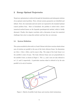
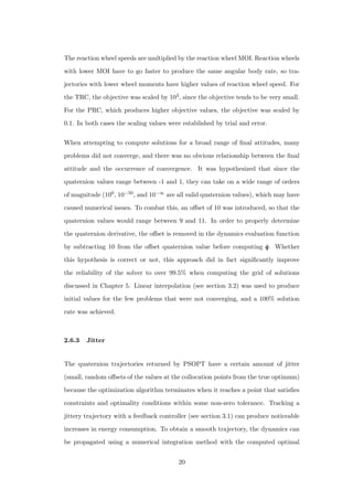
trajectory. This is a common approach in practical optimal control [6][18]. Figure 5
presents a block diagram of the tracking controller.
The input to the feedback controller at time t is the value of desired attitude quater-
nion at that time. qqqe is the quaternion error, as defined in Eq. 30, where ⊗ is the
quaternion multiplication operator, and ∗ is the conjugation operator:
qqqe = qqq∗
1 ⊗ qqq2 (30)
21](https://image.slidesharecdn.com/2e1917f8-359f-47e1-92a7-a1899f984d19-160719215916/85/Dmitriy-Rivkin-Thesis-33-320.jpg)
![tion depends on the number of nodes. The solutions presented in this work all have
50 nodes, and each takes about a minute to compute on a fifth generation Intel i-7
processor. This level of computational complexity may be beyond the capabilities
of a Cubesat’s on-board computational hardware. Maneuvers can be computed on
the ground and then communicated to the satellite via radio. Both [6] and [18] suc-
cessfully used this approach. However, it may be desirable for a satellite, especially
a Cubesat, to operate semi-autonomously, so as to reduce strain on the communica-
tion system and the ground station. Optimal solutions can be precomputed before
launch and stored in nonvolatile memory. Because the number of potential maneu-
vers is infinite, it is impossible to precompute all of them. However, if the entire
space of potential maneuvers is sampled with sufficient resolution, it may be possible
to compute the solution to an arbitrary problem quickly by interpolating from the
nearest neighbors. The feasibility of this approach depends on the nonlinearity of
the cost functional and constraints of problem. Fortunately, it is possible to achieve
good results using this approach with the system examined in this work. Attitude
maneuvers may vary in final attitude (the initial attitude is always defined to be
qqq(t0) = [1 0 0 0]T ), and maneuver time, tf (t0 is always defined to be 0).
3.2.1 Final Attitude Interpolation
In chapter 5, a 4851 point grid of solutions is computed, uniformly covering the
domain of possible final attitudes. These attitudes are expressed in standard Euler
angle form, i.e. [yaw, pitch, roll]f . In order to cover all possible maneuvers, the yaw
and roll ranges are [−π, π], and the pitch range is [−π/2, π/2]. These ranges are
covered with a resolution of π/10, so that there are 21 sample points along the yaw
and roll axes, and 11 along the pitch axis. In order to compute a solution to a problem
with a new desired final attitude, [yawd, pitchd, rolld]f , the six nearest neighbors, as
measured by euclidean distance between [yaw, pitch, roll]f , are determined. The
23](https://image.slidesharecdn.com/2e1917f8-359f-47e1-92a7-a1899f984d19-160719215916/85/Dmitriy-Rivkin-Thesis-35-320.jpg)
![quaternion trajectory for the new maneuver is then computed as follows:
qqqr(t) =
6
i=1
αiqqqi(t) (31)
qqqn(t) =
qrqrqr(t)
||qr(t)||
(32)
where qqqi is optimal trajectory to the final attitude of neighbor i, αi is the weight
qqqi receives in the interpolation, and qqqn is the interpolated quaternion trajectory.
Eq. 32 is a normalization step to ensure that qqqn is a valid unit quaternion attitude
representation. qqqn can then be tracked with the feedback controller.
The interpolation weights are chosen to minimize the error between the desired final
attitude and qqqn(tf ) by solving the following linear least squares problem:
ααα =
α0
...
α6
, QQQ = qqq1(tf ) . . . qqq6(tf ) (33)
ααα = argmin [QQQααα − qqqd(tf )]T
[QQQααα − qqqd(tf )] (34)
Using this method, a quaternion trajectory for an arbitrary final attitude can be
computed in a fraction of a second on a simple microcontroller.
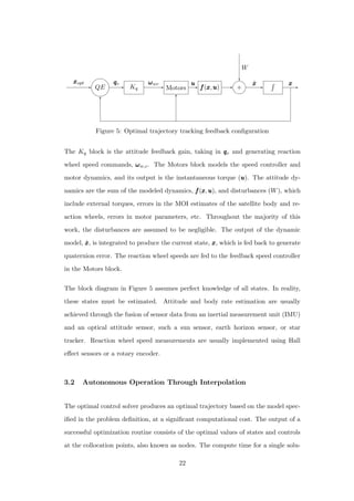
To test this approach, one of the grid points is chosen as the target, but that tra-
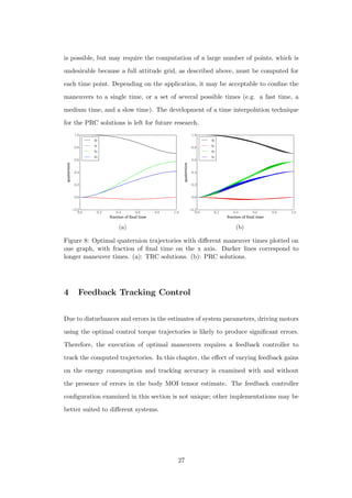
jectory is not included in the interpolation. Figure 6 plots the PSOPT computed
solution for the target point, as well as those of its nearest neighbors to help visualize
why the interpolation works. Figure 7 shows the computed solution compared to the
interpolated solution. The maximum quaternion error does not exceed 0.004. Note
that in Figure 6, the line labeled q0 is actually q0 −1, since two identical quaternions
will produce a quaternion error of [1 0 0 0]T .
24](https://image.slidesharecdn.com/2e1917f8-359f-47e1-92a7-a1899f984d19-160719215916/85/Dmitriy-Rivkin-Thesis-36-320.jpg)
![4.1 Tracking Controller Configuration
The ability to track a given trajectory requires estimation of the current attitude
quaternion and computation of the error. Attitude estimation is beyond the scope
of this work, and the availability of a perfect estimate is assumed. Crassidis [11]
offers a review of attitude estimation methods. The quaternion error is given by Eq.
35.
qqqe = qqq∗
1 ⊗ qqq2 (35)
The vector part of the error quaternion ([q1 q2 q3]) is then multiplied by a constant,
kq, to produce the desired angular momentum vector, expressed in the body frame.
A similar approach is used in [18]. Unlike [18], the RWA in this work has three
reaction wheels with axes of rotation aligned with the axes of the body frame.
Thus, the angular momentum command can be multiplied by another constant,
kh, to produce the reaction wheel speed commands. Because kq and kh are both
constants they can be combined into a single constant, kQ.
Speed control of an electric motor is achieved by controlling the duty cycle of the
switch mode drive electronics. The duty cycle is usually computed using a PID
(Proportional-Integral-Derivative) controller. For the purposes of simulation in this
work, the PID controller and motor dynamics are not modeled. Instead, speed
control is implemented by multiplying wheel speed error (ωωωw,e) by a constant, kω,
and treating the output as the control torque input, uuu, to the dynamic model,
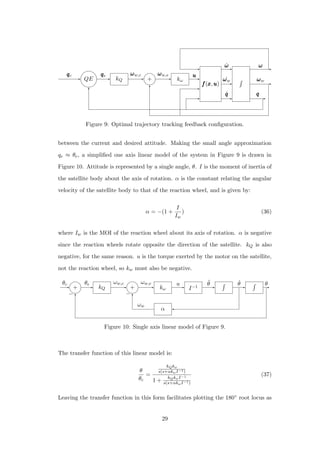
fff(xxx,uuu). Figure 9 summarizes the full feedback control system used in the simulation
of trajectory tracking.
4.2 Single Axis Linear Model
If rotation is constrained to a single axis parallel to one of the axes of the body frame,
then the quaternion error about that axis is sin(θe), where θe is the angular distance
28](https://image.slidesharecdn.com/2e1917f8-359f-47e1-92a7-a1899f984d19-160719215916/85/Dmitriy-Rivkin-Thesis-40-320.jpg)
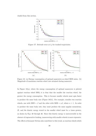
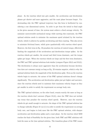
![(see Figure 22), more nodes are required to obtain a solution which is close to the
optimum than for the smooth solutions to the TRC. The greater the number of
nodes, the greater the computational burden. All solutions presented in this work
have 50 nodes, and it is immediately clear upon observation of optimal control
trajectories, such as those in Figures 21 and 22, that the TRC optimal solutions are
significantly less noisy. In short, TRC optimal solutions are less challenging to obtain
and implement. On the other hand, the PRC optimal trajectories always outperform
them with respect to the energy metric of Eq. 25, since the PRC yields solutions that
are optimal with respect to that metric. The amount of performance improvement
obtained using the PRC depends on the attitude control system and the nature of
maneuvers it is executing. For example, as will be shown in the next section, if the
reaction wheels are large, the PRC does not deliver enough improvement over the
TRC to justify the increased complexity of implementation.
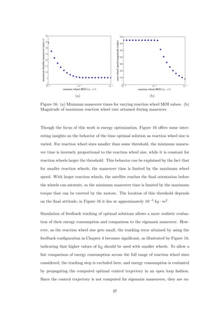
5.1 Varying Reaction Wheel MOI
The reaction wheel MOI values were varied between 10−6 kg · m2 and 10−4 kg · m2
at 21 discreet, logarithmically distributed points, with qf = [0.71 0.00 0.57 0.42] for
all runs. The final time was set to 30s. In order to verify that feasible solutions
existed for each value of reaction wheel MOI, time optimal solutions were computed
(Figure 16). For the smallest reaction wheel size evaluated, MOI = 10−6 kg · m2,
the minimum maneuver time was about 35s, so that point was excluded from energy
optimization. It is worth noting that 10−6 kg · m2 is approximately the MOI of the
motors’ rotors without any extra mass attached.
36](https://image.slidesharecdn.com/2e1917f8-359f-47e1-92a7-a1899f984d19-160719215916/85/Dmitriy-Rivkin-Thesis-48-320.jpg)
![0 5 10 15 20 25 30
time (s)
−0.0015
−0.0010
−0.0005
0.0000
0.0005
0.0010
0.0015
0.0020
0.0025
controltorque(N·m)
u1
u2
u3
(a)
0 5 10 15 20 25 30
time (s)
−0.0015
−0.0010
−0.0005
0.0000
0.0005
0.0010
0.0015
0.0020
0.0025
controltorque(N·m)
u1
u2
u3
(b)
0 5 10 15 20 25 30
time (s)
−0.0015
−0.0010
−0.0005
0.0000
0.0005
0.0010
0.0015
0.0020
0.0025
controltorque(N·m)
u1
u2
u3
(c)
0 5 10 15 20 25 30
time (s)
−0.0015
−0.0010
−0.0005
0.0000
0.0005
0.0010
0.0015
0.0020
0.0025
controltorque(N·m)
u1
u2
u3
(d)
Figure 22: PRC optimal control trajectories for four points in Figure 19. (a) First
point from the left. (b) Sixth point from the left. (c) Sixteenth point from the left.
(d) Twentieth point from the left.
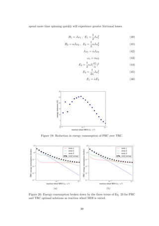
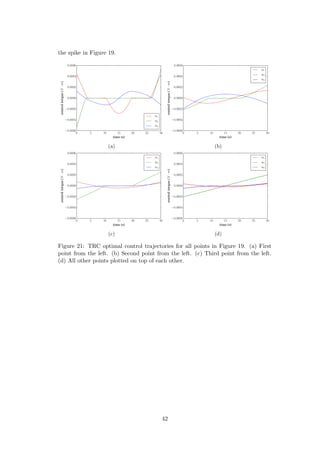
5.2 Varying Maneuver Time
In this section, the reaction wheel MOI is held fixed at 2.2 × 10⁻⁵kg · m2, which is
the MOI of a commercially available Cubesat reaction wheel [2]. The final attitude
of the maneuver is the same as that in used in the previous section. From Figure
16, it is known that the minimum time for this maneuver is approximately 5.5
s. Therefore, the shortest maneuver time examined is 6s, and the longest is 600s.
Energy consumption for 21 values of tf , distributed logarithmically between the two
extremes, is plotted in Figure 23(a). As in the previous section, the feedback tracking
is not simulated, and the eigenaxis trajectory is not included for comparison. The
reaction wheel speeds do not saturate during any of the maneuvers (Figure 23(b)),
which is unsurprising since the reaction wheel MOI is large enough that even the
43](https://image.slidesharecdn.com/2e1917f8-359f-47e1-92a7-a1899f984d19-160719215916/85/Dmitriy-Rivkin-Thesis-55-320.jpg)
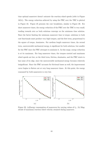
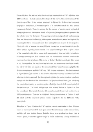
![5.3 Varying Final Attitude
In this section, the maneuver time is held constant at 30s (unless otherwise specified)
and the reaction wheel MOI is set to 2.2 × 10⁻⁵ kg · m2. The final attitude is varied
in two ways: first the axis of rotation is held constant while the magnitude is varied,
and then the axis is varied as the magnitude is held constant.
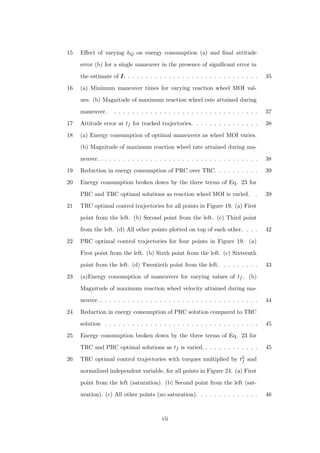
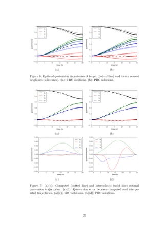
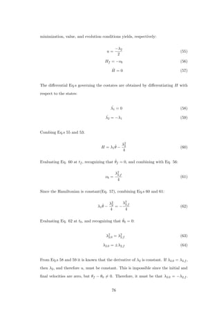
To generate Figure 28, the axis of rotation is set to eee = [0.00 0.81 0.59] and the
maneuver angle (θ) is varied between π
10 and π. The cost breakdown is computed
in the same manner as for Figure 20. As expected, the energy consumption of the
maneuver increases with increasing θ. The first two terms of Eq. 23 dominate, as
the reaction wheel speeds are not high enough to create significant frictional losses.
The percent energy reduction achieved using the PRC over the TRC is plotted in
Figure 29, for three values of tf . The variation in improvement is slight for all tf .
In Figure 25, the dominating term changed as tf was varied, leading to significant
variation in energy reduction. In contrast, as θ is varied, the relative importance of
the terms remains approximately constant, resulting in small variation.
0.5 1.0 1.5 2.0 2.5 3.0
maneuver angle (rad)
−0.05
0.00
0.05
0.10
0.15
0.20
0.25
0.30
TRC:energyconsumption(Joules)
term 1
term 2
term 3
total energy
(a)
0.5 1.0 1.5 2.0 2.5 3.0
maneuver angle (rad)
−0.05
0.00
0.05
0.10
0.15
0.20
0.25
0.30
PRC:energyconsumption(Joules)
term 1
term 2
term 3
total energy
(b)
Figure 28: Energy consumption broken down by the three terms of Eq. 23 for TRC
and PRC optimal solutions as maneuver angle is varied.
48](https://image.slidesharecdn.com/2e1917f8-359f-47e1-92a7-a1899f984d19-160719215916/85/Dmitriy-Rivkin-Thesis-60-320.jpg)
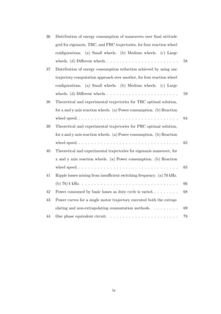
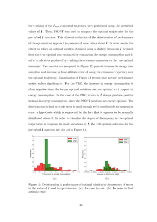
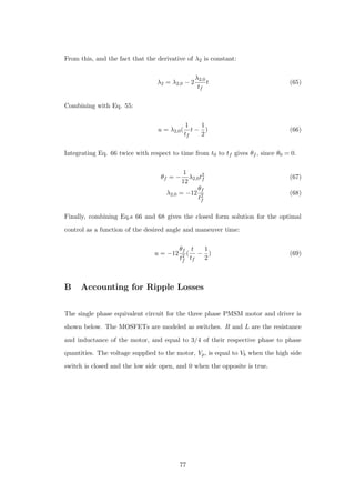
![improvement by using the PRC is significant. The reaction wheel MOI is set to
1 × 10⁻⁴, 1 × 10⁻⁵, and 1 × 10⁻⁵ kg · m2 for the x, y, and z wheels respectively. The
maneuver axis and angle are varied in the same fashion as in the previous section,
because it is expected that the energy reduction will have a strong dependence on
the final attitude.
0.0 0.5 1.0 1.5 2.0 2.5 3.0 3.5
maneuver magnitude (rad)
0
10
20
30
40
50
60
energyreduction(%)
different wheels
small wheels
large wheels
(a)
0.0 0.5 1.0 1.5 2.0 2.5 3.0 3.5
maneuver magnitude (rad)
−0.1
0.0
0.1
0.2
0.3
0.4
0.5
energy(Joules)
different wheels
small wheels
large wheels
(b)
Figure 32: Variation of maneuver angle for three reaction wheel configurations.
Wheel MOI are (in kg · m2 × 10−5): different wheels = [10 1 1], small wheels =
[1 1 1], large wheels = [10 10 10]. (a) Percent energy reduction using PRC over
TRC. (b) Energy consumption of PRC optimal solutions.
In Figure 32(a) energy reduction of PRC over TRC solutions is plotted for three
reaction wheel configurations as θ is varied and the rotation axis is kept constant
at eee = [0.00 0.81 0.59]. The first is the configuration with differing wheel sizes as
described above. The next one is a configuration where all wheels are the same size,
with MOI equal to that of the small wheels in the differing wheel size configuration.
The last one has three uniform wheels with MOI equal to that of the large wheel of
the different wheel size configuration. Notice that the x component of the rotation
axis, which is the axis with the big wheel, is zero. It is observed that for maneuver
angles smaller than π
2 rad, the improvement for different wheels is nearly identical
to that of the uniform small wheels, but above π
2 rad the improvement rises rapidly
and ultimately reaches 50% at θ = π rad. The reason for this radical shift is best
explained by examining the body rate trajectories in Figure 33. In (a) and (b),
where θ = π
2 , the majority of the angular rate is allocated to the y and z axes and
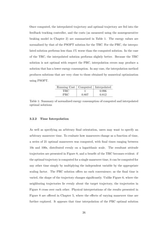
51](https://image.slidesharecdn.com/2e1917f8-359f-47e1-92a7-a1899f984d19-160719215916/85/Dmitriy-Rivkin-Thesis-63-320.jpg)
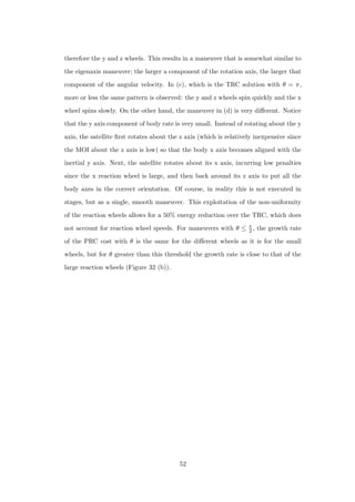
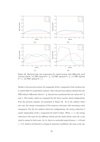
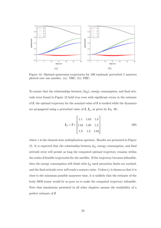
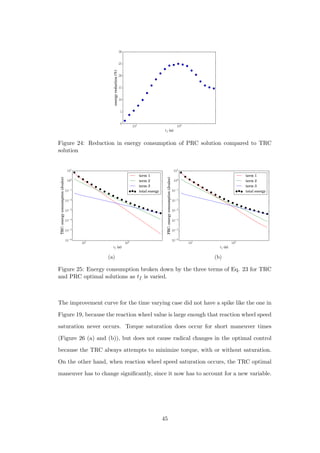
![that occurred when the maneuver angle passed π
2 in Figure 32. This is confirmed
by Figure 35, where PRC optimal body rate trajectories for the points in Figure 32
(c) with z = 0.6 and z = 0.7 are plotted.
−0.2 0.0 0.2 0.4 0.6 0.8 1.0 1.2
z component of rotation axis
−10
0
10
20
30
40
50
60
70
energyreduction(%)
small wheels
large wheels
different wheels
(a)
−0.2 0.0 0.2 0.4 0.6 0.8 1.0 1.2
z component of rotation axis
0.0
0.2
0.4
0.6
0.8
energy(Joules)
small wheels
large wheels
different wheels
(b)
−0.2 0.0 0.2 0.4 0.6 0.8 1.0 1.2
z component of rotation axis
−10
0
10
20
30
40
50
60
70
energyreduction(%)
small wheels
large wheels
different wheels
(c)
−0.2 0.0 0.2 0.4 0.6 0.8 1.0 1.2
z component of rotation axis
0.0
0.2
0.4
0.6
0.8
energy(Joules)
small wheels
large wheels
different wheels
(d)
Figure 34: Variation of z component of rotation axis for three reaction wheel con-
figurations. Wheel MOI are (in kg · m2 × 10−5): different wheels = [10 1 1], small
wheels = [1 1 1 ], large wheels = [10 10 10]. (a) Percent energy reduction of PRC
over TRC solutions, θ = π
2 . (b) Energy consumption of PRC optimal solutions,
θ = π
2 . (c) Percent energy reduction of PRC over TRC solutions, θ = π. (d) Energy
consumption of PRC optimal solutions, θ = π.
54](https://image.slidesharecdn.com/2e1917f8-359f-47e1-92a7-a1899f984d19-160719215916/85/Dmitriy-Rivkin-Thesis-66-320.jpg)
![consumption values are computed by simulating feedback tracking of the computed
trajectories using the feedback controller in Chapter 4. Though the dynamics use a
quaternion attitude representation, the sample points were chosen so as to comprise
a uniform grid in the standard [yaw pitch roll] euler angle attitude representation.
In order to sample the entire space of attitude maneuvers, the yaw, pitch, and roll
ranges are, respectively: [−π, π], [−π
2 , π
2 ], and [−π, π]. These are discretized with a
resolution of π
10, so that there are 21 sample points in yaw, 11 in pitch, and 21 in
roll, resulting in a three dimensional grid of 21 × 11 × 21 = 4851 points. The ma-
neuver time is 30s for all maneuvers presented in this section. Four configurations
of reaction wheels are used, with the following values of MOI about their rotational
axes (in kg · m2 × 10−5): small wheels [1 1 1], medium wheels [2.2 2.2 2.2], large
wheels [10 10 10], and differently sized wheels [10 1 1].
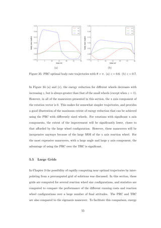
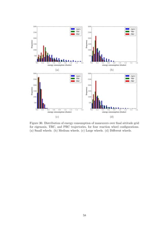
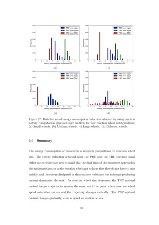
The resulting distributions of energy consumption and energy reduction are pre-
sented in Figures 36 and 37, and summarized in Tables 2 and 3. In the case of
uniform wheel sizes, energy reduction of PRC over TRC remained fairly constant
across all maneuvers, so the averages presented in Table 3 for the uniform wheel size
configuration are quite close to the improvements computed for a single final atti-
tude in Figure 19. Improvements of the PRC and TRC over eigenaxis maneuvers are
more variable. This is explained by fact that the eigenaxis maneuver does not take
into account the dynamics of the satellite, so for some final attitudes the eigenaxis
path happens to be closer to the optimal path than for others. For example, when
the eigenaxis is aligned with the axis of rotation of one of the reaction wheels, the
paths taken by the optimal solutions and eigenaxis solution are likely to be nearly
the same. In this case, the difference between the trajectories would lie only in the
acceleration profile. On the other hand, the paths taken by the TRC and PRC
optimal trajectories always tends to be quite similar, with most of the difference
in energy consumption being accounted for by differing acceleration profiles. This
explains the consistency of improvement of the PRC over the TRC. For the differ-
ently sized wheels, the PRC over TRC energy reduction ranges between about 5 %
and 60 %. The origins of this deviation were discussed in the previous section. The
56](https://image.slidesharecdn.com/2e1917f8-359f-47e1-92a7-a1899f984d19-160719215916/85/Dmitriy-Rivkin-Thesis-68-320.jpg)
![6 Hardware Implementation
The work presented in previous chapters performed optimization based on a power
model which included three loss sources: resistive losses in the motor armature, fric-
tional losses, and mechanical energy which cannot be recaptured when a regenerative
braking system is lacking. The availability of a high performance motor driver with
negligible losses was assumed. In order to evaluate the performance of the optimal
solutions with a real world driver, a BLDC driver board was built. The driver losses
incurred by this board proved to be non-negligible, and, for the evaluated trajectory,
both the TRC and eigenaxis maneuvers outperformed the PRC. For all trajectories,
energy consumption was significantly higher than that which was predicted. In order
to explain this discrepancy, several driver loss sources were evaluated, and the pri-
mary culprit was identified as inaccuracy in the rotor position estimate. Though the
test was not successful, it motivated the evaluation of conditions on the motor driver
that must be met in order for this kind of trajectory optimization to be valuable.
It was also observed that power consumption was proportional to the magnitude of
reaction wheel velocity with a low performance commutation algorithm, suggesting
that trajectory optimization of a running cost equal to the absolute value of the
reaction wheel velocity would be valuable if such an algorithm were used.
6.1 Experimental Set Up
A momentum wheel with a MOI of approximately 1×10⁻⁵kg·m2 was attached to the
rotor of a Faulhaber 2010 012b BLDC motor [3] which was affixed to a tabletop. The
motor was driven using a Texas Instruments DRV8312 integrated brushless motor
driver [33]. Control signals to the driver were generated by a dsPIC33 microcontroller
[25]. The microcontroller uses signals from the motor’s integrated Hall effect sensors
to drive a rotor position and speed estimator and uses these estimates to implement
speed control and commutation. The commutation algorithm used was space vector
modulation (SVM) [24], the only motor quantity measured by the controller being
61](https://image.slidesharecdn.com/2e1917f8-359f-47e1-92a7-a1899f984d19-160719215916/85/Dmitriy-Rivkin-Thesis-73-320.jpg)
![are available. [24] offers an excellent overview of PMSM motor control techniques.
In brief, the goal of PMSM motor control is to generate the appropriate voltages
on each of the motor’s three phases such that the magnetic field produced by the
armature coils is 90◦ electrical ahead of that of the rotor, so as to produce the max-
imum amount of torque for a given current, and eliminate torque ripple. To do so
requires precise knowledge of the orientation of the rotor at all times. Rotary en-
coders are often used to obtain this information. However, the test setup only had
hall effect sensors, not an encoder. Thus, a Kalman filter based on Hall effect sensor
measurements was implemented to estimate the rotor position.
Hall effect sensors provide an absolute position measurement with a resolution of
60◦ electrical. However, the position is known relatively precisely when the Hall
effect sensor state transitions. Velocity is estimated by measuring the time between
Hall effect sensor transitions. With the velocity known, the rotor angle can be
extrapolated from the precisely known transition orientation. Since the dynamics
of the reaction wheel are simple, this approach works relatively well. However,
there is a non-negligible amount of noise in the velocity measurements that can
arise from imperfect placement of Hall effect sensors and delays in transition time
latching. Furthermore, this method produces errors when the motor is accelerating.
Attempts to account for acceleration in the estimator failed to improve performance.
The estimator also performs poorly at low speeds when transitions between Hall
effect sensors are infrequent.
6.3 Speed Control
In order to maintain comparability to the simulation, the speed controller that was
implemented was similar to that described in Chapter 4, where the speed error is
multiplied by a constant to produce the commanded torque. The torque produced
by the motor (τ) can be approximated by:
τ = kt ∗
(Vo − Vm)
R
(48)
63](https://image.slidesharecdn.com/2e1917f8-359f-47e1-92a7-a1899f984d19-160719215916/85/Dmitriy-Rivkin-Thesis-75-320.jpg)
![losses (PHS
switch), is given in [26]:
PHS
switch =
1
2
× Vb × Ib × tR × fsw (49)
PLS
switch =
1
2
× Vb × Ib × tF × fsw (50)
Pswitch = PHS
switch + PLS
switch (51)
where tR and tF are the output rise and fall times, respectively, and fsw is the
switching frequency. The rise and fall times depend on the load. With a resistive
load, these are both quoted as 14ns in the motor driver datasheet [33], though with
an inductive load they may be higher. fsw in the experimental setup is 70 kHz,
so, using the quoted rise and fall times, tR × fsw = tF × fsw = 0.00098, meaning
these losses are negligible. Conduction losses, due to the effective resistance of a
fully turned on switch, are also insignificant, as the MOSFETs’ turned on resistance
(80mΩ) is two orders of magnitude lower than that of the coil windings.
Even when the motor was stationary and no torque is applied (or when the motor was
disconnected), a significant amount of current consumption was observed when the
driver was enabled. These losses, hereafter referred to as basic losses, proved to be
dependent on the switching frequency and the duty cycle, and are likely the result of
the combined effect of gate drive losses, shoot through, and output capacitive losses,
since these are independent of load current [17]. These losses were characterized
by setting the same duty cycle on all three phases so that no current was made to
flow through the motor, and then measuring the current consumed by the driver.
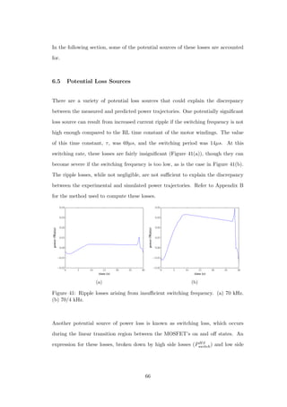
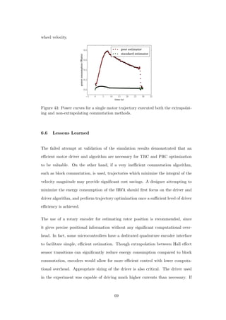
The effects of varying the duty cycle on the basic losses are presented in Figure 42.
Because basic losses drop to zero for both 0% and 100% duty cycles, it is clear that
they are rooted in the switching action of the driver. These losses are significant,
as evident from Figure 42, and are estimated to account for approximately 1/4 of
energy consumption.
We believe that the majority of the added cost of the experimental trajectories stems
from error in the rotor orientation estimate. If the stator field is not optimally
67](https://image.slidesharecdn.com/2e1917f8-359f-47e1-92a7-a1899f984d19-160719215916/85/Dmitriy-Rivkin-Thesis-79-320.jpg)
![8 Appendices
A Derivation of 1D TRC Optimal Solution
The one dimensional equivalent of the dynamics can be formulated as:
˙θ
¨θ
=
0 1
0 0
θ
˙θ
+
0
I−1
u (52)
Where θ is the orientation angle, u is the torque exerted by the control system on the
satellite, and I is the MOI of the satellite body. For the remainder of this derivation,
we set I = 1 for notational simplicity. Since the TRC does not include the reaction
wheel speed, the reaction wheel dynamics needn’t be modeled, and it is assumed
that no state or control saturation limits are reached.
An analytical solution is obtained through the application of Pontryagin’s principle.
Notation is adopted from [29]. First, the Hamiltonian (H) is formulated as:
H = u2
+ λ1
˙θ + λ2u (53)
where λ1 and λ2 are the costates corresponding to θ and ˙θ, respectively. The end-
point constraints are used to formulate the endpoint Lagrangian ( ¯E) as follows:
¯E = ν1(θ0 − 0) + ν2(θf − θf
) + ν3( ˙θ(t0) − 0) + ν4( ˙θf − 0) + ν5(t0 − 0) + ν6(tf − tf
)
(54)
where a subscript of 0 or f indicates the initial or final value of a variable, a super-
script indicates the initial or final value of a variable required by a constraint, and
ν1 through ν6 are endpoint Lagrange multipliers. Application of the Hamiltonian
75](https://image.slidesharecdn.com/2e1917f8-359f-47e1-92a7-a1899f984d19-160719215916/85/Dmitriy-Rivkin-Thesis-87-320.jpg)
![Vb
R L
+
−Vm
i
Figure 44: One phase equivalent circuit.
Circuit analysis gives the following first order differential Eq. for the current, i:
di
dt
+
R
L
= k (70)
k =
2
3
Vp − Vm
R
(71)
the solution to which is:
i = k(1 − e−t/τ
) + i0e−t/τ
(72)
τ =
L
R
(73)
where i0 is the current at t = 0. The energy dissipated by the resistance between
t = 0 and t = tf is:
tf
0
Ri2
dt = k2
[tf + 2τ(e−tf /τ
− 1) +
τ
2
(1 − e−2tf /τ
)]+
ki0τ[2(1 − e−tf /τ
) + e−2tf /τ
− 1]+
i2
0
τ
2
[1 − e−2tf /τ
] (74)
assuming that k is constant. Given i0, the switching period (tp), the duty cycle
(d), Vb, and Vm, Eq. 74 can be used to evaluate the energy consumed by a single
switching cycle. Dividing this energy by the switching period yields the average
power consumption during the cycle. Since the switching rate is much higher than
78](https://image.slidesharecdn.com/2e1917f8-359f-47e1-92a7-a1899f984d19-160719215916/85/Dmitriy-Rivkin-Thesis-90-320.jpg)
![the mechanical time constant of the rotor, Vm is assumed to be constant, therefore
the assumption that k is constant is satisfied, provided that the high and low phases
of the switching cycle are analyzed separately.
Vm is obtained by multiplying the rotor speed by the motor’s electrical constant. The
average current during a switching cycle, iavg, is obtained by dividing the control
torque by the torque constant. d and i0 are then chosen such that i0 = if (the
current at the end of the switching cycle) and the average current during the cycle
is equal to iavg.
Having solved for the total power dissipated in the resistance, the ripple current
losses are found by subtracting power consumption computed with some very small
value of tp from the total power consumption.
References
[1] HSL. A collection of Fortran codes for large scale scientific computation.
http://www.hsl.rl.ac.uk.
[2] Micro Reaction Wheel. Technical report, Blue Canyon Technologies, Boulder,
Colorado.
[3] Series 2610 ... B Datasheet. Technical report, Dr. Fritz Faulhaber GMBH &
CO. KG, 2014.
[4] P.R. Amestoy, I.S. Duff, J. Koster, and J.-Y. L’Excellent. A fully asynchronous
multifrontal solver using distributed dynamic scheduling. SIAM Journal of
Matrix Analysis and Applications, 23(1):15–41, 2001.
[5] V.M. Becerra. PSOPT Optimal Control Solver User Manual. Release 3, 2010.
Available: http://code.google.com/p/psopt/downloads/list”.
79](https://image.slidesharecdn.com/2e1917f8-359f-47e1-92a7-a1899f984d19-160719215916/85/Dmitriy-Rivkin-Thesis-91-320.jpg)
![[6] Nazareth S. Bedrossian, Sagar Bhatt, Wei Kang, and I. Michael Ross. Zero-
propellant maneuver guidance. IEEE Control Systems Magazine, 29(5):53–73,
2009.
[7] J.T. Betts. Practical Methods for Optimal Control and Estimation Using Non-
linear Programming. Society for Industrial and Applied Mathematics, 2010.
[8] K.D. Bilimoria and B. Wei. Time-optimal three-axis reorientation of rigid space-
craft. Journal of Guidance, Control, and Dynamics, 16(3):446–452, 1993.
[9] Robin Blenden and Hanspeter Schaub. Regenerative Power-Optimal Reac-
tion Wheel Attitude Control. Journal of Guidance, Control, and Dynamics,
35(4):1208–1217, 2012.
[10] Cal Poly SLO. Cubesat Design Specification (Rev 13), 2015.
[11] John L Crassidis, F. Landis Markley, and Yang Cheng. A Survey of Nonlinear
Attitude Estimation Methods. Journal of Guidance, Control, and Dynamics,
30:12–28, 2007.
[12] Michael James Develle. Optimal Attitude Control Management For A Cubesat.
Master’s thesis, University of Central Florida, 2011.
[13] Andrew Fleming. Real-Time Optimal Slew Maneuver Design and control. Mas-
ter’s thesis, Naval Postgraduate School, 2004.
[14] Andrew Fleming, Pooya Sekhavat, and I Michael Ross. On The Minimum-Time
Reorientation of a Rigid Body. In AIAA Guidance, Navigation, and Control
Conference, Chicago, IL, 2009.
[15] E. Gill, P. Sundaramoorthy, J. Bouwmeester, B. Zandbergen, and R. Reinhard.
Formation flying within a constellation of nano-satellites: The QB50 mission.
Acta Astronautica, 82(1):110–117, 2013.
[16] Qi Gong, Fariba Fahroo, and I. Michael Ross. Spectral Algorithm for Pseu-
dospectral Methods in Optimal Control. Journal of Guidance, Control, and
Dynamics, 31(3):460–471, 2008.
80](https://image.slidesharecdn.com/2e1917f8-359f-47e1-92a7-a1899f984d19-160719215916/85/Dmitriy-Rivkin-Thesis-92-320.jpg)
![[17] David Jauregui, Bo Wang, and Rengang Chen. Power Loss Calculation with
Common Source Inductance consideration for Synchronous Buck Converters.
SLPA009-20011 Texas Instruments . . . , (July):17, 2011.
[18] Mark Karpenko, Sagar Bhatt, Nazareth Bedrossian, and I. Michael Ross. Flight
Implementation of Shortest-Time Maneuvers for Imaging Satellites. Journal of
Guidance, Control, and Dynamics, 37(4):1069–1079, 2014.
[19] Siddharth S Kedare. Space Environment Modelling and Torque-Optimal Guid-
ance for CubeSat Applications. Master’s thesis, Carleton University, 2014.
[20] Planet Labs. Planet Labs Home Page, 2016.
[21] Unsik Lee and Mehran Mesbahi. Quaternion Based Optimal Spacecraft Reori-
entation. Advances in the Astronautical Sciences, 150:1–16, 2014.
[22] Harleigh Marsh, Qi Gong, and Mark Karpenko. Minimum energy attitude
control. Technical report, Naval Postgraduate School, 2015.
[23] Robert G. Melton. Hybrid methods for determining time-optimal, constrained
spacecraft reorientation maneuvers. Acta Astronautica, 94(1):294–301, 2014.
[24] James Robert Mevey. Sensorless Field Oriented Control of Brushless Perma-
nent Magnet Synchronous Motors. PhD thesis, Kansas State University, 2006.
[25] Microchip Technology. dsPIC33EPXXXGP50X, dsPIC33EPXXXMC20X/50X
and PIC24EPXXXGP/MC20X - 16-Bit Microcontrollers and Digital Signal
Controllers with High-Speed PWM, Op Amps and Advanced Analog, 2013.
[26] Peter Millett. SLVA504 Calculating Motor Driver Power Dissipation.
(February):1–5, 2012.
[27] I Michael Ross and Fariba Fahroo. Legendre pseudospectral approximations of
optimal control problems. New Trends in Nonlinear Dynamics and Control and
their Applications, 295(January):327–342, 2003.
[28] I. Michael Ross and Mark Karpenko. A review of pseudospectral optimal con-
trol: From theory to flight. Annual Reviews in Control, 36(2):182–197, 2012.
81](https://image.slidesharecdn.com/2e1917f8-359f-47e1-92a7-a1899f984d19-160719215916/85/Dmitriy-Rivkin-Thesis-93-320.jpg)
![[29] I.M. Ross. A Primer on Pontryagin’s Principle in Optimal Control. Collegiate
Publishers, 2 edition, 2015.
[30] Hanspeter Schaub. AIAA 2008-6259 Locally Power-Optimal Spacecraft Atti-
tude Control for Redundant Reaction Wheel Cluster. In AIAA/AAS Astrody-
namics Specialist Conference, Honolulu, Hawaii, 2008.
[31] Haijun Shen and Panagiotis Tsiotras. Time-Optimal Control of Axi-Symmetric
Rigid Spacecraft. In AIAA Guidance, Navigation, and Control Conference,
Boston, MA, 1998.
[32] Planetary Society. Planetary Society Web Page.
[33] Texas Instruments. DRV83x2 Three-Phase PWM Motor Driver, 2014.
[34] Andreas W¨achter and Lorenz T. Biegler. On the implementation of primal-dual
interior point filter line-search algorithm for large-scale nonlinear programming.
Mathematical Programming, 106:25–57, 2006.
[35] A. Walther and A. Griewant. Getting started with adol-c. In U. Naumann
and O.Schenk, editors, Combinatorial Scientific Computing, pages 181–202.
Chapman-Hall CRC Computational Science, 2012.
[36] Bradley Watanabe. A Small Scale Reaction Wheel Prototype for Attittude Sta-
bilization of Cubesats. Master’s, University of California Santa Cruz, 2013.
[37] E.W. Weisstein. ”Legendre Polynomial.” From MathWorld–A Wolfram Web
Resource. http://mathworld.wolfram.com/LegendrePolynomial.html.
[38] Bong Wie. Space Vehicle Dynamics And Control. American Institute of Aero-
nautics and Astronautics, Reston, Virginia, 2 edition, 2008.
[39] Rafal Wisniewski and Piotr Kulczycki. Slew Maneuver Control for Spacecraft
Equipped with Star Camera and Reaction Wheels. Control Engineering Prac-
tice, 13(3):349–356, 2005.
82](https://image.slidesharecdn.com/2e1917f8-359f-47e1-92a7-a1899f984d19-160719215916/85/Dmitriy-Rivkin-Thesis-94-320.jpg)