This dissertation proposes a model-based control approach for a reconfigurable robot. The author first develops a methodology to model the kinematics of a reconfigurable robot with variable Denavit-Hartenberg parameters, allowing it to take on different open kinematic structures. Advanced model-based linear and nonlinear control strategies are then employed to control the robot, including mixed sensitivity H-infinity control, H-infinity control, mu-synthesis control, linear parameter varying control, feedback linearization control, sliding mode control, and adaptive control. Simulation results demonstrate the effectiveness of these control approaches. The author also develops an algorithm to select the optimal kinematic structure and control method for a given geometric task to maximize tracking performance.

![List of Figures
1.1 Definition of standard Denavit and Hartenberg (D–H) parameters.
Source; Manseur, [63]............................................................................ 2
1.2 Set of design variables of the 3-DOF configuration modular robots,
this set is a commercial product of AMTEC GmbH Company. Source;
I.M. Chen, [22]...................................................................................... 4
1.3 Mechanical set up of a modular and reconfigurable robot (left). The
ICT power cube Mechatronical component (right). Source; Strasser,
[84]........................................................................................................ 5
1.4 Robotic system with motion control system, inner and outer loop
controllers.............................................................................................. 6
1.5 Standard robust control problem. ......................................................... 9
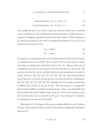
2.1 Kinematic structures of the ABB and Stanford robots, D–H param-
eters are from sources; Dawson, [57] and Spong, [80]........................... 15
2.2 The spherical wrist, joint axes 4, 5 and 6. ............................................ 16
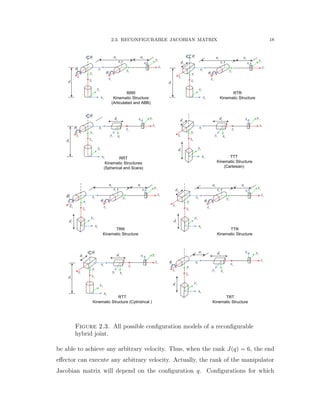
2.3 All possible configuration models of a reconfigurable hybrid joint........ 18
2.4 Workspace of RRR Configuration with four different twist angle val-
ues π{16, π{8, π{4, and π{2. ................................................................. 21
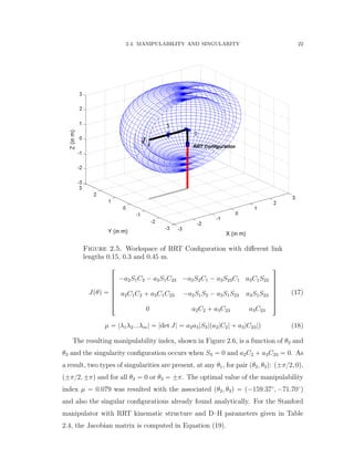
2.5 Workspace of RRT Configuration with different link lengths 0.15, 0.3
and 0.45 m. ........................................................................................... 22
2.6 3D profile of the manipulability index measure of RRR configuration. 23
2.7 3D profile of the manipulability index measure of RRT configuration.. 24
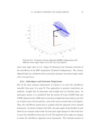
2.8 Cartesian velocity ellipsoid of RRR configuration with different twist
angle values of pπ{16, π{6, π{2q degrees................................................. 26
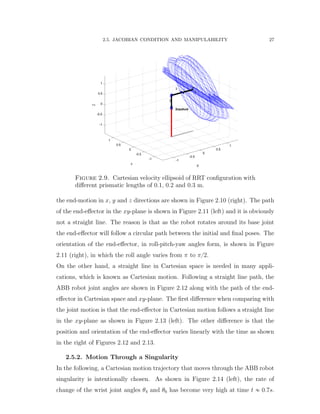
2.9 Cartesian velocity ellipsoid of RRT configuration with different pris-
matic lengths of 0.1, 0.2 and 0.3 m. ...................................................... 27
x](https://image.slidesharecdn.com/06f80bb7-ba1f-45e9-aa53-783373e47302-151229194001/85/Final-10-320.jpg)
![List of Tables
2.1 D–H parameters of the n-GKM model.................................................. 12
2.2 D–H of a spherical wrist, source; Spong, [80]. ...................................... 17
2.3 D–H parameters of the ABB manipulator robot, source; Spong, [80]. . 21
2.4 D–H parameters of the Stanford manipulator robot, source; Spong,
[80]........................................................................................................ 23
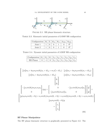
3.1 Reconfiguration parameters values........................................................ 37
3.2 Reconfigurable D–H parameters of the 3-GKM model.......................... 39
3.3 Kinematic initial parameters of 2-DOF RR configuration .................... 40
3.4 Dynamic initial parameters of 2-DOF RR configuration ...................... 40
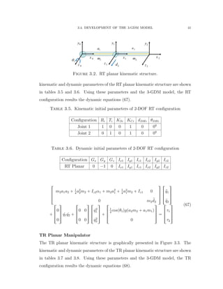
3.5 Kinematic initial parameters of 2-DOF RT configuration..................... 41
3.6 Dynamic initial parameters of 2-DOF RT configuration....................... 41
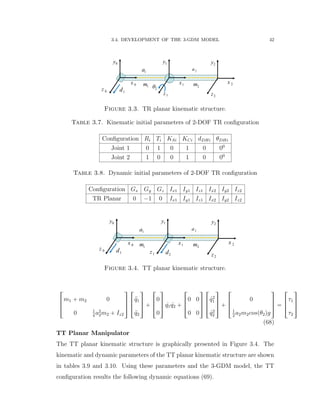
3.7 Kinematic initial parameters of 2-DOF TR configuration .................... 42
3.8 Dynamic initial parameters of 2-DOF TR configuration ...................... 42
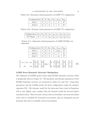
3.9 Kinematic initial parameters of 2-DOF TT configuration .................... 43
3.10 Dynamic initial parameters of 2-DOF TT configuration....................... 43
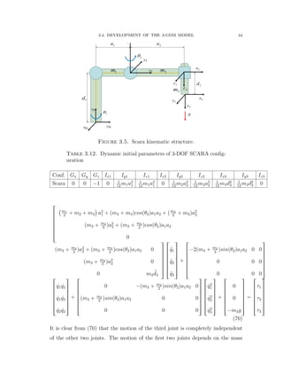
3.11 Kinematic initial parameters of 3-DOF SCARA configuration............. 43
3.12 Dynamic initial parameters of 3-DOF SCARA configuration ............... 44
3.13 D–H parameters of the PUMA 560 Manipulator, source; Fu, [41]........ 46
6.1 Dynamic parameter properties of a reconfigurable robot...................... 136
A.1 Nominal parameter values of the Bosch Scara robot arm ..................... 166
A.2 Nominal parameter values of the Bosch Scara robot arm ..................... 166
A.3 Different values for inertias and damping for different joint position
of link 2 (left). Estimated parameter values for stiction and Coulomb
friction (right). ...................................................................................... 167
xvii](https://image.slidesharecdn.com/06f80bb7-ba1f-45e9-aa53-783373e47302-151229194001/85/Final-17-320.jpg)
![NOMENCLATURE xix
θmi Position of motor axis of joint i rrads
θi Position of joint axis i rrads
9θmi Velocity of motor axis of joint i rrad{ss
9θi Velocity of joint axis i rrad{ss
:θi Acceleration of joint axis i rrad{s2
s
C1 Cospθ1q
S1 Sinpθ1q
C12 Cospθ1 ` θ2q
S12 Sinspθ1 ` θ2q
N1 Gear ratio r1s
τLD,i Disturbance torques on joint i rN ms
δADi Quantization error of sensor joint i rrads
δDA Resolution of DA-converter rV s
δF Perturbation in friction rN ms{rads
δ1{J Perturbation in inertia r1{kgm2
s
δθ Tracking error rrad{ss
p1 Interconnection output to inertia error rN ms
p2 Interconnection output to friction error rrad{ss
q1 Interconnection input to inertia error rN{kgms
q2 Interconnection input to friction error rN ms
US Input voltage to Servo motor [V ]
USA Input voltage to Tacho controller of Amplifier System rV s
ISA Input current to Current controller of Amplifier System rAs
h Sample time [s]
W∆ Scaling function for perturbation matrix](https://image.slidesharecdn.com/06f80bb7-ba1f-45e9-aa53-783373e47302-151229194001/85/Final-19-320.jpg)
![CHAPTER 1
Introduction and Preliminaries
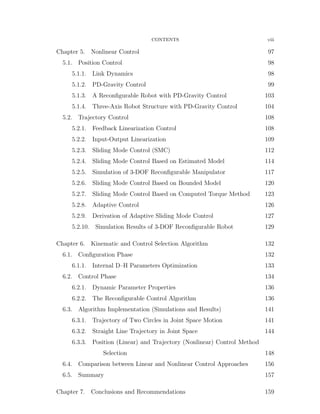
1.1. Introduction to Robot Kinematics
A serial-link manipulator comprises a set of bodies called links connected in a
chain by joints. Each joint has one degree of freedom, either translational (sliding
or prismatic joint) or rotational (revolute joint). To describe the rotational and
translational relationships between adjacent links, Denavit and Hartenberg pro-
posed a matrix method of systematically establishing a coordinate frame to each
link of an articulated chain. The Denavit-Hartenberg (D–H) representation [35]
results a 4ˆ4 homogeneous transformation matrix representing each link’s coordi-
nate frame at the joint with respect to the previous link’s coordinate frame. To
analyze the motion of robot manipulator, coordinate frames are attached to each
link starting from frame F0, attached to the base of the manipulator link, all the
way to the frame Fn, attached to the robot end-effector as shown in Figure 1.1.
Every coordinate frame is determined and established on the basis of three rules:
(1) The zi´1 axis lie along the axis of motion of the ith joint.
(2) The xi axis is normal to the zi´1 axis.
(3) The yi axis completes the right-handed coordinate system as required.
As the frames have been attached to the links, the following definitions of the
link (D–H) parameters are valid:
‚ Joint angle θi is the angle around zi´1 that the common perpendicular
makes with vector xi´1.
‚ Link offset di is the distance along axis zi´1 to the point where the common
perpendicular to axis zi is located.
‚ Link length ai is the length of the common perpendicular to axes zi´1 and
zi.
‚ Link twist αi is the angle around xi that vector zi makes with vector zi´1.
1](https://image.slidesharecdn.com/06f80bb7-ba1f-45e9-aa53-783373e47302-151229194001/85/Final-21-320.jpg)
![1.2. INTRODUCTION TO RECONFIGURABILITY THEORY 2
Figure 1.1. Definition of standard Denavit and Hartenberg (D–H)
parameters. Source; Manseur, [63].
For a rotary joint, di, ai, and αi are the joint parameters and remain constant
for a robot, while θi is the joint variable that changes when link i rotates with
respect to link i ´ 1. For a prismatic joint, θi, ai, and αi are the joint parameters
and remain constant for a robot, while di is the joint variable.
1.2. Introduction to Reconfigurability Theory
Robotics technology has been recently exploited in a variety of areas and var-
ious robots have been developed to accomplish sophisticated tasks in different
fields and applications such as in space exploration, future manufacturing sys-
tems, medical technology, etc. In space, robots are expected to complete different
tasks, such as capturing a target, constructing a large structure and autonomously
maintaining in-orbit systems. In these missions, one fundamental task with the
robot would be the tracking of changing paths, the grasping and the positioning
of a target in Cartesian space. To satisfy such varying environments, a robot with
changeable configuration (kinematic structure) is necessary to cope with these
requirements and tasks. Another field of technology is the new manufacturing en-
vironment, which is characterized by frequent and unpredictable market changes.
A manufacturing paradigm called Reconfigurable Manufacturing Systems (RMS)
was introduced to address the new production challenges [52]. RMS is designed
for rapid adjustments of production capacity and functionality in response to new](https://image.slidesharecdn.com/06f80bb7-ba1f-45e9-aa53-783373e47302-151229194001/85/Final-22-320.jpg)
![1.2. INTRODUCTION TO RECONFIGURABILITY THEORY 3
circumstances, by rearrangement or change of its components and machines. Such
new systems provide exactly the capacity and functionality that is needed, when
it is needed [39]. The rapid changes and adjustments of the RMS structure must
happen in a relatively short time ranging between minutes and hours and not days
or weeks. These systems’ reconfigurability calls for their components, such as ma-
chines and robots to be rapidly and efficiently modifiable to varying demands [48].
Robot manipulators working in extreme or hazardous environments (biological,
chemical, nuclear,..., etc.) often need to change their configuration and kinematic
structures to meet the demands of specific tasks. It is desirable and cost effective
to employ a single versatile robot capable of performing tasks such inspection,
contact operations, assembly (insertion or removal parts), and carrying objects
(pick and place). Robots with maximum manipulability are well conditioned for
dexterous contact tasks [16, 61] and configurations that maximize the robot links
and distance from the environment are suitable for payload handling [56]. The
optimization of a robot workspace over its link lengths, as the design parameters,
is reported in [55, 47], while optimization of kinematic parameters and criteria
for fault tolerance are discussed in [50].
In the literature, modular robotic structures are presented as a solution to cope
with reconfigurable structure of robots. A modular reconfigurable robot consists
of a collection of individual link and joint components that can be arbitrarily as-
sembled into a number of different geometries. Such a system can provide agility
to the user to cope with a wide spectrum of tasks through proper selection and
reconfiguration of a large inventory of functional components. Several prototyping
systems have been demonstrated in various research institutions, [87], [42], [67]
and [13]. An automated generation of D–H parameters methodology has devel-
oped for the modular manipulators [22]. The authors derived the kinematic and
dynamic models of reconfigurable robots using D–H parameters for different sets of
joints, links and gripper modules as shown in Figure 1.2. Furthermore, a library of
modules is formed from which any module can be called with its associated kine-
matic and dynamic models. In [58], a modular and reconfigurable robot design
is introduced with modular joints and links. The proposed design introduces zero](https://image.slidesharecdn.com/06f80bb7-ba1f-45e9-aa53-783373e47302-151229194001/85/Final-23-320.jpg)
![1.2. INTRODUCTION TO RECONFIGURABILITY THEORY 4
Figure 1.2. Set of design variables of the 3-DOF configuration
modular robots, this set is a commercial product of AMTEC GmbH
Company. Source; I.M. Chen, [22].
link offsets to increase the robot’s dexterity and maximize its reachability. A mod-
ular and reconfigurable robot (MRR) with multiple working modes was designed
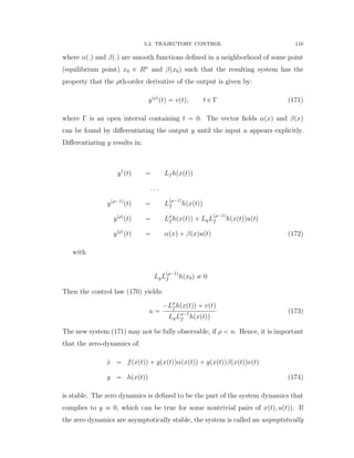
[59]. In the proposed MRR design, each joint module can independently work
in active modes with position or torque control, or passive modes with friction
compensation. With the MRR, the joint module was designed as a hybrid joint
in working modes and not in the sense of mechanical motion. A reconfigurable
robot was proposed [5] and achieves the reconfigurability by utilizing passive and
active joints. In [21], an automated approach was presented to build kinematic
and dynamic models for assembled modular components of robots. The developed
method is applicable to any robotic configuration with a serial, parallel or hybrid
structure. Reconfigurable plug and play robot kinematic and dynamic modeling
algorithms are developed [22]. These algorithms are the basis for the control and
simulation of reconfigurable modular robots. The reconfigurable robot (RRS) was
regarded as a modular system [20]. A task-based configuration optimization based
on a generic algorithm was used to solve a predefined set of joint modules for spe-
cific kinematic configuration. A modular and reconfigurable robot for industrial](https://image.slidesharecdn.com/06f80bb7-ba1f-45e9-aa53-783373e47302-151229194001/85/Final-24-320.jpg)
![1.3. ROBOT CONTROL 5
Figure 1.3. Mechanical set up of a modular and reconfigurable
robot (left). The ICT power cube Mechatronical component (right).
Source; Strasser, [84].
purposes has been introduced [84]. The PROFACTOR GmbH has presented a
modular and reconfigurable robot with power cube (Mechatronical Components)
modules depicted in Figure 1.3. These modules were designed to be identical and
self-contained with actuation, memory, and mechanical, electrical and embedded
programming. A reconfigurable robot has been introduced by [36] that unifies the
kinematic structure of industrial robots. In that unification process, eight mod-
ules were reconfigured by changing configuration parameters. These parameters
represent the trigonometric functions of the robot twist angles.
The main drawbacks of the modular robots proposed in the literature are the
high initial investment necessary in modules that remain idle during many activi-
ties, and the significant lead time for replacement, attachment and detachment of
the components prior to performing a specific task.
1.3. Robot Control
The use of advanced robot control laws may contribute significantly to improve
the robot functions and properties. The improvement of the robot design itself
can also contribute substantially to the desired increase in performance and capa-
bilities. The combination of the controller with proper sensors can provide some](https://image.slidesharecdn.com/06f80bb7-ba1f-45e9-aa53-783373e47302-151229194001/85/Final-25-320.jpg)
![1.3. ROBOT CONTROL 6
sense and awareness of the environment, and improve its accuracy and speed as
well.
Robotic
Arm
Actuator
DC Motor
Outer Loop
Controllers
PD, PID
/H
,q q
, ,d d dq q q
Trajectory
Generation
,q qu
Robotic SystemMotion Control System
Host
Inner Loop
Feedback
Linearization
Controller
Figure 1.4. Robotic system with motion control system, inner and
outer loop controllers.
The former and current problems in the robotics application fields has affected
the research of robot control in a number of fundamental topics: modeling, position
control, robust control and motion planning. This has motives research in robot
modeling, simulation and control design. Therefore, position and trajectory control
is an important research field in robotics control. The position/motion control
problem has received a great deal of interest in robotics. Therefore, a survey that
covers the important control strategies is given with examples and applications.
PD and PID Control
The PD (Proportional-Derivative) and PID (Proportional-Derivative-Integral) con-
trollers are the most applied in industry, which is also true for robotics. Some
references propose a high gain PD controller to ensure global stabilization of the
robot [68, 69, 71], which is unsuited for practical applications due to excitation
of unavoidable higher dynamics and excessive noise amplification. PID controllers
are more suitable to eliminate the steady state error of the final position response.
These controllers introduce an integration action to the resulting closed loop im-
proving the performance tracking requirements.
Feedback Linearization Control
The application of feedback linearization theory to solve robotics control prob-
lems has led to the computed torque approach. Feedback linearization control](https://image.slidesharecdn.com/06f80bb7-ba1f-45e9-aa53-783373e47302-151229194001/85/Final-26-320.jpg)
![1.3. ROBOT CONTROL 7
methods are inner-outer loop control methods: the inner loop must linearize the
plant, whereas the outer loop must achieve the desired closed loop requirements.
Figure 1.4 shows the control motion structure (inner and outer control loops) of a
robot driven by a DC motor. The term Computed Torque Control (CTC) is the
application of PD control at the outer loop to a linearized system by the feedback
linearization control. In robotics, CTC is used to apply PD controllers at the outer
loop independently (every joint controlled separately) [53]. There are two impor-
tant features of the feedback linearization method that require attention: model
error and the outer loop controller design. Feedback linearization is based on the
exact model of the system. Therefore, the controller may be sensitive to modeling
errors such as parameter errors and unmodeled dynamics. Parameter uncertainty
is commonly addressed by either robust control methods or by the derivation of
adaptive controllers [66, 77]. In particular, when a restricted amount of parame-
ters must be estimated (in case of an unknown load), adaptive controllers can be a
suitable approach. The feedback linearization control actively linearized the plant,
such that the resulting system can be considered as a linear system. Therefore,
it is possible to apply one of many linear control methods to close the loop and
achieve the required performance. As a result, a large number of controllers for
the outer loop control are proposed: the standard PD loop of CTC, linear optimal
control [83, 78], sliding mode control, and H8{µ robust optimal controllers.
Lyapunov Based Control
An important tool for control of rigid body systems is Lyapunov stability theory,
which based on the strict dissipation of a suitable energy function [76]. Although
this theory is not constructive to design a controller, a simple structure of the equa-
tions of motion with some relevant assumptions allow a derivation of stabilizing
controllers. These assumptions may include bounded disturbances and bounded
parameter variations. The passivity based control approach attempts to reshape
the robot energy function, rather than imposing a completely different behavior
as with the CTC approach [14, 19]. Experiments have shown and indicated the](https://image.slidesharecdn.com/06f80bb7-ba1f-45e9-aa53-783373e47302-151229194001/85/Final-27-320.jpg)
![1.3. ROBOT CONTROL 8
passivity controllers are more robust than CTC. Another result of Lyapunov sta-
bility theory is the sliding mode control (SMC), which is considered to be a robust
control approach.
Robust Control
To ensure a suitable behavior of the closed loop robot, even in the presence of
modeling errors and disturbances, it is desired to design controllers that are ro-
bust with respect to these errors and disturbances. Modeling errors are generally
separated into parameter errors and unmodeled dynamics, which may have differ-
ent affect on the closed loop system. The standard control framework, adopted in
many textbooks on modern control [23, 60, 88], is shown in Figure 1.5. A con-
troller Kpsq is provided with measurement signals y and has to stabilize a plant
Ppsq with input signals u such that the cost variables z are minimal in some sense,
despite the disturbance signals w and the parametric and dynamic uncertainties
represented in ∆psq. The plant Ppsq is often called the generalized plant or stan-
dard plant since it usually does not only consist of the plant to be controlled, but
can also contain weightings, e.g., parametric and dynamic uncertainty weighting,
input signal thresholds, and the robot dynamic model to be simulated. Also the
other entities can be viewed in a generalized way, e.g., reference signals can be
incorporated as disturbances w and additional feedback paths can be taken in
case of a robust control problem to describe a set of systems, i.e., uncertainty.
A survey can be found covering a number of robust robot position controller de-
sign methods: passivity control, sliding mode control and linear robust control by
factorization approach in [82]. The most popular robust control design method
in robotics literature is the sliding mode control (SMC), also known as Variable
Structure Switching (VSS) control. Sliding mode control is commonly used to ad-
dress parameter uncertainty and bounded disturbances [76, 86]. As mentioned,
SMC is based on upon Lyapunov stability theory, and basically tries to determine
the nominal feedback control law and a corrective control action that steers the
controlled system to the desired behavior, defined as the ‘sliding surface’.](https://image.slidesharecdn.com/06f80bb7-ba1f-45e9-aa53-783373e47302-151229194001/85/Final-28-320.jpg)
![1.3. ROBOT CONTROL 9
yu
w z
( )K s
( )P s
( )s
yu
Figure 1.5. Standard robust control problem.
Optimal Control
Apart from the application of linear outer loop control applied to the feedback
linearized robot, there have been some attempts made to apply optimal control
directly to the rigid body dynamics. The main problem with these approaches
is the amount of assumptions and choices that have to be made to allow for a
solution. For example in [30], an optimal quadratic control is considered with a
special choice optimization criterion, which results in a nonlinear PID controller.
Another example in [44], where an H8-optimal control problem is considered,
results in a nonlinear static state feedback PD controller. Following these methods
to construct a nonlinear controller does not allow the versatility required for a
controller design method needed to solve real-world problems.
The reason is that currently the nonlinear control theory cannot provide a
general robust controller design methodology, due to high complexity of both the
robot model and the involved design specifications. General cases addressed with
optimal control infrequently allow a closed solution, and one has to resort to com-
putationally intensive numerical methods. In the case of special properties of the
uncertainty, e.g., signal roundedness, there do exist applicable controller design
methods, e.g., sliding mode control. These control methods have restricted appli-
cabilities as they cannot exploit structural knowledge of the uncertainty. Linear
control theory does have that capability e.g. H8{µ controller design methods have
limited means of specifying the desired properties of the closed loop system. Linear
control theory also has its limits, but offers a larger variety of specifications.](https://image.slidesharecdn.com/06f80bb7-ba1f-45e9-aa53-783373e47302-151229194001/85/Final-29-320.jpg)
![CHAPTER 2
Development of a Reconfigurable Robot Kinematics
A development of the general n-DOF Global Kinematic Model (n-GKM) is
necessary for supporting any open kinematic robotic arm, and possible redundant
kinematic structures that are intended to support more than 6-DOF. The n-GKM
model is generated by the D–H parameters, given in Table 2.1 and as proposed by
Djuric, Al Saidi, and ElMaraghy [37]. All D–H parameters presented in the Table
2.1 are not fixed values; they are modeled as variables to satisfy the properties of
all possible open kinematic structures of a robotic arm. The twist angle variable
αi is limited to five different values, (00
, ˘900
, ˘1800
), to maintain perpendicular-
ity between joints’ coordinate frames. Consequently, each joint has six different
positive directions of rotations and/or translations.
Table 2.1. D–H parameters of the n-GKM model.
i di θi ai αi
1 R1dDH1 ` T1d1 R1θ1 ` T1θDH1 a1 00
, ˘1800
, ˘900
2 R2dDH2 ` T2d2 R2θ2 ` T2θDH2 a2 00
, ˘1800
, ˘900
. . . . . . . . . . . . . . .
3 RndDHn ` Tndn Rnθn ` TnθDHn an 00
, ˘1800
, ˘900
The subscript DHn implies that the di or θi parameter is constant.
2.1. Modeling of a Reconfigurable Joint
The reconfigurable joint is a hybrid joint that can be configured to be a revolute
or a prismatic type of motion, according to the required task. For the n-GKM
model, a given joint’s vector zi´1 can be placed in the positive or negative directions
of the x, y, and z axis in the Cartesian coordinate frame. This is expressed in
Equations (1)-(2):
12](https://image.slidesharecdn.com/06f80bb7-ba1f-45e9-aa53-783373e47302-151229194001/85/Final-32-320.jpg)
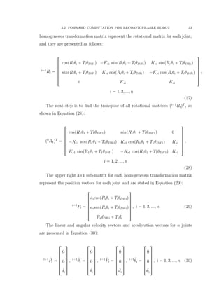
![2.2. MODELING OF RECONFIGURABLE OPEN KINEMATIC ROBOTS 15
N-DOF Reconfigurable Kinematic
Model (RKM) with
Variable D-H Parameters
PUMA, ...
Kinematic
Structure
1
2
3
4
5
6
1d
4d
6d
2a
1a
0z
0y
0x
1x
2x
3x
4x 5x
nx 6
4y
1y
2y
3y
5y
sy 6
az 6
1z
2z
3z
4z
5z
Kinematic Structure
of the ABB Robot
1
2
4
5
6
1d
4 5 0d d
6d
0z
0y
0x
1x 2x
3x
4x
5x
nx 6
4y
1y
2y
3y
5y
sy 6
az 6
1z 2z
3z
4z
5z
Kinematic Structure
of the Stanford Robot
2d3d
Wrist Centre
Coincide
i
Figure 2.1. Kinematic structures of the ABB and Stanford robots,
D–H parameters are from sources; Dawson, [57] and Spong, [80].
2.2. Modeling of Reconfigurable Open Kinematic Robots
The reconfigurability of a robotic arm is modeled based on the variable D–H
parameters and especially, the variable twist angle between adjacent links. Defin-
ing the varying twist angle as the configuration parameter allows the model to
achieve any kinematic structure by configuring the parameter accordingly. Figure
2.1 shows diverse industrial robots such as ABB and Stanford achieved as special](https://image.slidesharecdn.com/06f80bb7-ba1f-45e9-aa53-783373e47302-151229194001/85/Final-35-320.jpg)
![2.2. MODELING OF RECONFIGURABLE OPEN KINEMATIC ROBOTS 16
4x
4z
1y
5z
3z
5
4
6
6d3 5,z x
6n x
6a z
6s y
c
Figure 2.2. The spherical wrist, joint axes 4, 5 and 6.
cases by changes to the configuration parameter. The kinematics of the n-GKM
model can be calculated using the multiplication of the all homogeneous matrices
from the base to the flange frame. The homogeneous transformation matrix of the
n-DOF Global Kinematic Model (GKM) is given by the following equation:
i´1
Ai “
»
—
—
—
—
—
—
—
—
–
cospφiq ´Kcisinpφiq Ksisinpφiq aicospφiq
sinpφiq Kcipφiq ´Ksicospφiq aisinpφiq
0 Ksi Kci φi
0 0 0 1
fi
ffi
ffi
ffi
ffi
ffi
ffi
ffi
ffi
fl
(8)
where φi “ Riθi `TiθDHi. Using this transformation matrix, models of different
open kinematic structures can be automatically generated which characterizes the
new reconfigurable robot.
2.2.1. Spherical Wrist
The spherical wrist, shown in Figure 2.2, is a three joint wrist mechanism for which
the joints axes z3, z4 and z5 intersect at the center c. The D–H parameters of the
mechanism are shown in Table 2.2. A spherical wrist satisfies Piper’s condition
[45] when a4 “ 0, a5 “ 0 and d5 “ 0. The end effector coordinate frame is: n is
the normal vector, s is the sliding vector and a is the approach vector.](https://image.slidesharecdn.com/06f80bb7-ba1f-45e9-aa53-783373e47302-151229194001/85/Final-36-320.jpg)
![2.3. RECONFIGURABLE JACOBIAN MATRIX 17
Table 2.2. D–H of a spherical wrist, source; Spong, [80].
Link θi di ai αi
4 θ4 0 0 ´900
5 θ5 0 0 900
6 θ6 d6 0 00
2.2.2. Assumption
Assuming a spherical wrist is attached to the end effectors, the kinematic struc-
tures of the common industrial robots are determined by only the first three joints
and links. This assumption also defines the external and internal workspace bound-
aries. A spherical wrist that satisfies Piper’s condition only serves to orient the
end-effector within the workspace. A hybrid joint (revolute/prismatic) motion and
its selection parameters are mathematically expressed in the following Equation:
qi “ Riθi ` Tidi (9)
For a reconfigurable three links and joints (3-DOF), the resulting possible kine-
matic structure combinations are 23
“ 8: Articulated (RRR), Cylindrical (RTR),
Spherical (RRT), SCARA (RRT), Cartesian (TTT), TRR, TTR, RTT and TRT.
These kinematic structures are shown in Figure 2.3.
2.3. Reconfigurable Jacobian Matrix
The Jacobian matrix J P Rnˆm
is a linear transformation that maps an n-
dimensional velocity vector 9qi into an m-dimensional velocity vector 9Vi:
9Vi “
»
—
–
v
w
fi
ffi
fl “ Jpqq 9qi (10)
where the vector rvT
, wT
s are the end effector velocities and 9qi is the joint
velocities. For robot manipulators, the Jacobian is defined as the coefficient matrix
of any set of equations that relate the velocity state of the tool coordinate described
in the Cartesian space to the actuated joint rates of the joint velocity space. It is
necessary that Jpqq have six linearly independent columns for the end effector to](https://image.slidesharecdn.com/06f80bb7-ba1f-45e9-aa53-783373e47302-151229194001/85/Final-37-320.jpg)
![2.3. RECONFIGURABLE JACOBIAN MATRIX 19
the rank Jpqq is less than its maximum value are called singular configuration.
Identifying manipulator singularities is important for several reasons:
‚ Singularities represent configurations from which certain directions of mo-
tion may not be achievable.
‚ Singularities correspond to points of maximum reach on the boundary of
the manipulator workspace.
‚ At singularities, bounded end effector velocities may correspond to un-
bounded joint velocities.
2.3.1. Decoupling of Singularities
In general, it is difficult to solve the nonlinear equation det Jpqq “ 0. Therefore,
decoupling the singularities and division of singular configurations into arm and
wrist singularities are considered [80]. The first step is to determine the singular-
ities resulting from motion of the arm, and the second is to determine the wrist
singularities resulting from motion of spherical wrist. For a manipulator of n “ 6
consisting of a 3-DOF arm and 3-DOF spherical wrist the Jacobian is a 6 ˆ 6
matrix and a configuration q is singular if and only if:
detpJpqqq “ 0 (11)
where the Jacobian Jpqq is partitioned into 3 ˆ 3 blocks as:
Jpqq “ rJP JOs “
»
—
–
J11 J12
J21 J22
fi
ffi
fl (12)
Since the final three joints are always revolute and intersect at a common point
c, Figure 2.2, then JO becomes:
JO “
»
—
–
0 0 0
z3 z4 z5
fi
ffi
fl (13)
In this case the Jacobian matrix has the block triangle form:](https://image.slidesharecdn.com/06f80bb7-ba1f-45e9-aa53-783373e47302-151229194001/85/Final-39-320.jpg)
![2.4. MANIPULABILITY AND SINGULARITY 20
Jpqq “
»
—
–
J11 0
J21 J22
fi
ffi
fl (14)
with determinant:
detJpqq “ detJ11detJ22 (15)
As a result, the set of singular configurations of the manipulator is the union of the
set of arm configurations satisfying detJ11 “ 0 and the set of wrist configurations
satisfying detJ22 “ 0.
2.4. Manipulability and Singularity
The workspace of a reconfigurable manipulator defines a variable volume de-
pending on the variable D–H parameters of joint twist angle, link offset and link
length. A variable workspace of a 3-DOF reconfigurable manipulator with an RRR
configuration is shown in Figure 2.4. The variable workspace is calculated with
twist angle change values of π{16, π{8, π{4, and π{2. The resulting workspace is
a union set of spherical and elliptical volumes around the first manipulator joint.
In a similar fashion, Figure 2.5 shows a variable workspace of a reconfigurable
RRT configuration with different third link lengths of 0.15, 0.3 and 0.45 m. The
workspace layers are spherical with increasing volume radially from the center of
the first joint. To compute the results, the Matlab Robotic Toolbox was used [34].
2.4.1. Manipulability
A manipulability index was introduced by Yoshikawa [89] to measure the distance
to singular configurations. The approach is based on evaluating the manipulability
ellipsoid that is spanned by the singular values of a manipulator Jacobian. The
manipulability index is given as:
µ “
a
detpJpθqJT pθqq “ σ1σ2...σm (16)
Manipulability can be used to determine the manipulator singularity and optimal
configurations in which to perform certain tasks. In some cases, it is desirable to](https://image.slidesharecdn.com/06f80bb7-ba1f-45e9-aa53-783373e47302-151229194001/85/Final-40-320.jpg)
![2.4. MANIPULABILITY AND SINGULARITY 21
Figure 2.4. Workspace of RRR Configuration with four different
twist angle values π{16, π{8, π{4, and π{2.
perform a task in a configuration for which the end effector has maximum ma-
nipulability. For the ABB manipulator robot with RRR kinematic structure and
D–H parameters given in Table 2.3, the Jacobian matrix is calculated in Equation
(17), where S23 “ sinpθ2 ` θ3q. Then, the manipulability index is calculated and
given in Equation (18).
Table 2.3. D–H parameters of the ABB manipulator robot, source;
Spong, [80].
Link θi di ai αi
1 θ1 d1 0 π/2
2 θ2 0 a2 00
3 θ3 0 a3 00](https://image.slidesharecdn.com/06f80bb7-ba1f-45e9-aa53-783373e47302-151229194001/85/Final-41-320.jpg)
![2.4. MANIPULABILITY AND SINGULARITY 23
Table 2.4. D–H parameters of the Stanford manipulator robot,
source; Spong, [80].
Link θi di ai αi
1 θ1 0 0 -π/2
2 θ2 d2 0 π/2
3 0 d3 0 00
−4
−2
0
2
4
−4
−2
0
2
4
−0.08
−0.06
−0.04
−0.02
0
0.02
0.04
0.06
0.08
Theta 2 (rad)Theta 3 (rad)
sqrt(detJ11))
Figure 2.6. 3D profile of the manipulability index measure of RRR
configuration.
Jpθq “
»
—
—
—
—
—
–
´d2C1 ´ d3S1S2 d3C1C2 C1S2
´d2S1 ` d3C1S2 d3S1C2 S1S2
0 d3S2 C3
fi
ffi
ffi
ffi
ffi
ffi
fl
(19)
The manipulability index is calculated as:
µ “ |detJpθq| “ ´d2d3C1|S1| ´ d2
3|S3
2| ´ d2
3|S2|C2
2 ` d2d3|S1|C1 (20)
As a result, the singularity is present, at any θ1, for pθ2 “ 0, ˘πq. Figure 2.7 shows
the singularity and optimal manipulability index µ “ 0.999 with configuration
pθ2, θ3q “ p´71.7˝
, ´92.33˝
q. A reconfigurable robot manipulator spans the union
of at least two configurations RRR and RRT and hence it has the ability to perform](https://image.slidesharecdn.com/06f80bb7-ba1f-45e9-aa53-783373e47302-151229194001/85/Final-43-320.jpg)
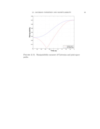
![2.5. JACOBIAN CONDITION AND MANIPULABILITY 24
−4
−2
0
2
4
−4
−2
0
2
4
−1
−0.5
0
0.5
1
Theta 1 (rad)Theta 2 (rad)
sqrt(det(J11))
Figure 2.7. 3D profile of the manipulability index measure of RRT
configuration.
a wider range of tasks within the workspace by avoiding the singular configurations.
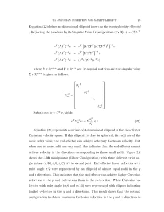
2.5. Jacobian Condition and Manipulability
The Jacobian linear system v “ Jpqq 9q maps the joint velocities to end-effector
Cartesian velocity. The Jacobian is regarded as scaling the input q to yield the
output. In a multidimensional case, the equivalent concept is to characterize the
output in terms of an input that has unit norm as follows [80]:
9q “ 9q2
1 ` 9q2
2 ` . . . ` 9q2
n ď 1 (21)
If the input (joint velocity) vector has unit norm, then the output (end-effector
velocity) will be positioned within an ellipsoid and defined :
9q 2
“ 9qT
9q
“ pJ`
vqT
J`
v
“ vT
pJJT
q´1
v (22)
where J`
is the Jacobian pseudo inverse and the derivation of Equation (22)
in Appendix (A). In particular, if the manipulator Jacobian is full rank, then](https://image.slidesharecdn.com/06f80bb7-ba1f-45e9-aa53-783373e47302-151229194001/85/Final-44-320.jpg)
![CHAPTER 3
Reconfigurable Robot Dynamics
In this chapter, the dynamics of a reconfigurable open kinematic robot is devel-
oped and analyzed following the method given by Djuric, Al Saidi and ElMaraghy
[38]. The motor that actuates the jth
hybrid joint exerts a torque that causes the
outward link, j, to accelerate and also exerts a reaction on the inwards link j ´ 1.
Gravity acting on the outward links j to n exert a weight force, and rotating links
also exert gyroscopic forces on each other. The resulting inertia from the motor
exertion is a function of the configuration of the outward links.
3.1. Reconfigurable Global Dynamic Model
The Global Dynamic Model (n-GDM) includes the link’s masses, m1, m2, . . . , mn
and center of masses, PC1, PC2, . . . , PCn. The center of mass PC1 is between joint
1 and joint 2, PC2 is between joint 2 and joint 3,..., etc., up to the last link. The
coordinates of any center of mass PCi is defined relative to the joint i ` 1 frame:
(xi`1, yi`1, zi`1). For the n-GDM model, which includes n reconfigurable joints,
the center of mass can be in 24 different places between any two successive joints.
This means that for each selection of the zi`1 coordinate frames, there are four
possible centers of mass: P1
Ci, P2
Ci, P3
Ci, P4
Ci. To find the center of mass of each
link for the n-GDM model, all possible coordinate frames are included and for all
joints. The analysis was done for the center of mass between joint 1 and joint 2.
The same procedure can be applied to the other n ´ 1 center of mass. A selection
of the z1
0 axis can support four different x-axis: x11
0 , x12
0 , x13
0 , x14
0 . For joint 2,
there are four different combinations of x1: x11
1 , x12
1 , x13
1 , x14
1 . Each of the four
x-combinations has four more combinations of the joint 2 coordinate frame. In
total there are sixteen different combinations of the first coordinate frame. By ob-
serving the coordinates of each center of mass, P1
C1, P2
C1, P3
C1, and P4
C1, relative to
31](https://image.slidesharecdn.com/06f80bb7-ba1f-45e9-aa53-783373e47302-151229194001/85/Final-51-320.jpg)
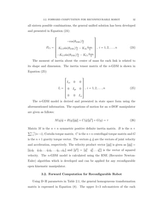
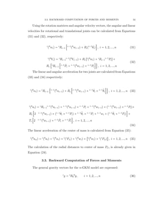
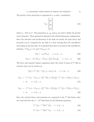
![3.3. BACKWARD COMPUTATION OF FORCES AND MOMENTS 36
Torques τi and forces fi are obtained by projecting the moments and forces onto
their corresponding joint axes respectively:
τi “ i
pi´1
niqT i´1
Zi´1, i “ 1, 2, ..., n (45)
fi “ i
pi´1
fiqT i´1
Zi´1, i “ 1, 2, ..., n (46)
The RNE procedure produced the final n expressions of the actuators’ torques and
forces τi, i “ 1, 2, . . . , n. Each of these n equations contains the sum of products
of the matrices’ elements M, B, C, G, and trigonometric terms. To be able to get
a dynamic equation in the form of Equation (26), each matrix was generated i.e.
M, B, C, and G, and their elements were calculated:
m11, m12, . . . , m1n, . . . , mnn, b112, b113, . . . , b1pn´1qn, . . . , bnpn´1qn,
c11, c12, . . . , c1n, . . . , cnn, g1, g2, . . . , gn.
To avoid complications when factoring out each element in each expression, the
Automatic Separation Method (ASM) is used, which produces an automatic gen-
eration of matrix elements [38]. Using the Newton-Euler recursive method for
calculating the forces and/or torques of the links for any open kinematic chain will
result n-equations. Each equation is a solution for force and/or torque of the link,
which includes four elements: the first one is related to inertia force/torque vector,
the second one is related to Coriolis force/torque vector, the third one is related
to centrifugal force/torque vector and the fourth one to gravity force/torque vec-
tor. These results will be coupled with the dynamics of different motors to form
a block diagram for control purposes. The elements of the matrices of the inertia
matrix, Coriolis matrix, centrifugal matrix and the gravity vector were calculated
to construct a complete block diagram of a robot. For these calculation, the ASM
method was used by starting the calculation of angular acceleration elements re-
lated the inertia, Coriolis centrifugal and gravity elements, Equations (53)-(60).
This procedure has three steps. The first step is to simplify and organize the an-
gular and linear velocity equations. To overcome these problems it is necessary to](https://image.slidesharecdn.com/06f80bb7-ba1f-45e9-aa53-783373e47302-151229194001/85/Final-56-320.jpg)
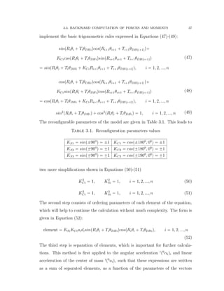
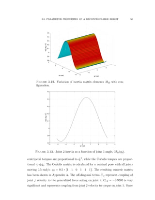
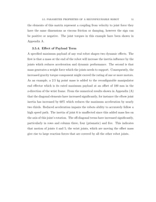
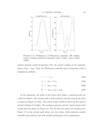
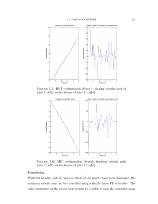
![3.5. PARAMETER PROPERTIES OF A RECONFIGURABLE ROBOT 45
of the third link, which as acts as a load, but otherwise independent of the third
joint.
3.5. Parameter Properties of a Reconfigurable Robot
The equations of motion (E.O.M) of various manipulators derived in the previ-
ous sections, can be described with a set of coupled differential equations in matrix
form:
τ “ Mpqq:q ` Cpq, 9qq ` F 9q ` Gpqq (71)
where q, 9q and :q are respectively the vector of generalized joint coordinates, ve-
locities and accelerations. M is the joint-space inertia matrix, C is the Coriolis
and centripetal coupling matrix, F is the friction force, G is the gravity loading,
and τ is the vector of generalized actuator torques associated with the generalized
coordinates q. This equation describes the manipulator rigid-body dynamics and
is known as the inverse dynamics, given the pose, velocity and acceleration it com-
putes the required joint forces and torques. In the previous sections, An efficient
reconfigurable recursive Newton-Euler algorithm was developed to compute the
Equation (71) for any open kinematic chain manipulator. This algorithm starts at
the base and working outwards adds the velocity and acceleration of each joint in
order to determine the velocity and acceleration of each link. Then working from
the tool back to the base, it computes the forces and moments acting on each link
and thus the joint torques.
In this section, the effect of varying configurations on dynamic parameters such
as the inertia and gravity load terms of a reconfigurable manipulator is analyzed
and investigated thoroughly. The D–H parameters of a predefined kinematic struc-
ture (PUMA 560) are given in Table 3.13 by Corke [33]. Using these parameters,
the workspace of the first three revolute joints and links is calculated and shown
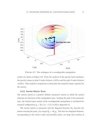
in Figure 3.6. The workspace of a reconfigurable robot manipulator with simi-
lar kinematic structure to the PUMA 560 is also calculated and shown in Figure
3.7. The resulting variable workspace shows a union of three layers that indicates
the workspace variability property of any reconfigurable manipulator. The three
workspace layers are calculated based on turning the third joint into a prismatic](https://image.slidesharecdn.com/06f80bb7-ba1f-45e9-aa53-783373e47302-151229194001/85/Final-65-320.jpg)
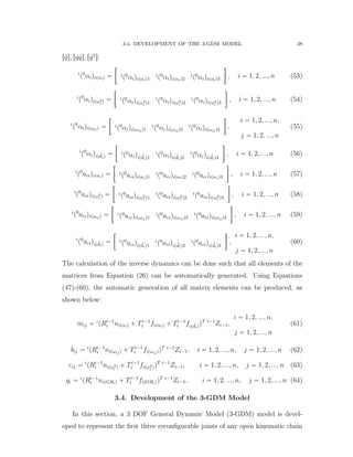
![3.5. PARAMETER PROPERTIES OF A RECONFIGURABLE ROBOT 46
Table 3.13. D–H parameters of the PUMA 560 Manipulator,
source; Fu, [41].
Joint j θj dj aj αj Joint range
1 θ1 0.3302 0 -π{2 -160 to +160
2 θ2 0 0.2032 0 -225 to 45
3 θ3 -0.05 0 π{2 -45 to 225
4 θ4 0.2032 0 -π{2 -110 to 170
5 θ5 0 0 π{2 -100 to 100
6 θ6 0 0 0 -226 to 266
Figure 3.6. The workspace of a predefined kinematic structure of
the PUMA 560.
one (translational motion). This variable workspace was generated when the third
joint has translated with 0.1, 0.2, 0.3 m.
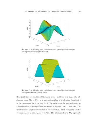
3.5.1. Gravity Load Term
Gravity load term in Equation (71) is generally a dominant term and present
even when the manipulator is stationary or moving slowly. The torque on a joint
due to gravity acting on the robot depends strongly on the robot’s pose. The
torque on the shoulder joint 2 is much greater when the robot is stretched out
horizontally as shown in Figure 3.8. The gravity torque on the elbow is high when
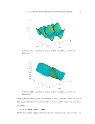
the pose changes due to joint reconfiguration from revolute to prismatic as the](https://image.slidesharecdn.com/06f80bb7-ba1f-45e9-aa53-783373e47302-151229194001/85/Final-66-320.jpg)
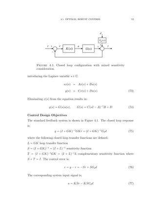
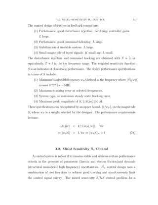
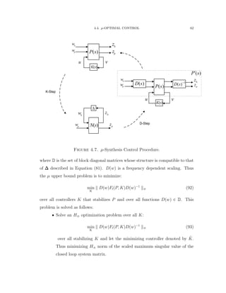
![4.2. MIXED SENSITIVITY H8 CONTROL 55
reconfigurable robot is to find a stabilizing controller K that minimizes [75]:
min
Kstabilizing
›
›
›
›
›
›
›
pI ` GKq´1
KpI ` GKq´1
›
›
›
›
›
›
›
8
(79)
where the sensitivity function S “ pI ` GKq´1
is shaped along with the closed
loop function transfer function KS. This cost function can be interpreted as the
design objectives of nominal performance (without Uncertainties), good tracking
or disturbance rejection, and robust stabilizing with additive uncertainties. The
sensitivity function S is the transfer function between the disturbance d and the
output y as shown in Figure 4.1. The KS is the transfer function between d and
control signal u. The KS function is regarded as a mechanism for limiting the
gain and bandwidth of the controller, and hence the control energy used. A scalar
high pass (weighting) filter is designed with a crossover frequency approximately
equal to that of the desired closed loop system. The disturbance d is usually a low
frequency signal, and therefore it will be rejected if the maximum singular value of
S is made small over the same low frequencies. A scalar low pass filter (weighting)
function wp is selected with a bandwidth equal to that of the disturbance frequency.
yu
w z
( )K s
( )P s
Figure 4.2. General H8 control configuration.
By combining these two objectives in one cost function Equation (79), the
problem is to find a stabilizing control that minimizes this cost function while
achieving the required performance. In order to implement a unified solution
procedure, the above cost function is recast into a standard H8 configuration
shown in Figure 4.2. The solution can be obtained by using the LFT (Linear
Fractional Transform) technique, in which the signals are classified into sets of
external inputs, outputs, input to the controller and output from the controller.](https://image.slidesharecdn.com/06f80bb7-ba1f-45e9-aa53-783373e47302-151229194001/85/Final-75-320.jpg)
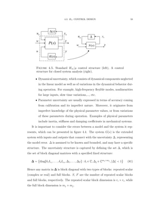
![4.3. H8 CONTROL DESIGN 56
The external inputs (reference and disturbance) are denoted by w, the output
signals to be minimized which includes both performance and robustness measures,
y is the vector of measurements available to the controller K and u the vector of
control signals. Ppsq is called the generalized plant or interconnected system. The
objective is to find a stabilizing controller K to minimize the output z over all w
with energy less than or equal to 1. This is equivalent to minimizing the H8-norm
of the transfer function from w to z. The mixed sensitivity problem [75] shown in
Figure 4.3 (left) is formulated to reject the disturbance when w “ d. The output
error signal is defined as z “
»
—
–
z1
z2
fi
ffi
fl, where z1 “ wpy and z2 “ ´wuu. It is also
calculated that z1 “ wpSw and z2 “ wuKSw and the elements of the generalized
plant P are:
»
—
—
—
—
—
–
z1
z2
v
fi
ffi
ffi
ffi
ffi
ffi
fl
“
»
—
—
—
—
—
–
wp wpG
0 ´wu
´I ´G
fi
ffi
ffi
ffi
ffi
ffi
fl
»
—
–
w
u
fi
ffi
fl
Then:
z “ FlpP, Kqw “ rP11 ` P12KpI ´ P22Kq´1
P21sw
where the FlpP, Kq is the lower linear fractional transformation of P and K:
FlpP, Kq “
»
—
–
wpS
wuKS
fi
ffi
fl (80)
Another formulation of the S{KS mixed sensitivity optimization is in the stan-
dard tracking control form as shown in Figure 4.3 (right). This is a tracking prob-
lem in which the input signal is the reference command r and the error signals are
z1 “ ´wpe “ wppr ´ yq and z2 “ wuu. The results of the tracking problem is to
minimize z1 “ wpSr and z2 “ wuKSr.
4.3. H8 Control Design
This section is mainly concerned with the design of an H8 feedback control to
stabilize the closed loop of a linear reconfigurable robot in the presence of uncertain](https://image.slidesharecdn.com/06f80bb7-ba1f-45e9-aa53-783373e47302-151229194001/85/Final-76-320.jpg)
![4.3. H8 CONTROL DESIGN 57
u
w r 1z
G
K
2z
e r y
P
pw
uw
w d
u
1z
G
K
2z
0r
e r y
P
uw
pw
y
v e v e
Figure 4.3. S/SK mixed sensitivity optimization in regulation
form (left), S/SK mixed sensitivity minimization in tracking form
(right).
u y( )G s
( )s
yu
Figure 4.4. Uncertain system representation.
parameters. The robust stability of the resulting closed loop has been analyzed
based on the structured singular value µ approach [75]. The nominal and robust
performance were also analyzed based on the minimizing of performance criteria
functions such the sensitivity and limiting control functions.
Uncertain Systems
For control design purposes, the possibly complex behavior of dynamical systems
must be approximated by models of relatively low complexity. The difference be-
tween such models and the actual physical system is called the model uncertainty.
Another cause of uncertainty is the imperfect knowledge of some components of
the system, or the change of their behavior due to changes in operating condi-
tions. Uncertainty also originates from physical parameters whose value is only
approximately known or varies in time. There are two major classes of uncertainty:](https://image.slidesharecdn.com/06f80bb7-ba1f-45e9-aa53-783373e47302-151229194001/85/Final-77-320.jpg)
![4.3. H8 CONTROL DESIGN 60
H8-Norm
A measure for the gain of a stable system N is the H8 norm, defined as:
}N}8 “ sup
}u}2ą0
}Nu}2
}u}2
(85)
which can be viewed as the largest possible amplification that N will induce, given
the worst-case input signal uptq. It is shown by Qu [69], that:
}N}8 “ sup
wPR
¯σpNpjwqq (86)
where ¯σ denotes the largest singular value. If N22 represents a nominal closed loop
system, then }N22}8 ď 1 indicates that the performance requirements have been
met (Nominal Performance).
µ-Norm
An important question is whether a nominal stable transfer function N, as defined
in Equation (82) remains stable for all ∆ P ∆ and if not, what the smallest size is
of a perturbation that can destabilize N. This is defined by the structured singular
value µ:
µ∆pN11q´1
“ min
∆
t¯σp∆q|detpI ´ N11∆q “ 0 for structured ∆ : ¯σp∆q ď 1u (87)
An uncertain closed loop system has been shown in Figure 4.6 where the input
w is to describe the disturbance and reference signals, z is the output to describe
the error signal. Robust stability, nominal performance and robust performance
are analyzed as follows:
‚ Robust stability (RS) is achieved if µ∆pN11pjwqq ď 1, @w.
‚ Nominal performance (NP) is achieved if }N22pjwq} ď 1, @w.
‚ Robust performance (RP) is achieved if µ∆e pNpjwqq ď 1, @w
where ∆e “
$
’&
’%
¨
˚
˝
∆ 0
0 ∆p
˛
‹
‚ ∆ P ∆∆∆, }∆p} ă 1,
,
/.
/-
.
where the performance complex uncertainty ∆p has the performance channel di-
mension of pdim r ` dim dq ˆ pdim e ` dim uq.](https://image.slidesharecdn.com/06f80bb7-ba1f-45e9-aa53-783373e47302-151229194001/85/Final-80-320.jpg)
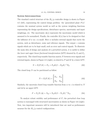
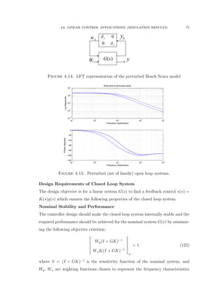
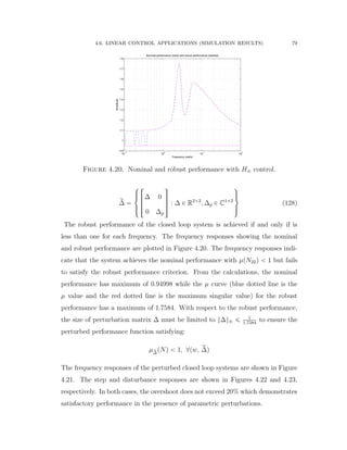
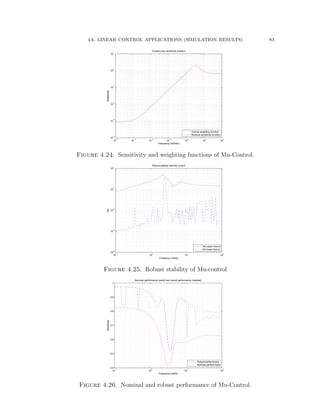
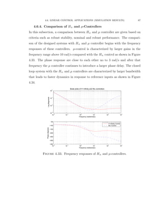
![4.6. LINEAR CONTROL APPLICATIONS (SIMULATION RESULTS) 70
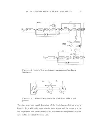
4.6. Linear Control Applications (Simulation Results)
4.6.1. Application of Mixed Sensitivity H8 Control (Simulation and
Results)
The Bosch Scara robot with RRT kinematic structure is considered based on the
experimental setup published in [73]. The first two joints and links are shown in
Figure 4.9 and the third joint is considered to be mechanically decoupled from the
motions of the other joints. The inertia and Coriolis matrices are given as follows:
Mpθq “
»
—
–
I1 ` 2I2 cospθ2q I3 ` I2 cospθ2q
I3 ` I2 cospθ2q I3
fi
ffi
fl (117)
Cpθ, 9θq “
»
—
–
´2I2 sinpθ2q 9θ1
9θ2 ´ I2 sinpθ2q 9θ2
1
I2 sinpθ2q 9θ2
1
fi
ffi
fl (118)
The complete system of the first two links is shown in Figure 4.9, including
servo motors with gearboxes, and the dynamic cross-coupling torques (Coriolis
effects). A spring-damper is introduced to model the torsion stiffness of the robot
shaft between each DC motor and the link. The dynamic coupling appears in the
joint systems as torques on the joint axes and is considered as an independent
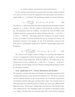
disturbance torque. The nominal values of the robot parameters are estimated at
the null position of the first two joints shown in Figure 4.10 and given in Table
A.1. The state equations of the first link is derived as follows:
9x1 “ x2
9x2 “
1
JL1
pKsx3 ` DsN1x4 ´ Fv1x2 ` τDLq
9x3 “ N1x4 ´ x2
9x4 “
1
Jm1
pKm1x5 ´ N1k5x3 ´ Fv1x4q
9x5 “
1
Lm1
p´Rm1x5 ´ Km1x4 ` x6 ` Kp12u ´ Kp12x5q
9x6 “ ´ki12x5 ` ki12u
y “ x1 (119)](https://image.slidesharecdn.com/06f80bb7-ba1f-45e9-aa53-783373e47302-151229194001/85/Final-90-320.jpg)

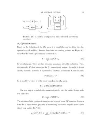
![4.6. LINEAR CONTROL APPLICATIONS (SIMULATION RESULTS) 94
1
3
K
K
( ( ))P t
pW
,q q
dq
dq
e
u
e
LPV SystemLPV Control
uˆu
uW
fW
Input Filter LPV Feedback
Linearized Syetem
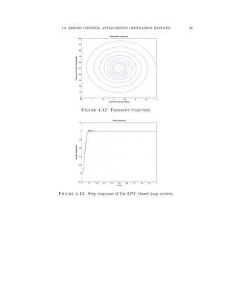
Figure 4.41. LPV control structure includes the LPV system
Ppθptqq, performance weighting functions Wp, robustness function
Wu, and LPV polytopic controllers (K1pθptqq, ¨ ¨ ¨ , K3pθptqq and in-
put filter Wf .
(2) To enforce the performance and robustness requirements by minimizing
the L2-gain of the closed loop performance channel.
These objectives should be satisfied for the time varying trajectories Mpqq and
Fp 9qq. The design procedure is performed with describing the LPV system Ppθptqq
Equation (119) by two affine parameter-dependent models. Using the LPV loop
shaping procedure, the resulting LPV polytopic system is placed within a polytope
convex hull of four vertex systems CotPi, i “ 1, ¨ ¨ ¨ , 4u. The vertices Pi are the
values of Ppθptqq at the four vertices (the four corners P1, ¨ ¨ ¨ , P4q of the following
parameter box:
p1 “
»
—
–
Mmax
Fmax
fi
ffi
fl , p2 “
»
—
–
Mmin
Fmax
fi
ffi
fl
p3 “
»
—
–
Mmax
Fmin
fi
ffi
fl , p4 “
»
—
–
Mmin
Fmin
fi
ffi
fl (134)
The LPV synthesis problem illustrated in Figure 4.41 is solved using the Mat-
lab/LMI control toolbox. To solve this problem, the input should be parameter
independent [43]. This condition is satisfied by prefiltering the control input u](https://image.slidesharecdn.com/06f80bb7-ba1f-45e9-aa53-783373e47302-151229194001/85/Final-114-320.jpg)
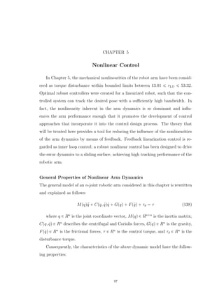
![5.1. POSITION CONTROL 98
‚ Highly nonlinear: each element of (138) contains nonlinear factors such
as trigonometric functions, and other mathematical models such as satu-
ration, square functions,..., etc.
‚ High degree of coupling between the dynamics of adjacent joints and links.
‚ Model uncertainty and time-variance: the load will vary when the robot
moves the objects or when the joint friction torque changes over time.
The mathematical formation of these characteristics are:
‚ The inertia matrix Mpqq is a positive definite, symmetric and bounded
matrix, i.e. there exists positive constants m1 and m2 such that m1I ď
Mpqq ď m2I.
‚ The centrifugal and Coriolis matrix Cpq, 9qq is bounded, i.e., there exits a
known cbpqq such that |Cpq, 9qq 9q| ď cbpqq} 9q}.
‚ The matrix 9M ´ 2C is a skew-symmetric matrix, i.e., xT
p 9M ´ 2Cqx “ 0,
where x is a vector.
‚ The known disturbance is satisfied with }τd} ď τM , where τM is a known
positive constant.
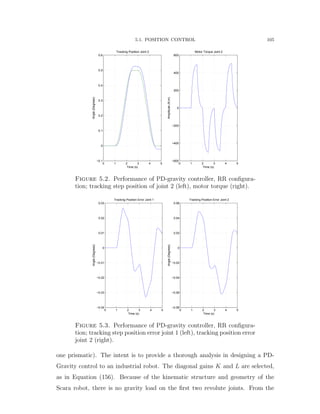
5.1. Position Control
The position control problem is considered by designing a PD-Gravity control
based on a Lyapunov function [74]. The resulting control compensates the gravity
element and assures step tracking, and linear and curvature trajectories satisfying
the required performance specifications. In Section 5.1.1, the dynamics of a servo
DC motor is combined with the link dynamics to form a compact servo mechanism
description. The derivation of the position control is given in Section 6.20 and the
simulation results have been presented in Subsections 5.1.3 and 5.1.4.
5.1.1. Link Dynamics. Let qi denote the generalized coordinate variable of
the hybrid joint and τi is the actuator torques vector of the n-axes of an open
kinematic structure robot. The general equation of motion can be rewritten as:
nÿ
j“1
Mijpqq :qj `
˜
nÿ
k“1
ÿ
j‰k
ckjpqq 9qk 9qj `
nÿ
k“1
ckkpqq 9q2
k
¸
` gipqq ` bip 9qq “ τi i “ 1...n
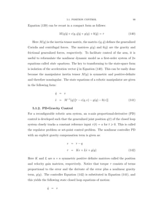
(139)](https://image.slidesharecdn.com/06f80bb7-ba1f-45e9-aa53-783373e47302-151229194001/85/Final-118-320.jpg)
![5.1. POSITION CONTROL 100
9v “ M´1
pqq rKpr ´ qq ` Lp9r ´ vq ´ cpq, vq ´ bpvqs (143)
Assume rptq “ a for t ě 0, for some set point a. To analyze the resulting equilib-
rium points of the closed loop system, the right hand side of the Equation (143)
is set to zero and solved for q and v. This yields:
v “ 0
M´1
pqq rKpa ´ qq ´ cpq, 0q ´ bp0qs “ 0 (144)
The Coriolis cpq, 0q “ 0 and bp0q “ 0, as they are functions of velocity with a
zero value at v “ 0. Thus, Kpa ´ qq “ 0 and the closed loop system has a single
equilibrium point:
pxT
“ raT
, 0T
s (145)
Then, the resulting equilibrium point at pxT
“
“
aT
, 0T
‰
of the closed loop system
represents the desired steady state solution of the nonlinear system when the
reference input is rptq. To satisfy the required performance of the closed loop
using the PD controller (142), it is sufficient to prove that the equilibrium point
pxT
is asymptotically stable and its domain of attraction encompasses the entire
state space [46].
Theorem: Let pxT
“
“
qT
, vT
‰
be the solution of the robotic arm described in
(141), assuming that τ is computed using the control law in (142). If rptq “ a for
t ě 0, then the equilibrium point pxT
“
“
aT
, 0T
‰
is asymptotically stable and the
domain of attraction is Ω “ R2n
. This means, for each xp0q P R2n
:
xptq Ñ px as t Ñ 8
Proof: the equilibrium point is first moved to the origin by letting, z “ q ´ a.
Then, the closed loop equations in (143) can be written in terms of z and v as:
9q “ 9v
9v “ ´M´1
pz ` aq rKz ` Lv ` cpz ` a, vq ` bpvqs (146)
Since cpz ` a, 0q “ 0 and bp0q “ 0, it follows that pz, vq “ p0, 0q is an equilibrium
point of the transform system (146). The Lyapunov function candidate (energy](https://image.slidesharecdn.com/06f80bb7-ba1f-45e9-aa53-783373e47302-151229194001/85/Final-120-320.jpg)
![5.1. POSITION CONTROL 101
function) is:
V pz, vq “
1
2
zT
Kz `
1
2
vT
Mpz ` aqv (147)
Since the inertia tensor Mpqq is a continuously differentiable positive definite ma-
trix and the position gain matrix K is also a positive definite matrix, it follows that
Equation (147) is a valid Lyapunov function, [51]. It is shown that the evaluation
of the function 9V pzptq, vptqq decreases along the solutions of the state Equation
(146) as follows:
9V pz, vq “
d
dt
ˆ
zT
Kz ` vT
Mpz ` aqv
2
˙
9V pz, vq “ zT
K 9z ` vT
Mpz ` aq9v `
vT 9Mpz ` aqv
2
9V pz, vq “ zT
Kv ´ vT
rKz ` Lv ` cpz ` a, vq ` bpvqs `
vT 9Mpz ` aqv
2
9V pz, vq “ pzT
KvqT
´ vT
rKz ` Lv ` cpz ` a, vq ` bpvqs `
vT 9Mpz ` aqv
2
9V pz, vq “ vT
KT
z ´ vT
rKz ` Lv ` cpz ` a, vq ` bpvqs `
vT 9Mpz ` aqv
2
9V pz, vq “ vT
Kz ´ vT
rKz ` Lv ` cpz ` a, vq ` bpvqs `
vT 9Mpz ` aqv
2
9V pz, vq “
vT 9Mpz ` aqv
2
´ vT
rLv ` cpz ` a, vq ` bpvqs
9V pz, vq “ vT
«
9Mpz ` aqv
2
´ cpz ` a, vq
ff
´ vT
rLv ` bpvqs (148)
The Coriolis and centrifugal torque term cpz ` a, vq can be expressed in terms
of 9Mpqq and a skew-symmetric matrix Npq, vq, yielding:
cpz ` a, vq “
1
2
r 9Mpz ` a, vq ´ Npz ` a, vqsv (149)
Substituting Equation (149) in Equation (148) yields:
9V pz, vq “
1
2
vT
Npz ` a, vqv ´ vT
rLv ` bpvqs (150)
The first term does not contribute to 9V pz ` a, vq because it is a skew matrix:
NT
pq, vq “ ´Npq, vq, which is given as follows:
vT
Npz ` a, vqv “
1
2
vT
Npz ` a, vqv `
1
2
vT
Npz ` a, vqv](https://image.slidesharecdn.com/06f80bb7-ba1f-45e9-aa53-783373e47302-151229194001/85/Final-121-320.jpg)
![5.1. POSITION CONTROL 102
vT
Npz ` a, vqv “
1
2
vT
Npz ` a, vqv `
1
2
rvT
Npz ` a, vqvsT
vT
Npz ` a, vqv “
1
2
vT
Npz ` a, vqv `
1
2
vT
NT
pz ` a, vqv
vT
Npz ` a, vqv “
1
2
vT
Npz ` a, vqv ´
1
2
vT
Npz ` a, vqv
vT
Npz ` a, vqv “ 0 (151)
Combining equations (150) and (151), the expression for 9V pz, vq along the
solution of the closed loop state equation in (143) reduces into:
9V pz, vq “ ´vT
rLv ` bpvqs (152)
9V pz, vq “ ´rvT
Lv ` vT
bpvqs (153)
Since L is positive definite and the friction coefficient is nonnegative, then
9V pz, vq ď 0 along the solution of closed loop system (143). From Equation (153),
the following yields:
9V pz, vq ” 0 ñ vptq ” 0
ñ 9vptq ” 0
ñ M´1
pzptq ` a, 0qKzptq ” 0
ñ zptq ” 0 (154)
Consequently, the equilibrium point pz, vq “ p0, 0q is asymptotically stable.
The domain of attraction is the set Ω where:
Ω “ tpz, vq : V pz, vq ă ρu
Ω “
"
pz, vq :
zT
Kz ` vT
Mpz ` aqv
2
ă ρ
*
(155)
Here, V pz, vq is a Lyapunov function and the asymptotic stability conditions
[51] are satisfied on Ωp for every ρ ą 0. Since K and Mpz ` a, vq are positive
definite matrices, V pz, vq Ñ 8 as }z} ` }v} Ñ 8. Thus, the domain of attraction
is the entire state space Ω “ R2n
. This implies, the equilibrium point pq, vq “ pa, 0q
is asymptotically stable.](https://image.slidesharecdn.com/06f80bb7-ba1f-45e9-aa53-783373e47302-151229194001/85/Final-122-320.jpg)
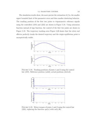
![5.2. TRAJECTORY CONTROL 108
0 1 2 3 4 5
−0.05
0
0.05
0.1
0.15
0.2
0.25
0.3
Error of Tracking Circular Path Joint 1
Time (s)
Angle(Degrees)
0 1 2 3 4 5
−5
−4
−3
−2
−1
0
1
x 10
−3 Error Joint 2
Time (s)
Angle(Degrees)
Figure 5.7. RRT configuration (Scara); tracking circular path
error joint 1 (left), tracking circular path error joint 2 (right).
K and L be symmetric positive definite matrices. The practical significance of the
PD-gravity control Equation (142) lies that it requires no detailed knowledge of
the manipulator inertia tensor Mpqq, the Coriolis and centrifugal coupling vector
cpq, vq, or the friction vector bvpq but it does require knowledge of the gravity
loading vector hpqq.
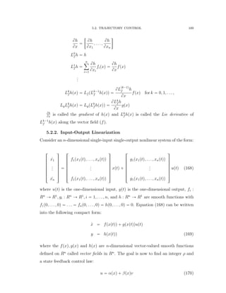
5.2. Trajectory Control
5.2.1. Feedback Linearization Control
One of the results of differential geometric nonlinear control theory [49, 62] con-
cerns the equivalence of nonlinear systems with linear systems, in case of feedback.
The (input-output) feedback linearization utilizes the feedback transforms (invert-
ibility of the system) to render linear input-output dynamics.
Mathematical Preliminaries Some mathematical preliminaries will be in-
troduced related to the differential geometry [4]: Suppose that h : Rn
Ñ R1
is a
smooth scalar function and f : Rn
Ñ Rn
, g : Rn
Ñ Rn
are vector fields, then:](https://image.slidesharecdn.com/06f80bb7-ba1f-45e9-aa53-783373e47302-151229194001/85/Final-128-320.jpg)
![5.2. TRAJECTORY CONTROL 112
5.2.3. Sliding Mode Control (SMC)
One approach to robust control design is called sliding mode control (SMC) method-
ology, which is also a type of variable structure control system (VSCS) [76]. The
most significant feature of SMC is the complete insensitivity to parametric uncer-
tainty and external disturbances during the sliding mode. The VSCS uses a high
speed switching control law to achieve two objectives. Firstly, it drives the nonlin-
ear system’s state trajectory along a specified and user chosen surface in the state
space which is called the sliding or switching surface. This surface is named the
switching surface because a control path has one gain if the state trajectory of the
system is above the surface and a different gain if the trajectory drops below the
surface. Secondly, it maintains the system’s state trajectory on this surface for all
subsequent times. During the process, the control system’s structure varies from
one to another and therefore it grants the name variable structure control. The
feedback linearization control law (178) achieves asymptotic tracking by satisfying
the error equation (175). Next, a sliding surface in Rn
is defined as follows:
sptq “ epρ´1q
ptq ` αpρ´1qepρ´2q
` ¨ ¨ ¨ ` α1eptq ` α0
ż
eptqdt “ 0 (179)
where αρ´1, . . . , α0 are such that:
λρ
` αpρ´1qλpρ´1q
` ¨ ¨ ¨ ` α1λ ` α0
is a Hurwitz polynomial. The derivative of the sliding surface sptq is given by:
9sptq “ epρq
ptq ` αpρ´1qepρ´1q
ptq ` ¨ ¨ ¨ ` α1ep1q
ptq ` α0eptq (180)
To satisfy the asymptotic tracking objective, the requirement is:
9sptq “ 0 (181)
Now, instead of satisfying the tracking error equation (175), a sliding condition is
described as follows:
Sliding Condition. There exists a positive number µ such that
1
2
ds2
dt
ď ´µ|s| (182)](https://image.slidesharecdn.com/06f80bb7-ba1f-45e9-aa53-783373e47302-151229194001/85/Final-132-320.jpg)
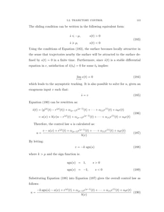
![5.2. TRAJECTORY CONTROL 114
From Equation (190), the tracking control law (178) can be viewed as a special case
of the sliding mode control by letting k “ 0 in Equation (190). The discontinuity
of the sign function will cause chattering in the closed loop system. In practice,
the sign function is often replaced by a saturation function sat(s{ ), where sat(.)
is defined as follows:
satpxq “ x, if |x| ď 1
satpxq “ sgnpxq, if |x| ą 1 (191)
Using this replacement will introduce tracking error. Trade-offs between the track-
ing error and control bandwidth can be made by suitably selecting the boundary
layer.
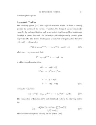
5.2.3.1. Linearity in Parameters
The dynamic parameters of a reconfigurable robot are not constant and function
of the robot configuration. The robot dynamics (71) can be written in the form
[80]:
Mpqq:q ` Cpq, 9qq 9q ` Gpqq “ Y pq, 9q, :qqϕ (192)
where Y pq, 9q, :qq is an nˆr matrix of known time functions and ϕ is an rˆ1 vector
of unknown constant parameters. This property is formulated by Graig [46] in
that it shows the separation of unknown parameters and known time functions.
The reason that the robot dynamics can be separated in this form is that the
robot dynamics are linear in the parameters expressed in the vector form ϕ. This
separation of unknown parameters and known time functions will be used in the
formulation of the adaptive update rule.
5.2.4. Sliding Mode Control Based on Estimated Model
In this subsection, sliding mode controllers are derived based on estimated models
and a 3-DOF reconfigurable robot is simulated to track a trigonometric reference
signal. For the desired trajectory as qdptq, the tracking error is defined as follows:
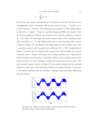
e “ qd ´ q](https://image.slidesharecdn.com/06f80bb7-ba1f-45e9-aa53-783373e47302-151229194001/85/Final-134-320.jpg)
![5.2. TRAJECTORY CONTROL 115
Define the reference velocity [76]:
9qr “ 9qd ` Λpqd ´ qq (193)
Where Λ is a positive diagonal matrix. Define a parameter vector error to be
˜ϕ “ pϕ ´ ϕ, where pϕ is the estimated vector of ϕ. According to the parametric
linear property, the robotic dynamic equation is now formulated as:
Mpqq:qr ` Cpq, 9qq 9qr ` Gpqq “ Y pq, 9q, :qqϕ (194)
And the dynamic error equation is:
˜Mpqq:qr ` ˜Cpq, 9qq 9qr ` ˜Gpqq “ Y pq, 9q, :qq ˜ϕ (195)
Where ˜Mpqq “ Mpqq ´ xMpqq, ˜Cpqq “ Cpqq ´ pCpqq and ˜Gpqq “ Gpqq ´ pGpqq.
Define the sliding surface s as:
s “ 9e ` Λe (196)
Select the Lyapunov function as:
V ptq “
1
2
sT
Mpqqs (197)
The Lyapunov function derivative is:
9V ptq “
1
2
”
sT
Mpqq9s ` sT 9Mpqq ` 9sT
Mpqqs
ı
(198)
Using the symmetric property of matrices:
9V ptq “
1
2
”
2sT
Mpqq9s ` sT 9Mpqqs
ı
(199)
9V ptq “ sT
Mpqq9s `
1
2
sT 9Mpqqs (200)
Since s “ 9q ´ 9qr and 9s “ :q ´ :qr, then:
9V ptq “ sT
pMpqq:q ´ Mpqq:qrq `
1
2
sT 9Mpqqs (201)](https://image.slidesharecdn.com/06f80bb7-ba1f-45e9-aa53-783373e47302-151229194001/85/Final-135-320.jpg)
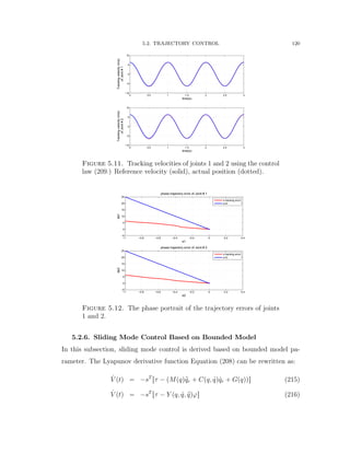
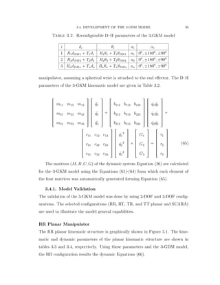
![5.2. TRAJECTORY CONTROL 126
−2 0 2 4 6 8 10 12 14
x 10
−3
−0.4
−0.2
0
0.2
0.4
0.6
0.8
1
e1
de1
s tracking error
s=0
−2 0 2 4 6 8 10 12 14
x 10
−3
−0.4
−0.2
0
0.2
0.4
0.6
0.8
1
e2
de2
s tracking error
s=0
Figure 5.20. Trajectory errors of joints 1 and 2.
5.2.8. Adaptive Control.
Adaptive control is an approach to control systems, which have constant or slowly-
varying uncertain parameters [76]. The basic theory in adaptive control is to esti-
mate the uncertain system parameters on-line based on measured system signals,
and exploit the estimated parameters in the control input computation. Thus, an
adaptive control can be regarded as a control with on-line parameters estimations
which maintain consistent performance of a system in the presence of uncertainty
or unknown variation in system parameters. The resulting dynamic parameters
of a reconfigurable manipulator are uncertain and time varying due to the con-
figuration change and joint pose dependency. This leads to consider the adaptive
control approach as a way of automatically adjusting the controller parameters in
the face of changing robot dynamic parameters. An adaptive control system is de-
picted schematically in Figure 5.21. It is composed of three parts: a reconfigurable
robot with unknown parameters, a feedback control law containing adjustable pa-
rameters, and an adaptation mechanism for updating the adjustable parameters.
The operation of the adaptive controller is as follows: at each time instant, the
estimator sends to the controller a set of estimated system parameters pϕ, which
was calculated based on the system input τ and output q, 9q. The controller finds
its corresponding parameters and then computes a control input τ based on the
controller parameters and measured signals. The control input τ causes a new](https://image.slidesharecdn.com/06f80bb7-ba1f-45e9-aa53-783373e47302-151229194001/85/Final-146-320.jpg)
![5.2. TRAJECTORY CONTROL 127
Reconfigurable
Robot
ˆ
ˆ ˆˆ
r rMq Cq G
DKs e e
ˆ T
Y s
, ,d d dq q q
,q q
Adaptation Law
Controller
ˆ
Figure 5.21. Control structure diagram of the adaptive control.
system output to be generated and whole cycle of parameter estimation and input
updates is repeated.
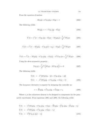
5.2.9. Derivation of Adaptive Sliding Mode Control
An adaptive controller is derived and developed for a 3-DOF reconfigurable ro-
bot described in tables 3.2 and 3.1. The trajectory control problem is solved by
developing a robust controller for the actuator joints, and an estimation law for
the unknown parameters, such that the manipulator output qptq closely tracks the
desired trajectory qdptq. The tracking error is defined as in Equation (196). Define
the reference velocity [76]:
9qr “ 9qd ` Λpqd ´ qq (226)
Where Λ is a positive diagonal matrix:
Λ “ diag pλ1, λ2, ¨ ¨ ¨ , λnq, λi ą 0
The sliding variable is defined as:
s “ 9e ` Λe](https://image.slidesharecdn.com/06f80bb7-ba1f-45e9-aa53-783373e47302-151229194001/85/Final-147-320.jpg)
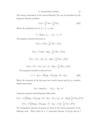
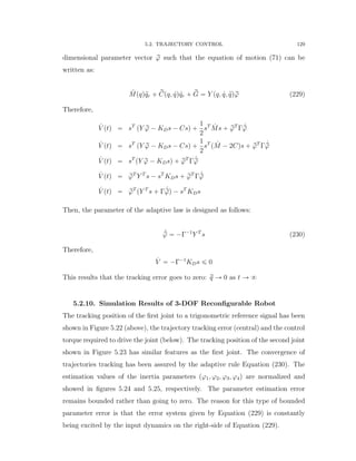
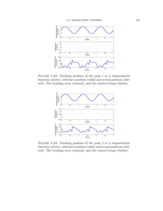
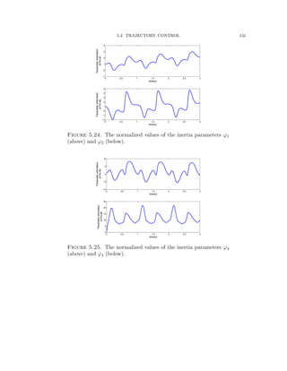
![CHAPTER 6
Kinematic and Control Selection Algorithm
To realize a reconfigurable robot, an algorithm has been developed that com-
bines the selection of an applicable kinematic structural robot configuration with
control design methods to optimize robot capability and performance. Assuming
a spherical wrist attached to the end effector, the kinematic structures of common
industrial robots are determined by the first three links and joints, which also
define the external and internal workspace boundaries. A spherical wrist; which
satisfies Piper’s condition [45] when a4 “ 0, a5 “ 0 and d5 “ 0; only serves to
orient the end effector within the workspace. The resulting reconfigurable robot
includes eight kinematic structures: Cartesian TTT, Cylindrical RTT, TTR, TRT,
Articulated RRR, Spherical/Scara RRT, TRR, and RTR.
In this chapter, an algorithm with configuration and control phases is developed
to select an optimal kinematic configuration structure with the most applicable
control approach to perform a specified trajectory with high tracking performance.
6.1. Configuration Phase
The configuration algorithm shown in Figure 6.1 starts by defining the geo-
metric task in terms of its shape, dimensions, etc. To build the entire trajectory
sequentially, the task is divided into segments according to trajectory shape (lin-
ear/curvature). To perform the first segment, the algorithm begins with the TTT
kinematic structure. The kinematic model for this structure can be automatically
generated using the generic kinematic algorithm developed in Chapter 2. The
workspace of the kinematic structure is calculated from the Cartesian coordinates
of the position vector partitioned from the homogeneous matrix transformation.
Then, the workspace singularity of the configuration is evaluated by calculating the
determinant of the Jacobian. The reachability property of the segment within the
workspace is tested by calculating the inverse kinematics of the structure. In case
132](https://image.slidesharecdn.com/06f80bb7-ba1f-45e9-aa53-783373e47302-151229194001/85/Final-152-320.jpg)
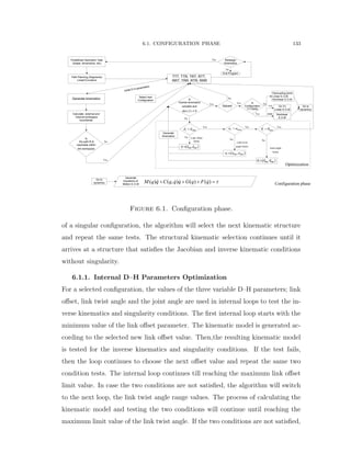
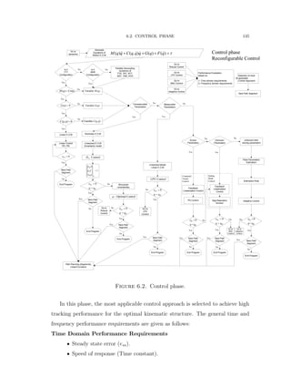
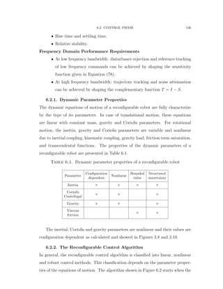
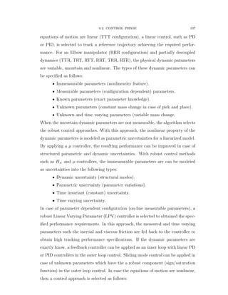
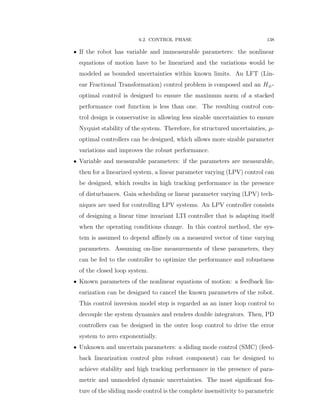
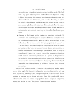
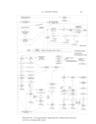
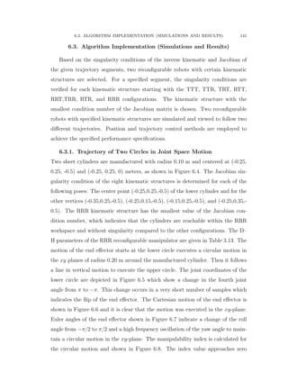
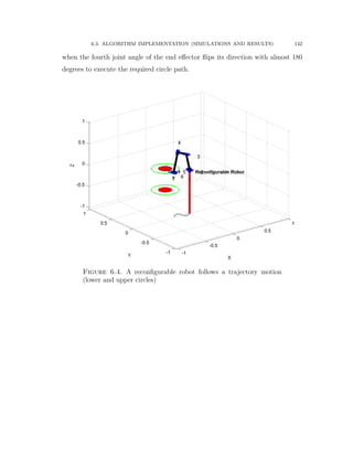
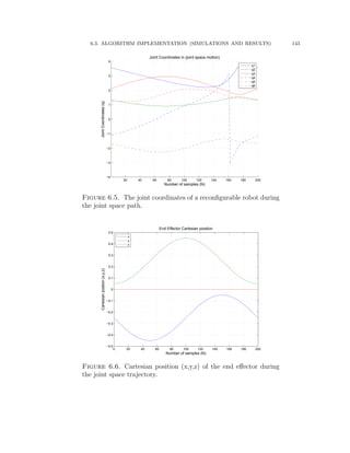
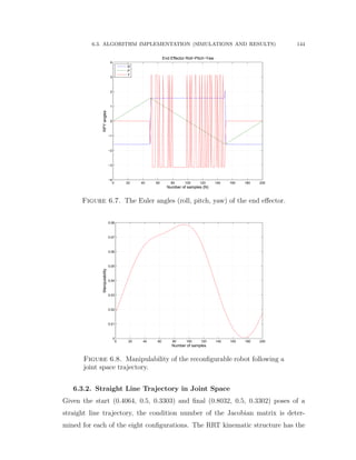
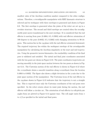
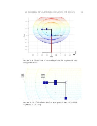
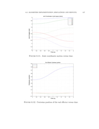
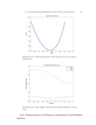
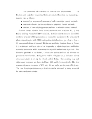
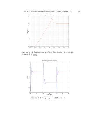
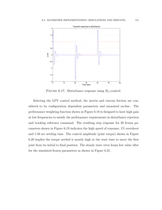
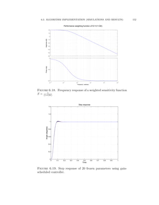
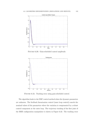
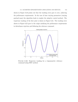
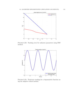
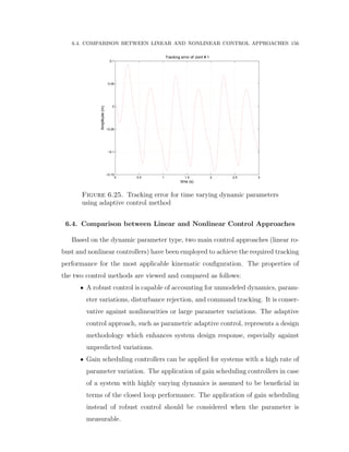
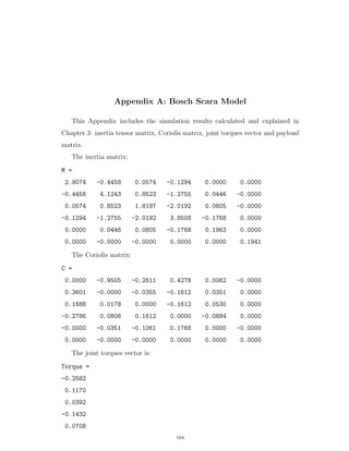
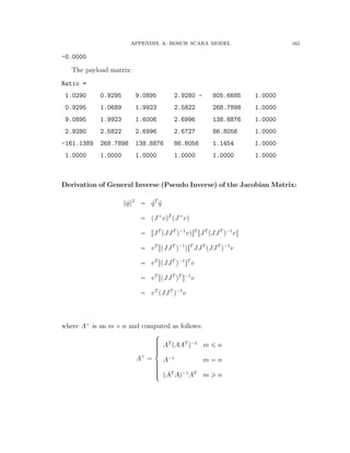
![Appendix B: Bosch Scara Model
In this Appendix, the parameters of the Bosch Scara robot are given with
the state space representation of the linearized model. Table A.1 includes the
parameter values of the first two links and joints. The parameters of the first two
DC motors are given in Table A.2.
Table A.1. Nominal parameter values of the Bosch Scara robot arm
Servo/ Link 1 Value Units
Fv1 0.001 Nms/rad
FvL
90 Nms/rad
Km1 0.24 Nm/A
Rm1 1.45 Ω
Jm1 1.075 10´2
kgm2
Lm1 ď 1.5 10´3
H
N1 129´1
[1]
L1 0.445 m
Servo/ Link 2 Value Units
Fv2 0.005 Nms/rad
Km2 0.099 Nm/A
Rm2 1.87 Ω
Jm2 4.2 10´4
kgm2
Lm2 ď 1.0 10´4
H
N2 101´1
[1]
L2 0.355 m
Table A.2. Nominal parameter values of the Bosch Scara robot arm
Amplifier 1 Value Units
KP11 27.9 [1]
KI11 646.5 sec´1
τ1 8 10´5
sec´1
KP12 1.42 V/A
KI12 227 V/As
Amplifier 1 Value Units
KP21 28 [1]
KI21 413.3 sec´1
τ2 8 10´5
sec´1
KP22 2.67 V/A
KI22 280 V/As
166](https://image.slidesharecdn.com/06f80bb7-ba1f-45e9-aa53-783373e47302-151229194001/85/Final-186-320.jpg)
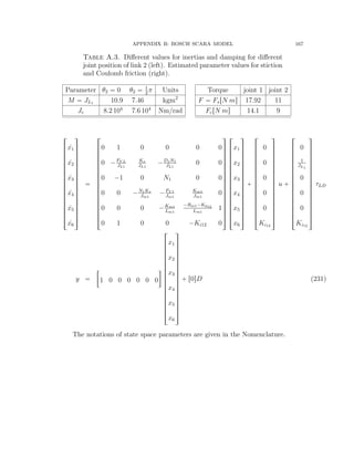
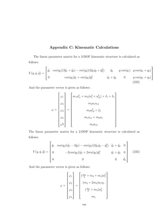
![References
[1] C. Abdallah, D. Dawson, P. Dorato, and M. Jamshidi, Survey of robust control for rigid
robots, IEEE Control Systems Magazine, 11 (1991), 24-29.
[2] C. Abdallah, D. Dawson, P. Dorato, and M. Jamshidi, Survey of robust control of robots,
Proceedings of American Control Conference, (1990), 718-721.
[3] K. Abdel-Malik, H. J. Yeh, Analytical Boundary of the Workspace for General 3-DOF Mech-
anism, The International Journal of Robotics Research, 16 (1997), 198-213.
[4] R. Abraham and J.E. Marsden, Foundation of Mechanics (2nd edition), The Benjamin
Cummings Publishing Company, 1978.
[5] F. Aghili and K. Parsa, A Reconfigurable Robot with Lockable Cylindrical Joints, IEEE
Transactions on Robotics 25 (2009), 785-797.
[6] P. Apkarian, P. Gahinet, A convex characterization of gain-scheduled H8 controllers, IEEE
Trans. Automat. Control. (1995), 853-864.
[7] R. Al Saidi and B. Minaker, Analysis of Generic kinematic for self-reconfigurable open
kinematic machinery systems, Proc. 24th
Canadian Congress of Applied Mechanics, (2013).
[8] R. Al Saidi and B. Minaker, Analysis and development of self-reconfigurable open kinematic
machinery systems, Proc. IEEE International Conference on Automation Science and En-
gineering, (2013), 966-971.
[9] R. Al Saidi and B. Minaker, Development and control of self-reconfigurable open kinematic
chain robot arms, Proc. IEEE International Symposium on Robotic and Sensors Environ-
ments, (2013).
[10] R. Al Saidi and B. Minaker, An adaptive sliding mode control for trajectory tracking of a
self-reconfigurable robotic system, Robot Intelligence Technology and Applications 2: Results
from the 2nd
International Conference on Robotic Intelligence Technology and Applications,
Ed. J–H Kim, E. T. Matson, H. Myung, P. Xu and F. Karray, Springer, (2013), 381-391.
[11] R. Al Saidi and B. Minaker, Kinematic properties and control for a reconfigurable robotic
system, Proc. IEEE International Conference on Systems, Man and Cybernetics, (2014),
2827-2832.
[12] R. Al Saidi and B. Minaker, Analysis and control of a reconfigurable robotic arm, J. Au-
tonomous Robots, (2014), Submitted.
[13] R. O. Ambrose, Interactive Robot Joint Design, Analysis and Prototyping, IEEE Interna-
tional Conference on Robotics and Automation, (1995), 2119-2124.
169](https://image.slidesharecdn.com/06f80bb7-ba1f-45e9-aa53-783373e47302-151229194001/85/Final-189-320.jpg)
![REFERENCES 170
[14] R. J. Anderson and J.B. Moore, Passive computed torque algorithms for robots, Proceedings
of the IEEE Conference on Decision and Control, (1989), 1638-1644.
[15] J. Angeles, Fundamentals of Robotic Mechanical Systems: Theory, Methods, and Algorithms,
3rd ed. New York: Springer-Verlag, 2007.
[16] J. Angeles, A methodology for the optimum dimensioning of robotic manipulators, Univ.
Autonoma de San Luis Potos, San Luis Potos, Mexico, Memoria del 5o. Congreso Mexicano
de Robotica, (2003), 190203.
[17] S. Arimoto. Control theory of non-linear mechanical systems: a passivity-based circuit the-
oretic approach, Clarendon-Press, Oxford, 1996.
[18] B. Benhabib, G. Zak, and M. G. Lipton, A Generalized Kinematic Modeling Method for
Modular Robots, J. Robotics Systems 6 (1989), 545-571.
[19] H. Berghuis, Model based robot control: from theory to practice, PhD thesis, University of
Twente, The Netherlands, 1993.
[20] Z. M. Bi, W. A. Gruver and S. Y. T. Lang, Analysis and Synthesis of Reconfigurable Robotic
Systems, Robotics and Computer-Integrated Manufacturing 12 (2010), 553-562.
[21] Z. M. Bi, W. A. Gruver, W.J. Zhang, A.Y.T. Lang, Automated modeling of modular robotic
configurations, Robotics and Autonomous Systems 54 (2006), 1015-1025.
[22] Z. M. Bi, W. J. Zhang, I-M. Chen and S. Y. T. Lang, Automated Generation of the D–H
Parameters for Configuration Design of Modular Manipulators, Robotics and Computer-
Integrated Manufacturing 23 (2007), 553-562.
[23] S.P. Boyd and C.H. Barrat, Linear controller design; limits of performance, Prentice-Hall,
1991.
[24] C. Canudas de Wit, B. Siciliano, and G. Bastin. Theory of Robot Control, Springer, 1996.
[25] M. Ceccarelli, A Formulation for the Workspace Boundary of General n-Revolute Manipu-
lators, Mechanism and Machine Theory 31 (1996), 637-646.
[26] M. Ceccarelli and A., Vinciguerra, On the Workspace of 4R manipulators, The International
Journal of Robotics Research 14 (1995) 152-160.
[27] I-M. Chen, Theory and Applications of Modular Reconfigurable Robotic Systems, PhD thesis,
California Institute of Technology, USA, 1994.
[28] I-M. Chen and J. W. Brudick, Rapid response manufacturing through a rapidly reconfigurable
robotic work cell, Robotics and Computer-Integrated Manufacturing 3 (2001), 199-213.
[29] I-M. Chen and J. W. Burdick, Enumerating the Non-Isomorphic Assembly Configurations of
Modular Robotic Systems, Proceedings of IEEE/RSJ International Conference on Intelligent
Robots and Systems (IROS), (1993), 1985-1992.
[30] B. S. Chen, T. S. Lee, and J. H. Feng, A nonlinear H8 control design in robotic systems
under parameter perturbation and external disturbance, International Journal of Control 59
(1994), 439-461.](https://image.slidesharecdn.com/06f80bb7-ba1f-45e9-aa53-783373e47302-151229194001/85/Final-190-320.jpg)
![REFERENCES 171
[31] I-M. Chen and G. Yang, Configuration Independent Kinematics for Modular Robots, IEEE
International Conference on Robotics and Automation, (1996) 1440-1445.
[32] R. Cohen, M. G. Lipton, M. Q. Dai and B. Benhabib, Conceptual Design of a Modular
Robot, ASME Journal of Mechanical Design 114, (1992), 117-125.
[33] P. Corke and B. Armstrong-Helouvry, A search for consensus among model parameters
reported for PUMA 560, Proc. IEEE Int. Conf. Robotics and Automation, (1994), 1608-
1613.
[34] Corke. P, Robotic toolbox, (2002).
[35] J. Denavit, R.S. Hartenberg, A kinematic notation for lower-pair mechanisms based on
matrices, Journal of Applied Mechanics, (1955) 215-221.
[36] A. Djuric, Reconfigurable kinematics, dynamics and control process for industrial robots,
PhD dissertation, University of Windsor, (2007)
[37] A. Djuric, R. Al Saidi and W. ElMaraghy, Global Kinematic Model Generation of n-DOF
Reconfigurable Machinery Structure, Proc. IEEE International Conference on Automation
Science and Engineering, (2010), 804-809.
[38] A. Djuric, R. Al Saidi and W. ElMaraghy, Dynamics solution of n-DOF global machinery
model, Robotics and Computer-Integrated Manufacturing 28, (2012), 621-630.
[39] H. A. ElMaraghy, Changeable and Reconfigurable Manufacturing systems, Springer Verlag.,
New York, 2009.
[40] B. Friedland, Control System Design, MacGraw Hill, 1986.
[41] K. S. FU, R. C. Gonzalez, C. S. G. Lee, Robotics Control, Sensing, Vision, and Intelligence,
MacGraw Hill, 1987.
[42] T. Fukuda and S. Nakagawa, Dynamically Reconfigurable Robotic System, IEEE Interna-
tional Conference on Robotics and Automation, (1988), 1581-1586.
[43] P. Gahinet, P. Apkarian, Self-scheduled H8 control of linear parameter varying systems,
Proc. Amer. Control. Conference. (1994), 856-860.
[44] M. T. Grabbe and D. M. Dawson, An application op optimal control theory to the trajectory
of rigid robot manipulator, Optimal Control Application & Methods 15 (1994), 237-249.
[45] J. Graig, Introduction to Robotics, Mechanics and Control, Addison-Wesley, 1989.
[46] J. Graig, Adaptive Control of Mechanical Manipulators, Englewood Cliffs, NJ: Prentice Hall,
1989.
[47] K. C. Gupta and B. Roth, Design consideration for manipulator workspace, ASME J. Mech.
Design, 104, (1982), 704712.
[48] M. Hedelind and M. Jackson, The need for Reconfigurable Robotic Systems, Proc. Of the
2nd Int. Conf. on Changeable, Agile, Reconfigurable and Virtual Production, CARV (2007).
[49] A. Isidori, Nonlinear Control Systems: An Introduction, Lecture notes in Control and In-
formation Science, 72, (1985) Springer Verlag.](https://image.slidesharecdn.com/06f80bb7-ba1f-45e9-aa53-783373e47302-151229194001/85/Final-191-320.jpg)
![REFERENCES 172
[50] Z. Jing and J. Yi, Dimensional synthesis based on fault tolerant performance for redundant
robots, Procedings 13th Int. Conf. Adv. Robot., (2007), 10231028.
[51] H. K. Khalil, Nonlinear systems, 3rd Edition, Prentice Hall, N.J., 2002.
[52] Koren Y., Heisel U., Jovane F., Moriwaki T., Pritschow G., Ulsoy G., van Brussel H.,
Reconfigurable Manufacturing Systems. Annals of the CIRP, 48/2, (1999), 527540.
[53] K. Kreutz. On manipulator control by exact linearization, IEEE Transactions on Automatic
Control 34 (1989), 763767.
[54] M. Krstic, I. Kanellakopoulos, and P. Kokotovic. Nonlinear and Adaptive Control Design,
Wiley, 1995.
[55] A. Kumar and K. J. Waldron, The workspace of a mechanical manipulator, ASME J. Mech.
Design 103, (1981), 665672.
[56] S. J. Kwon, W. K. Chung, Y. Youm, and M. S. Kim, Self-collision avoidance for n-link
redundant manipulators, Proceedings of the IEEE Systems, Man, Cybern., Decision Aiding
Complex System., Charlottesville, VA, Oct. (1991), 937942.
[57] F. Lewis, C. Abdallah, and D. Dawson. Control of Robot Manipulators, Macmillan, 1993.
[58] Z. Li, W. Melek, and C. M. Clark, Development and Characterization of a Modular and
Reconfigurable Robot, Proceedings of the International Conference on Changeable, Agile,
Reconfigurable and Virtual Production, CARV (2007).
[59] G. Liu, Development of modular and reconfigurable with multiple working modes Proceedings
of IEEE Int. Conf. Robotics and Automation, (2008).
[60] J. M. Maciejowski, Multivariable Feedback Design, Addison-Wesley, 1989.
[61] J.-P. Merlet, Parallel Robots, 2nd ed. New York: Springer-Verlag, 2006.
[62] H. Nijmeijer and A. J. van der Schaft, Nonlinear Dynamical Control Systems, (1990)
Springer Verlag.
[63] R. Manseur, Robot Modeling and Kinematics, De Vinci Engineering Press, 2006.
[64] R. Manseur and K. L. Doty, Structural Kinematics of 6-Revolute-Axis Robot Manipulators.
Mechanism and Machine Theory 31 (1996), 647-657.
[65] R. M. Murray, Z. Li, and S. S. Sastry. A Mathematical Introduction to Robotic Manipulation,
CRC, 1994.
[66] R. Ortega and R. Spong, Adaptive motion control of rigid robots, Proceedings of the IEEE
Conference on Decision and Control, (1988), 1575-1584.
[67] C. J. J. Paredis, H. B. Brown, R. W. Casciola, J. E. Moody and P. K. Khosla, A Rapidly De-
ployable Manipulator System, International Workshop on Some Critical Issues in Robotics,
(1995), 175-185.
[68] Z. Qu, Global stability of trajectory tracking of robot under PD control, Proceedings of IEEE
Conference of Control Applications, (1992), 8-12.](https://image.slidesharecdn.com/06f80bb7-ba1f-45e9-aa53-783373e47302-151229194001/85/Final-192-320.jpg)
![REFERENCES 173
[69] Z. Qu, Global stabilization of nonlinear systems with a class of unmatched uncertainties,
Proceedings of IEEE Conference of Control Applications, (1992), 498-503.
[70] Z. Qu and D. M. Dawson. Robust Tracking Control of Robot Manipulators. IEEE-Press,
1996.
[71] Z. Qu and J. Dorsey, Robust tracking control of robots by a linear feedback law, IEEE Trans-
actions on Automatic Control 36 (1992), 1081-1084.
[72] M. C. Readman, Flexible Joint Robots, CRC, 1994.
[73] Theodorus A, Robot Trajectory Planning, PhD thesis, Delft University of Technology, 1992.
[74] R. J. Schilling, Fundamentals of robotics, Prentice Hall, 1990
[75] S. Skogestad, I. Postlethwait, Multivariable Feedback Control, Analysis and Control, John
Wiley & Sons, 1997.
[76] J. E. Slotine and W. Li, Applied Nonlinear Control, Prentice Hall, N.J., 1991
[77] J. J. E. Slotine and J. J. Craig, Adaptive trajectory control of manipulators, The Robotics
Review 1 (1989), 369-377.
[78] Y. D. Song, A. T. Alouani and J. N. Anderson, Robust path tracking control of industrial
robots: an H8 approach, Proceedings of the IEEE Conference on Control Applications,
(1992), 25-30.
[79] M. W. Spong, Modeling and control of elastic joint robots, ASME Journal on Dyn., Sys.,
Measurement and Control 109 (1987), 310319.
[80] M. W. Spong, S. Hutchinson, M. Vidyasagar, Robot Modeling and Control, John Wiley &
Sons, 2006.
[81] M. Spong and M. Vidyasagar. Robot Dynamics and Control, Wiley, 1989.
[82] M. Spong and M. Vidyasagar, Robust linear compensator design for nonlinear robotic control,
IEEE Transactions on Robotics and Automation, (1985), 954-959.
[83] W. L. Stout and M. E.Swan, Application of H8 theory to robot manipulator control, Pro-
ceedings of the IEEE Conference on Control Applications, (1992) 148-153.
[84] T. Strasser, M. N. Rooker and G. Ebenhofer,Distributed Control Concept for a 6-DOF
Reconfigurable Robot Arm, Innovation production machines and systems: Fourth I*Proms
Virtual International Conference, (2008).
[85] S. Tabandeh, C. Clarck, and W. Melek, Task-based Configuration Optimization of Modular
and Reconfigurable Robots using a Multi-Solution Inverse Kinematics Solver, International
Conference on Changeable, Agile, Reconfigurable and Virtual Production. CARV (2007).
[86] V. I. Utkin, Sliding modes and their application in variable structure systems (English trans-
lation), MIR publications, 1978.
[87] K. H. Wurst, The Conception and Construction of a Modular Robot System, 16th Int. Sym.
Industrial Robotics (ISIR), (1986) 37-44.
[88] K. Zhou, J. Doyle, and K. Glover, Robust and Optimal Control, Prentice-Hall, 1996.](https://image.slidesharecdn.com/06f80bb7-ba1f-45e9-aa53-783373e47302-151229194001/85/Final-193-320.jpg)
![REFERENCES 174
[89] T. Yoshikawa, Manipulability of robotic mechanisms, The Journal of Robotics Research, 4,
(1985), 39.](https://image.slidesharecdn.com/06f80bb7-ba1f-45e9-aa53-783373e47302-151229194001/85/Final-194-320.jpg)


