Downloaded 11 times
![International Journal of Engineering Inventions
e-ISSN: 2278-7461, p-ISSN: 2319-6491
Volume 2, Issue 7 (May2013) PP: 68-73
www.ijeijournal.com Page | 68
Tuning of PID, SVFB and LQ Controllers Using Genetic
Algorithms
P. Kumar1
, O. N. Mehrotra2
, J. Mahto3
Abstract: The Inverted Pendulum is a very popular plant for testing dynamics and control of highly non-linear
plants. In the Inverted Pendulum Control problem, the aim is to move the cart to the desired position and to
balance a pendulum at desired location. This paper represents stabilization of pendulum using PID, SVFB and
LQR. An advantage of Quadratic Control method over the pole-placement techniques is that the former
provides a systematic way of computing the state feedback control gain matrix.LQR In the mathematical model
proposed here, a PID, SVFB and LQR controller is designed and all the controllers are tuned using Genetic
algorithms. The simulation results of all the controllers are shown. This paper exhibits the capability of genetic
algorithm to solve complex and constrained optimization problems and as a general purpose optimization tool
to solve control system design problems.
Keyword: Inverted pendulum (IP), Mathematical modeling, PID controller, State variable feedback controller
(SVFB), LQR, Genetic algorithm (GA).
I. INTRODUCTION
The inverted pendulum is unstable [8,9,10] in the sense that it may fall any time in any direction unless a
suitable control force is applied. If the designer works it right, he can get the advantages of several effects[11].
The control objective of the inverted pendulum is to swing up[4] the pendulum hinged on the moving cart by a
linear motor[11] from stable position (vertically down state) to the zero state (vertically upward state) and to
keep the pendulum in vertically upward state in spite of the disturbance[6,7]. They make it easy to check whether
a particular algorithm [5] yields the requisite results. Several works has been reported on the inverted pendulum
for its stabilization. Attempts have been made in the past to control it using classical control [3]. The purpose of
the present research is to tune[1,2] the entire controller by soft computing tools. The work was made under
MATLAB simulation.
II. MATHEMATICAL MODEL OF THE PLANT
Defining displacement of the cart as 𝑥, the angle of the rod from the vertical (reference) line as 𝜃 , the
force applied to the system as F , centre of gravity of the pendulum rod at its geometric centre and 𝑙 the half
length of the pendulum rod, the physical model of the system is shown in fig (1).
The Lagrangian of the entire system is given as,
L=
1
2
(𝑚𝑥2
+2𝑚𝑙𝑥 cos𝜃+𝑚𝑙2
𝜃2
+𝑀𝑥2
)+
1
2
𝐼𝜃2
]-𝑚𝑔𝑙cos𝜃
The Euler-Lagrange’s equation for the system is
𝑑
𝑑𝑡
𝛿𝐿
𝛿𝑥
−
𝛿𝐿
𝛿𝑥
+ 𝑏𝑥 = 𝐹 (1)
𝑑
𝑑𝑡
𝛿𝐿
𝛿𝜃
−
𝛿𝐿
𝛿𝜃
+ 𝑑𝜃 = 0 (2)
The dynamics of the entire system using above equation is
𝐼 + 𝑚𝑙2
𝜃 + 𝑚𝑙 cos 𝜃 𝑥 − 𝑚𝑔𝑙 sin 𝜃 + 𝑑𝜃 = 0 (3)
𝑀 + 𝑚 𝑥 + 𝑚𝑙 cos 𝜃 𝜃 − 𝑚𝑙 sin 𝜃 𝜃2
+ 𝑏𝑥 = 𝐹 (4)
In order to derive the linear differential equation model, the non linear differential equation obtained need to be
linearized. For small angle deviation around the upright equilibrium (fig.2) point, assumption made sin 𝜃 =
𝜃, cos 𝜃 = 1, 𝜃2
= 0
Using above relation, equation (5) and (6) are derived.
r𝜃+q𝑥-k𝜃+d =0 (5)
𝑝𝑥 + 𝑞𝜃 + 𝑏𝑥 = 𝐹 (6) Where, (𝑀
+ 𝑚)= p, 𝑚𝑔𝑙=k, 𝑚𝑙=q, 𝐼 + 𝑚𝑙2
= r
𝑥1 = 𝑥 + 𝑙 sin 𝜃](https://image.slidesharecdn.com/i02076873-130910042843-phpapp02/85/Tuning-of-PID-SVFB-and-LQ-Controllers-Using-Genetic-Algorithms-1-320.jpg)
![International Journal of Engineering Inventions
e-ISSN: 2278-7461, p-ISSN: 2319-6491
Volume 2, Issue 7 (May2013) PP: 68-73
www.ijeijournal.com Page | 68
Tuning of PID, SVFB and LQ Controllers Using Genetic
Algorithms
P. Kumar1
, O. N. Mehrotra2
, J. Mahto3
Abstract: The Inverted Pendulum is a very popular plant for testing dynamics and control of highly non-linear
plants. In the Inverted Pendulum Control problem, the aim is to move the cart to the desired position and to
balance a pendulum at desired location. This paper represents stabilization of pendulum using PID, SVFB and
LQR. An advantage of Quadratic Control method over the pole-placement techniques is that the former
provides a systematic way of computing the state feedback control gain matrix.LQR In the mathematical model
proposed here, a PID, SVFB and LQR controller is designed and all the controllers are tuned using Genetic
algorithms. The simulation results of all the controllers are shown. This paper exhibits the capability of genetic
algorithm to solve complex and constrained optimization problems and as a general purpose optimization tool
to solve control system design problems.
Keyword: Inverted pendulum (IP), Mathematical modeling, PID controller, State variable feedback controller
(SVFB), LQR, Genetic algorithm (GA).
I. INTRODUCTION
The inverted pendulum is unstable [8,9,10] in the sense that it may fall any time in any direction unless a
suitable control force is applied. If the designer works it right, he can get the advantages of several effects[11].
The control objective of the inverted pendulum is to swing up[4] the pendulum hinged on the moving cart by a
linear motor[11] from stable position (vertically down state) to the zero state (vertically upward state) and to
keep the pendulum in vertically upward state in spite of the disturbance[6,7]. They make it easy to check whether
a particular algorithm [5] yields the requisite results. Several works has been reported on the inverted pendulum
for its stabilization. Attempts have been made in the past to control it using classical control [3]. The purpose of
the present research is to tune[1,2] the entire controller by soft computing tools. The work was made under
MATLAB simulation.
II. MATHEMATICAL MODEL OF THE PLANT
Defining displacement of the cart as 𝑥, the angle of the rod from the vertical (reference) line as 𝜃 , the
force applied to the system as F , centre of gravity of the pendulum rod at its geometric centre and 𝑙 the half
length of the pendulum rod, the physical model of the system is shown in fig (1).
The Lagrangian of the entire system is given as,
L=
1
2
(𝑚𝑥2
+2𝑚𝑙𝑥 cos𝜃+𝑚𝑙2
𝜃2
+𝑀𝑥2
)+
1
2
𝐼𝜃2
]-𝑚𝑔𝑙cos𝜃
The Euler-Lagrange’s equation for the system is
𝑑
𝑑𝑡
𝛿𝐿
𝛿𝑥
−
𝛿𝐿
𝛿𝑥
+ 𝑏𝑥 = 𝐹 (1)
𝑑
𝑑𝑡
𝛿𝐿
𝛿𝜃
−
𝛿𝐿
𝛿𝜃
+ 𝑑𝜃 = 0 (2)
The dynamics of the entire system using above equation is
𝐼 + 𝑚𝑙2
𝜃 + 𝑚𝑙 cos 𝜃 𝑥 − 𝑚𝑔𝑙 sin 𝜃 + 𝑑𝜃 = 0 (3)
𝑀 + 𝑚 𝑥 + 𝑚𝑙 cos 𝜃 𝜃 − 𝑚𝑙 sin 𝜃 𝜃2
+ 𝑏𝑥 = 𝐹 (4)
In order to derive the linear differential equation model, the non linear differential equation obtained need to be
linearized. For small angle deviation around the upright equilibrium (fig.2) point, assumption made sin 𝜃 =
𝜃, cos 𝜃 = 1, 𝜃2
= 0
Using above relation, equation (5) and (6) are derived.
r𝜃+q𝑥-k𝜃+d =0 (5)
𝑝𝑥 + 𝑞𝜃 + 𝑏𝑥 = 𝐹 (6) Where, (𝑀
+ 𝑚)= p, 𝑚𝑔𝑙=k, 𝑚𝑙=q, 𝐼 + 𝑚𝑙2
= r
𝑥1 = 𝑥 + 𝑙 sin 𝜃](https://image.slidesharecdn.com/i02076873-130910042843-phpapp02/75/Tuning-of-PID-SVFB-and-LQ-Controllers-Using-Genetic-Algorithms-1-2048.jpg)

![Tuning of PID, SVFB and LQ Controllers Using Genetic Algorithms
www.ijeijournal.com Page | 73
References
[1] P.Kumar,O.N.Mehrotra,J.Mahto,’’Tuning of PID Controller Of Inverted Pendulum using Genetic algorithm”pp 359-363.IJRET,Voi
1,Issue 3,Dec 2012
[2] P.Kumar,O.N.Mehrotra,J.Mahto,’’ Controller design Of Inverted Pendulum using Pole placement and LQR”pp 532-538..IJRET,Voi
1,Issue 4,Dec 2012
[3] Kumar,P, Mehrotra , O.N, Mahto.J, Mukherjee, Rabi Ranjan,”Modelling and Controller Design of Inverted Pendulum”, National
Conference on Communication, Measurement and Control, Vol-I, 14th August, 2012
[4] S.Vivek Kumar Radha Mohan,Mona Subramaniam, “A clustering technique for digital communications channel equalization using
radial basis function networks,” IEEE Transactions Neural Networks, vol. 4, pp. 570-578, July 1993.
[5] Elmer P. Dadias, Patrick S. Fererandez, and David J,”Genetic Algorithm on Line Controller For The Flexible Inverted
Pendulum Problem”, Journal Of Advanced Computational Intelligence and Intelligent Informatics
[6] W. Wang, “Adaptive fuzzy sliding mode control for inverted pendulum,” in Proceedings of the Second Symposium International
Computer Science and Computational Technology(ISCSCT ’09) uangshan, P. R. China, 26-28, Dec. pp. 231-234, 2009
[7] Kumar.P, Mehrotra.O.N, Mahto.J, Mukherjee, Rabi Ranjan,”Stabilization of Inverted Pendulum using LQR”, National Conference
on Communication, Measurement and Control, Vol-I, 14th August, 2012.
[8] Stefani, Shahian, Savant, Hostetter :Design Of Feedback Control Systems,4th
edition, New York, Oxford University Press 2002
,Page (675 – 732)
[9] Behra Laxmidhar & Kar Indrani; Intelligent Systems and Control Principals and Applications; Oxford University Press
[10] Ogata, K.; System Dynamics, 4th
Edition Englewood Cliffs, NJ: Prentice-Hall, 2003
[11] Feedback instruments,U.K
Prof. Mehrotra, a Gold Medalist at B.Sc. Engineering(B.U), M.E.(Hons)(U.O.R) and Ph.D. (R.U) all in Electrical
Engineering, has the industrial exposure at SAIL as Testing & Commissioning Engineer. Served Department of Science
& Technology, Govt. of Bihar & Govt. of Jharkhand for 35 years and retired as Professor in Electrical Engineering.
Served as coordinator of various projects sanctioned through MHRD and AICTE, including TEQIP, a World Bank
Project. His research interests include control and utilization of renewable energies, power quality and power
system.Presently he is Director of Shivalik college of engineering Dehradun,Uttrakhand,India
Dr. Jagdeo Mahto was born in Madhubani, Bihar, India, in 1943. He obtained the B.Sc (Engg) degree in Electrical
Engineering from Bhagalpur University in 1964, M.Tech. in Control System from IIT Kharagpur, India in 1970 and
Ph.D in Control System in 1984 from IIT Delhi, India. He served MIT Muzaffarpur from 1964 to 1971 in the capacity of
Lecturer and Assistant Professor. From 1971 to 1980 he served as Asst. Professor, from 1980 to 1985 as Associate
Professor and from 1985 to 1988 as Professor in the Department of Electrical Engineering at BIT Sindri, India. He
taught at Bright Star University, Brega (Libya) from 1988 to 1989. From 1989 to 2003 he was again at BIT Sindri. From
2004 till date he is Professor at Asansol Engg. College
Pankaj Kumar was born in Muzaffarpur, India, in 1970 and received the B.Sc and M.Sc. degree in Electronics Honours
and Electronic Science respectively from Magadh University and Gauhati University Assam. He received M.Sc
Engineering in Control System Engineering from Patna University in 2004. He began his career as Lecturer in Bihar
University Muzaffarpur. Currently he is an Assistant Professor in the Department of Electrical Engineering, Asansol
Engineering College, Asansol, India.](https://image.slidesharecdn.com/i02076873-130910042843-phpapp02/85/Tuning-of-PID-SVFB-and-LQ-Controllers-Using-Genetic-Algorithms-6-320.jpg)
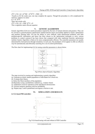
1) The document describes using genetic algorithms to tune PID, state variable feedback, and LQR controllers for balancing an inverted pendulum on a cart. 2) It presents the mathematical model of the inverted pendulum system and linearizes the model. 3) PID, state variable feedback, and LQR controllers are designed for the system. The controller parameters are then tuned using a genetic algorithm to minimize error. 4) Simulation results show the genetic algorithm approach improves rise time and reduces overshoot compared to controllers without genetic algorithm tuning.