SlideShare a Scribd company logo
ELECTRICAL
INSTRUMENTS
AND
MEASURE-
MENTS
Learning Objectives
➣
➣
➣
➣
➣ Absolute and Secondary
Instruments
➣
➣
➣
➣
➣ Deflecting Torque
➣
➣
➣
➣
➣ Controlling Torque
➣
➣
➣
➣
➣ Damping Torque
➣
➣
➣
➣
➣ Moving-iron Ammeters and
Voltmeters
➣
➣
➣
➣
➣ Moving-coil Instruments
➣
➣
➣
➣
➣ Permanent Magnet Type
Instruments
➣
➣
➣
➣
➣ Voltmeter Sensitivity
➣
➣
➣
➣
➣ Electrodynamic or
Dynamometer Type
Instruments
➣
➣
➣
➣
➣ Hot-wire Instruments
➣
➣
➣
➣
➣ Megger
➣
➣
➣
➣
➣ Induction Voltmeter
➣
➣
➣
➣
➣ Wattmeters
➣
➣
➣
➣
➣ Energy Meters
➣
➣
➣
➣
➣ Electrolytic Meter
➣
➣
➣
➣
➣ Ampere-hour Mercury Motor
Meter
➣
➣
➣
➣
➣ Friction Compensation
➣
➣
➣
➣
➣ Commutator Motor Meters
➣
➣
➣
➣
➣ Ballistic Galvanometer
➣
➣
➣
➣
➣ Vibration Galvanometer
➣
➣
➣
➣
➣ Vibrating-reed Frequency
Meter
➣
➣
➣
➣
➣ Electrodynamic Frequency
Meter
➣
➣
➣
➣
➣ Moving-iron Frequency Meter
➣
➣
➣
➣
➣ Electrodynamic Power Factor
Meter
➣
➣
➣
➣
➣ Moving-iron Power Factor
Meter
➣
➣
➣
➣
➣ Nalder-Lipman Moving-iron
Power Factor Meter
➣
➣
➣
➣
➣ D.C. Potentiometer
➣
➣
➣
➣
➣ A.C. Potentiometers
➣
➣
➣
➣
➣ Instrument Transformers
➣
➣
➣
➣
➣ Potential Transformers.
Electrical instruments help us to
measure the changes in variables
such as voltage, current and
resistance
©
10
C H A P T E R
376 ElectricalTechnology
10.1. Absolute and Secondary Instruments
The various electrical instruments may, in a very broad sense,
be divided into (i) absolute instruments and (ii) secondary
instruments. Absolute instruments are those which give the
value of the quantity to be measured, in terms of the constants
of the instrument and their deflection only. No previous
calibration or comparision is necessary in their case. The example
of such an instrument is tangent galvanometer, which gives the
value of current, in terms of the tangent of deflection produced
by the current, the radius and number of turns of wire used and
the horizontal component of earth’s field.
Secondary instruments are those, in which the value of
electrical quantity to be measured can be determined from the
deflection of the instruments, only when they have been pre-
calibrated by comparison with an absolute instrument. Without calibration, the deflection of such
instruments is meaningless.
It is the secondary instruments, which are most generally used in everyday work; the use of the
absolute instruments being merely confined within laboratories, as standardizing instruments.
10.2. Electrical Principles of Operation
All electrical measuring instruments depend for their action on one of the many physical effects
of an electric current or potential and are generally classified according to which of these effects is
utilized in their operation. The effects generally utilized are :
1. Magnetic effect - for ammeters and voltmeters usually.
2. Electrodynamic effect - for ammeters and voltmeters usually.
3. Electromagnetic effect - for ammeters, voltmeters, wattmeters and watthour meters.
4. Thermal effect - for ammeters and voltmeters.
5. Chemical effect - for d.c. ampere-hour meters.
6. Electrostatic effect - for voltmeters only.
Another way to classify secondary instruments is to divide them into (i) indicating instruments
(ii) recording instruments and (iii) integrating instruments.
Indicating instruments are those which indicate the instantaneous value of the electrical quantity
being measured at the time at which it is being measured. Their indications are given by pointers
moving over calibrated dials. Ordinary ammeters, voltmeters and wattmeters belong to this class.
Recording instruments are those, which, instead of indicating by means of a pointer and a scale
the instantaneous value of an electrical quantity, give a continuous record or the variations of such a
quantity over a selected period of time. The moving system of the instrument carries an inked pen
which rests lightly on a chart or graph, that is moved at a uniform and low speed, in a direction
perpendicular to that of the deflection of the pen. The path traced out by the pen presents a continu-
ous record of the variations in the deflection of the instrument.
Integrating instruments are those which measure and register by a set of dials and pointers either
the total quantity of electricity (in amp-hours) or the total amount of electrical energy (in watt-hours
or kWh) supplied to a circuit in a given time. This summation gives the product of time and the
electrical quantity but gives no direct indication as to the rate at which the quantity or energy is being
supplied because their registrations are independent of this rate provided the current flowing through
the instrument is sufficient to operate it.
Ampere-hour and watt-hour meters fall in this class.
An absolute instrument
Electrical Instruments and Measurements 377
10.3. Essentials of Indicating Instruments
As defined above, indicating instruments are those which indicate the value of the quantity that is
being measured at the time at which it is measured. Such instruments consist essentially of a pointer
which moves over a calibrated scale and which is attached to a moving system pivoted in jewelled
bearings. The moving system is subjected to the following three torques :
1. A deflecting (or operating) torque
2. A controlling (or restoring) torque
3. A damping torque.
10.4. Deflecting Torque
The deflecting or operating torque (Td) is produced by utilizing one or other effects mentioned in
Art. 10.2 i.e. magnetic, electrostatic, electrodynamic, thermal or inductive etc. The actual method of
torque production depends on the type of instrument and will be discussed in the succeeding para-
graphs. This deflecting torque causes the moving system (and hence the pointer attached to it) to
move from its ‘zero’ position i.e. its position when the instrument is disconnected from the supply.
10.5. Controlling Torque
The deflection of the moving system would be indefinite if there were no controlling or restoring
torque. This torque oppose the deflecting torque and increases with the deflection of the moving
system. The pointer is brought to rest at a position where the two opposing torques are equal. The
deflecting torque ensures that currents of different magnitudes shall produce deflections of the mov-
ing system in proportion to their size. Without such at torque, the pointer would swing over to the
maximum deflected position irrespective of the magnitude of the current to be measured. Moreover,
in the absence of a restoring torque, the pointer once deflected, would not return to its zero position
on removing the current. The controlling or restoring or balancing torque in indicating instruments is
obtained either by a spring or by gravity as described below :
(a) Spring Control
A hair-spring, usually of phosphor-
bronze, is attached to the moving
system of the instrument as shown in
Fig. 10.1 (a).
With the deflection of the pointer,
the spring is twisted in the opposite
direction. This twist in the spring
produces restoring torque which is
directly proportional to the angle of
deflection of the moving system. The
pointer comes to a position of rest (or
equilibrium) when the deflecting torque
(Td) and controlling torque (Tc) are equal.
For example, in permanent-magnet,
moving-coil type of instruments, the
deflecting torque is proportional to the
current passing through them.
∴ Td ∝I
and for spring control Tc ∝θ
As Tc = Td
∴ θ ∝ I
Fig. 10.1
378 ElectricalTechnology
Since deflection θ is directly proportional to current I, the spring-controlled instruments have a
uniform or equally-spaced scales over the whole of their range as shown in Fig. 10.1 (b).
To ensure that controlling torque is proportional to the angle of deflection, the spring should
have a fairly large number of turns so that angular deformation per unit length, on full-scale deflec-
tion, is small. Moreover, the stress in the spring should be restricted to such a value that it does not
produce a permanent set in it.
Springs are made of such materials which
(i) are non-magnetic
(ii) are not subject to much fatigue
(iii) have low specific resistance-especially in cases where they are used for leading current in or
out of the instrument
(iv) have low temperature-resistance coefficient.
The exact expression for controlling torque is Tc = Cθ where C is spring constant. Its value is
given by C =
3
Ebt
L
N-m/rad. The angle θ is in radians.
(b) Gravity Control
Gravity control is obtained by attaching a small adjustable weight to some part of the moving
system such that the two exert torques in the opposite directions. The usual arrangements is shown in
Fig. 10. 2(a).
It is seen from Fig. 10.2 (b) that the con-
trolling or restoring torque is proportional
to the sine of the angle of deflection i.e.
Tc ∝sin θ
The degree of control is adjusted by
screwing the weight up or down the carry-
ing system
It Td ∝ I
then for position of rest
Td = Tc
or I ∝ sin θ (not θ)
It will be seen from Fig. 10.2 (b) that as θ approaches 90º, the distance AB increases by a
relatively small amount for a given change in the angle than when
θ is just increasing from its zero value. Hence, gravity-controlled
instruments have scales which are not uniform but are cramped
or crowded at their lower ends as shown in Fig. 10.3.
As compared to spring control, the disadvantages of gravity
control are :
1. it gives cramped scale
2. the instrument has to be kept vertical.
However, gravity control has the following advantages :
1. it is cheap
2. it is unaffected by temperature
3. it is not subjected to fatigue or deterioration with time.
Example 10.1 The torque of an ammeter varies as the square of the current through it. If a
current of 5 A produces a deflection of 90º, what deflection will occur for a current of 3 A when the
instrument is (i) spring-controlled and (ii) gravity-controlled.
(Elect. Meas. Inst and Meas. Jadavpur Univ.)
Fig. 10.2
Fig. 10.3
Electrical Instruments and Measurements 379
Solution. Since deflecting torque varies as (current)
2
, we have Td ∝I
2
For spring control, Tc ∝ θ ∴ θ ∝ I
2
For gravity control, Tc ∝sin θ ∴ sin θ ∝ I2
(i) For spring control 90º ∝5
2
and θ ∝3
2
; θ = 90° × 3
2
/5
2
= 32.4º
(ii) For gravity control sin 90º ∝5
2
and sin θ ∝3
2
sin θ = 9/25 = 0.36 ; θ = sin−
1
(0.36) = 21.1º.
10.6. Damping Torque
A damping force is one which acts on the moving
system of the instrument only when it is moving and
always opposes its motion. Such stabilizing or demping
force is necessary to bring the pointer to rest quickly,
otherwise due to inertia of the moving system, the pointer
will oscillate about its final deflected position for quite
some time before coming to rest in the steady position.
The degree of damping should be adjusted to a value
which is sufficient to enable the pointer to rise quickly
to its deflected position without overshooting. In that
case, the instrument is said to be dead-beat. Any
increase of damping above this limit i.e. overdamping
will make the instruments slow and lethargic. In Fig. 10.4 is shown the effect of damping on the
variation of position with time of the moving system of an instrument.
The damping force can be produced by (i) air frictions (ii) eddy currents and (iii) fluid friction
(used occasionally).
Two methods of air-friction damping are shown in Fig. 10.5 (a) and 10.5 (b). In Fig.. 10.5 (a),
the light aluminium piston attached to the moving system of the instrument is arranged to travel with
Fig. 10.5
a very small clearance in a fixed air chamber closed at one end. The cross-section of the chamber is
either circular or rectangular. Damping of the oscillation is affected by the compression and suction
actions of the piston on the air enclosed in the chamber. Such a system of damping is not much
favoured these days, those shown in Fig. 10.5 (b) and (c) being preferred. In the latter method, one
or two light aluminium vanes are mounted on the spindle of the moving system which move in a
closed sector-shaped box as shown.
Fluid-friction is similar in action to the air friction. Due to greater viscosity of oil, the damping
is more effective. However, oil damping is not much used because of several disadvantages such as
objectionable creeping of oil, the necessity of using the instrument always in the vertical position and
its obvious unsuitability for use in portable instruments.
Fig. 10.4
Piston V
Air
Chamber
Control
Spring
Vanes
Sector Shaped
Box
Vane
(a) (b) (c)
380 ElectricalTechnology
The eddy-current form of damping is the most efficient of the three. The two forms of such a
damping are shown in Fig. 10.6 and 10.7. In Fig. 10.6 (a) is shown a thin disc of a conducting but
non-magnetic material like copper or aluminium mounted on the spindle which carries the moving
system and the pointer of the instrument. The disc is so positioned that its edges, when in rotation, cut
the magnetic flux between the poles of a permanent magnet. Hence, eddy currents are produced in
the disc which flow and so produce a damping force in such a direction as to oppose the very cause
producing them (Lenz’s Law Art. 7.5). Since the cause producing them is the rotation of the disc,
these eddy current retard the motion of the disc and the moving system as a whole.
Fig. 10.6
In Fig. 10.7 is shown the second type of
eddy-current damping generally employed
in permanent-magnet moving coil instru-
ments. The coil is wound on a thin light
aluminium former in which eddy currents
are produced when the coil moves in the
field of the permanent magnet. The direc-
tions of the induced currents and of the
damping force produced by them are shown
in the figure.
The various types of instruments and the
order in which they would be discussed in
this chapter are given below.
Ammeters and voltmeters
1. Moving-iron type (both for D.C./A.C.)
(a) the attraction type
(b) the repulsion type
2. Moving-coil type
(a) permanent-magnet type (for D.C. only)
(b) electrodynamic or dynamometer type (for D.C./A.C.)
3. Hot-wire type (both for D.C./A.C.)
4. Induction type (for A.C. only)
(a) Split-phase type
(b) Shaded-pole type
5. Electrostatic type-for voltmeters only (for D.C./A.C.)
Fig. 10.7
Electrical Instruments and Measurements 381
Wattmeter
6. Dynamometer type (both for D.C./A.C.),
7. Induction type (for A.C. only)
8. Electrostatic type (for D.C. only)
Energy Meters
9. Electrolytic type (for D.C. only)
10. Motor Meters
(i) Mercury Motor Meter. For d.c. work only. Can be used as amp-hour or watt-hour meter.
(ii) Commutator Motor Meter. Used on D.C./A.C. Can be used as Ah or Wh meter.
(iii) Induction type. For A.C. only.
11. Clock meters (as Wh-meters).
10.7. Moving-iron Ammeters and Voltmeters
There are two basic forms of these
instruments i.e. the attraction type and
the repulsion type. The operation of
the attraction type depends on the at-
traction of a single piece of soft iron
into a magnetic field and that of repul-
sion type depends on the repulsion of
two adjacent pieces of iron magnetised
by the same magnetic field. For both
types of these instruments, the neces-
sary magnetic field is produced by the
ampere-turns of a current-carrying coil.
In case the instrument is to be used as
an ammeter, the coil has comparatively fewer turns of thick wire so that the ammeter has low resis-
tance because it is connected in series with the circuit. In case it is to be used as a voltmeter, the coil
has high impedance so as to draw as small a
current as possible since it is connected in par-
allel with the circuit. As the current through
the coil is small, it has large number of turns
in order to produce sufficient ampere-turns.
10.8. Attraction Type M.I.
Insturments
The basic working principle of an attrac-
tion-type moving-iron instrument is illustrated
in Fig. 10.8. It is well-known that if a piece of
an unmagnetised soft iron is brought up near
either of the two ends of a current-carrying coil,
it would be attracted into the coil in the same
way as it would be attracted by the pole of a
bar magnet. Hence, if we pivot an oval-shaped
disc of soft iron on a spindle between bear-
ings near the coil (Fig. 10.8), the iron disc will
swing into the coil when the latter has an elec-
tric current passing through it. As the field
strength would be strongest at the centre of
Fig. 10.8
Moving iron ammeter
Moving iron voltmeter
382 ElectricalTechnology
the coil, the ovalshaped iron disc is pivoted in such a way that the greatest bulk of iron moves into the
centre of the coil. If a pointer is fixed to the spindle carrying the disc, then the passage of current
through the coil will cause the pointer to deflect. The amount of deflection produced would be
greater when the current producing the magnetic field is greater. Another point worth noting is that
whatever the direction of current through the coil, the iron disc would always be magnetised in
such a way that it is pulled inwards. Hence, such instruments can be used both for direct as well as
alternating currents.
A sectional view of the actual instrument is shown in Fig. 10.9. When the current to be measured
is passed through the coil or solenoid, a magnetic field is produced, which attracts the eccentrically-
mounted disc inwards, thereby deflecting the pointer, which moves over a calibrated scale.
Deflecting Torque
Let the axis of the iron disc, when in zero position, subtend an angle of φwith a direction perpen-
dicular to the direction of the field H produced by the coil. Let the deflection produced be θ corre-
sponding to a current I through the coil. The magnetisation of iron disc is proportional to the compo-
nent of H acting along the axis of the disc i.e. proportional to H cos [90 −(φ + θ)] or H sin (θ + φ).
The force F pulling the disc inwards is proportional to MH or H
2
sin (θ + φ). If the permeability of
iron is assumed constant, then, H ∝I. Hence, F ∝I
2
sin (θ + φ). If this force acted at a distance of l
from the pivot of the rotating disc, then deflecting torque Td = Fl cos (θ + φ). Putting the value of F,
we get
Td ∝I
2
sin (θ + φ) × l cos (θ + φ) ∝I
2
sin 2 (θ + φ) = KI
2
sin 2 (θ + φ) ...sin l is constant
If spring-control is used, then controlling torque Tc = K′ θ
In the steady position of deflection, Td = Tc
∴ KI
2
sin 2 (θ + φ) = K′ θ ; Hence θ∝ I
2
Fig. 10.9 Fig. 10.10
If A.C. is used, then θ ∝ I2
r.m.s.
However, if gravity-control is used, then Tc = K1 sin θ
∴ KI
2
sin 2 (θ + φ) = K1 sin θ ∴
sin θ αI
2
sin 2 (θ + φ)
In both cases, the scales would be uneven.
Damping
As shown, air-friction damping is provided, the actual arrangement being a light piston moving
in an air-chamber.
10.9. Repulsion Type M.I. Instruments
The sectional view and cut-away view of such an instrument are shown in Fig. 10.11 and 10.12.
It consists of a fixed coil inside which are placed two soft-iron rods (or bars) A and B parallel to one
another and along the axis of the coil. One of them i.e. A is fixed and the other B which is movable
carries a pointer that moves over a calibrated scale. When the current to be measured is passed
Electrical Instruments and Measurements 383
Fig. 10.11 Fig. 10.12
through the fixed coil, it sets up its own magnetic field which magnetises the two rods similarly i.e.
the adjacent points on the lengths of the rods will have the same magnetic polarity. Hence, they repel
each other with the result that the pointer is deflected against the controlling torque of a spring or
gravity. The force of repulsion is approximately proportional to the square of the current passing
through the coil. Moreover, whatever may be the direction of the current through the coil, the two
rods will be magnetised similaraly and hence will repel each other.
In order to achieve uniformity of scale, two tongue-shaped strips of iron are used instead of two
rods. As shown in Fig. 10.13 (a), the fixed iron consists of a tongue-shaped sheet iron bent into a
cylindrical form, the moving iron also consists of another sheet of iron and is so mounted as to move
parallel to the fixed iron and towards its narrower end [Fig. 10.13 (b)].
Deflecting Torque
The deflecting torque is due to the repulsive force between the two similarly magnetised iron
rods or sheets.
Fig. 10.13
Instantaneous torque ∝repulsive force ∝m1m2 ...product of pole strengths
Since pole strength are proportional to the magnetising force H of the coil,
∴ instantaneous torque ∝H
2
Since H itself is proportional to current (assuming constant permeability) passing through the
coil, ∴ instantaneous torque ∝ I
2
Hence, the deflecting torque, which is proportional to the mean torque is, in effect, proportional
to the mean value of I2
. Therefore, when used on a.c. circuits, the instrument reads the r.m.s. value of
current.
Scales of such instruments are uneven if rods are used and uniform if suitable-shaped pieces of
iron sheet are used.
The instrument is either gravity-controlled or as in modern makes, is spring-controlled.
Damping is pneumatic, eddy current damping cannot be employed because the presence of a
permanent magnet required for such a purpose would affect the deflection and hence, the reading of
the instrument.
Since the polarity of both iron rods reverses simultaneously, the instrument can be used both for
a.c. and d.c. circuits i.e. instrument belongs to the unpolarised class.
384 ElectricalTechnology
10.10. Sources of Error
There are two types of possible errors in such instruments, firstly, those which occur both in a.c.
and d.c. work and secondly, those which occur in a.c. work alone.
(a) Errors with both d.c. and a.c. work
(i) Error due to hysteresis. Because of hysteresis in the iron parts of the moving system, read-
ings are higher for descending values but lower for ascending values.
The hysteresis error is almost completely eliminated by using Mumetal or Perm-alloy, which
have negligible hysteresis loss.
(ii) Error due to stray fields. Unless shielded effectively from the effects of stray external
fields, it will give wrong readings. Magnetic shielding of the working parts is obtained by using a
covering case of cast-rion.
(b) Errors with a.c. work only
Changes of frequency produce (i) change in the impedance of the coil and (ii) change in the
magnitude of the eddy currents. The increase in impedance of the coil with increase in the frequency
of the alternating current is of importance in voltmeters (Ex. 10.2). For frequencies higher than the
one used for calibration, the instrument gives lower values. However, this error can be removed by
connecting a capacitor of suitable value in parallel with the swamp resistance R of the instrument. It
can be shown that the impedance of the whole circuit of the instrument becomes independent of
frequency if C = L/R2
where C is the capacitance of the capacitor.
10.11. Advantages and Disadvantages
Such instruments are cheap and robust, give a reliable service and can be used both on a.c. and
d.c. circuits, although they cannot be calibrated with a high degree of precision with d.c. on account
of the effect of hysteresis in the iron rods or vanes. Hence, they are usually calibrated by comparison
with an alternating current standard.
10.12. Deflecting Torque in terms of Change in Self-induction
The value of the deflecting torque of a moving-iron instrument can be found in terms of the
variation of the self-inductance of its coil with deflection θ.
Suppose that when a direct current of I passes through the instrument, its deflection is θ and
inductance L. Further suppose that when current changes from I to (I + dI), deflection changes from
θ to (θ + dθ) and L changes to (L + dL). Then, the increase in the energy stored in the magnetic field
is dE = d (
1
2
LI
2
) =
1
2
L2I.dI +
1
2
I
2
dL = LI. dI +
1
2
I
2
. dL joule.
If T
1
2
N-m is the controlling torque for deflection θ, then extra energy stored in the control
system is T × dθ joules. Hence, the total increase in the stored energy of the system is
LI.dI +
1
2
I2
. dL + T × d θ ...(i)
The e.m.f. induced in the coil of the instrument is e = N.
d
dt
Φ
volt
where dφ = change in flux linked with the coil due to change in the posi-
tion of the disc or the bars
dt = time taken for the above change ; N = No. of turns in the coil
Now L = NF/I ∴ Φ = LI/N ∴
1 .
d d
dt N dt
Φ = (LI)
Induced e.m.f. e = N. 1 . d
N dt
(LI) =
d
dt
(LI)
The energy drawn from the supply to overcome this back e.m.f is
= e.Idt =
d
dt
(LI).Idt = I.d(LI) = I(L.dI + I.dL) = LI.dI + I
2
.dL ...(ii)
Electrical Instruments and Measurements 385
Equating (i) and (ii) above, we get LI.dI +
1
2
I2
dL + T.dθ = LI.dI + I2
.dL ∴ T =
1
2
I2 dL
dθ
N-m
where dL/dθ is henry/radian and I in amperes.
10.13. Extension of Range by Shunts and Multipliers
(i) As Ammeter. The range of the moving-iron instrument, when used as an ammeter, can be
extended by using a suitable shunt across its terminals. So far as the operation with direct current is
concerned, there is no trouble, but with alternating current, the division of current between the instrument
and shunt changes with the change in the applied frequency. For a.c. work, both the inductance and
resistance of the instrument and shunt have to be taken into account.
Obviously,
current through instruments,
current through shunt,
s s
s
R j L
i
I R j L
+ ω
= =
+ ω
s
Z
Z
where R, L = resistance and inductance of the instrument
Rs, Ls = resistance and inductance of the shunt
It can be shown that above ratio i.e. the division of current between the instrument and shunt
would be independent of frequency if the time-constants of the instrument coil and shunt are the same
i.e. if L/R = Ls/Rs. The multiplying power (N) of the shunt is given by
N = 1
s
I R
i R
= +
where I = line current ; i = full-scale deflection current of the instrument.
(ii) As Voltmeter. The range of this instrument, when used as a voltmeter, can be extended or
multiplied by using a high non-inductive resistance R connected in series with it, as shown in Fig.
10.14. This series resistance is known as ‘multiplier’when used on d.c. circuits. Suppose, the range
of the instrument is to be extended from ν to V. Then obviously, the excess voltage of (V −ν) is to be
dropped across R. If i is the full-scale deflection current of the instrument, then
Fig. 10.14 Fig. 10.15
iR = V −ν; R =
V ir
V V r
i i i
−
− ν = = −
Voltage magnification = V/ν. Since iR = V −ν; ∴ 1
iR V
= −
ν ν
or 1
iR V
ir
= −
ν
∴ ( )
1
V R
r
= +
ν
Hence, greater the value of R, greater is the extension in the voltage range of the instrument.
For d.c. work, the principal requirement of R is that its value should remain constant i.e. it should
have low temperature-coefficient. But for a.c. work it is essential that total impedance of the voltme-
ter and the series resistance R should remain as nearly constant as possible at different
frequencies. That is why R is made as non-inductive as possible in order to keep the inductance of the
whole circuit to the minimum. The frequency error introduced by the inductance of the instrument coil
can be compensated by shunting R by a capacitor C as shown in Fig. 10.15. In case r ^ R, the impedance
of the voltmeter circuit will remain practically constant (for frequencies upto 1000 Hz) provided.
386 ElectricalTechnology
C = 2 2
0.41
(1 2)
L L
R R
=
+
Example 10.2. A 250-volt moving-iron voltmeter takes a current of 0.05 A when connected to a
250-volt d.c. supply. The coil has an inductance of 1 henry. Determine the reading on the meter
when connected to a 250-volt, 100-Hz a.c. supply. (Elect. Engg., Kerala Univ.)
Solution. When used on d.c. supply, the instrument offers ohmic resistance only. Hence, resis-
tance of the instrument = 250/0.05 = 5000 Ω.
When used on a.c. supply, the instrument offers impedance instead of ohmic resistance.
impedance at 100 Hz = 2 2
5000 (2 100 1)
+ π × × = 5039.3 Ω
∴ voltage of the instrument = 250 × 5000/5039.3 = 248 V
Example 10.3. A spring-controlled moving-iron voltmeter reads correctly on 250-V d.c. Calcu-
late the scale reading when 250-V a.c. is applied at 50 Hz. The instrument coil has a resistance of
500 Ωand an inductance of 1 H and the series (non-reactive) resistance is 2000 Ω.
(Elect. Instru. & Measure. Nagpur Univ. 1992)
Solution. Total circuit resistance of the voltmeter is
= (r + R) = 500 + 2,000 = 2,500 Ω
Since the voltmeter reads correctly on direct current supply, its full-scale deflection current is
= 250/2500 = 0.1 A.
When used on a.c. supply, instrument offers an impedance
2 2
2500 (2 50 1)
Z = + π × × = 2.520 Ω ∴ I = 0.099 A
∴ Voltmeter reading on a.c. supply = 250 × 0.099/0.1 = 248 V*
Note. Since swamp resistance R = 2,000 Ω, capacitor required for compensating the frequency error is
C = 0.41 L/R
2
= 0.41 × 1/2000
2
= 0.1 μF.
Example 10.4. A 150-V moving-iron voltmeter intended for 50 Hz has an inductance of 0.7 H
and a resistance of 3 kΩ. Find the series resistance required to extend the range of the instrument to
300 V. If this 300-V, 50-Hz instrument is used to measure a d.c. voltage, find the d.c. voltage when
the scale reading is 200 V. (Elect. Measur, A.M.I.E. Sec B, 1991)
Solution. Voltmeter reactance = 2π × 50 × 0.7 = 220 Ω
Impedance of voltmeter = (3000 + j 220) = 3008 Ω
When the voltmeter range is doubled, its impedance has also to be doubled in order to have the
same current for full-scale deflection. If R is the required series resistance, then (3000 + R)2
+ 2202
= (2 × 3008)2
∴ R = 3012 Ω
When used on d.c. supply, if the voltmeter reads 200 V, the actual applied d.c. voltage would be
= 200 × (Total A.C. Impedance)/total d.c. resistance) = 200 × (2 × 3008)/(3000 + 3012) = 200 ×
(6016 × 6012) = 200.134 V.
Example 10.5. The coil of a moving-iron voltmeter has a resistance of 5,000 Ωat 15ºC at which
temperature it reads correctly when connected to a supply of 200 V. If the coil is wound with wire
whose temperature coefficient at 15ºC is 0.004, find the percentage error in the reading when the
temperature is 50ºC.
In the above instrument, the coil is replaced by one of 2,000 Ωbut having the same number of
turns and the full 5,000 Ωresistance is obtained by connecting in series a 3,000 Ωresistor of negli-
gible temperature-coefficient. If this instrument reads correctly at 15ºC, what will be its percentage
error at 50ºC.
Solution. Current at 15ºC = 200/5,000 = 0.04 A
Resistance at 50ºC is R50 = R15 (1+ α15 × 35)
∴ R50 = 5,000 (1 + 35 × 0.004) = 5,700 Ω
* or reading = 250 × 2500/2520 = 248 V.
Electrical Instruments and Measurements 387
∴ current at 50ºC = 200/5,700
∴ reading at 50ºC =
200 (200/5,700)
0.04
×
= 175.4 V or = 200 × 5000/5700 = 175.4 V
∴ % error =
175.4 200
100
200
−
× = −
−
−
−
−
12.3%
In the second case, swamp resistance is 3,000 Ωwhereas the resistance of the instrument is only
2,000 Ω.
Instrument resistance at 50ºC = 2,000 (1 + 35 × 0.004) = 2,280 Ω
∴ total resistance at 50ºC = 3,000 + 2,280 = 5,280 Ω
∴ current at 50ºC = 200/5,280 A
∴ instrument reading = 200 ×
200/5,280
0.04
= 189.3 V
∴ percentage error =
189.3 200
100
200
−
× = −
−
−
−
−
5.4 %
Example 10.6. The change of inductance for a moving-iron ammeter is 2μH/degree. The
control spring constant is 5 × 10
−
7
N-m/degree.
The maximum deflection of the pointer is 100º, what is the current corresponding to maximum
deflection ? (Measurement & Instrumentation Nagpur Univ. 1993)
Solution. As seen from Art. 10.12 the deflecting torque is given by
Td =
2
1
2
dL
I
dθ
N-m
Control spring constant = 5 × 10−
7
N-m/degree
Deflection torque for 100° deflection = 5 × 10−
7
× 100 = 5 × 10−
5
N-m ; dL/dθ = 2 μH/degree =
2 × 10−
6
H/degree.
∴ 5 × 10
−
5
= 1
2 I
2
× 2 × 10
−
6
∴ I
2
= 50 and I = 7.07 A
Example 10.7. The inductance of attraction type instrument is given by L = (10 + 5θ − θ
2
)μH
where θ is the deflection in radian from zero position. The spring constant is 12 × 10
−
6
N-m/rad.
Find out the deflection for a current of 5 A.
(Elect. and Electronics Measurements and Measuring Instruments Nagpur Univ. 1993)
Solution. L = (10 + 5 θ − θ
2
) × 10
−
6
H
∴
dL
dθ
= (0 + 5 −2 × θ) × 10–6
= (5 −2θ) × 10−
6
H/rad
Let the deflection be θ radians for a current of 5A, then deflecting torque,
Td = 12 × 10
−
6
× θ N-m
Also, Td =
2
1
2
dL
I
dθ
...Art.
Equating the two torques, we get
12 × 10
−
6
× θ = 1
2
× 5
2
× (5 −2θ) × 10
−
6
∴ θ = 1.689 radian
Tutorial Problems No. 10.1
1. Derive an expression for the torque of a moving-iron ammeter. The inductance of a certain moving-
iron ammeter is (8 + 4θ − ½ θ
2
) μH where θ is the deflection in radians from the zero position. The control-
spring torque is 12 × 10
−
6
N-m/rad. Calaculate the scale position in radians for a current of 3A.
[1.09 rad] (I.E.E. London)
2. An a.c. voltmeter with a maximum scale reading of 50-V has a resistance of 500 Ωand an inductance
of 0.09 henry, The magnetising coil is wound with 50 turns of copper wire and the remainder of the circuit is a
non-inductive resistance in series with it. What additional apparatus is needed to make this instrument read
correctly on both d.c. circuits or frequency 60 ? [0.44 μF in parallel with series resistance]
388 ElectricalTechnology
3. A 10-V moving-iron ammeter has a full-scale deflection of 40 mA on d.c. circuit. It reads 0.8% low
on 50 Hz a.c. Hence, calculate the inductance of the ammeter. [115.5 mH]
4. It is proposed to use a non-inductive shunt to increase the range of a 10-A moving iron ammeter to
100 A. The resistance of the instrument, including the leads to the shunt, is 0.06 Ωand the inductance is 15 μH
at full scale. If the combination is correct on a.d.c circuit, find the error at full scale on a 50 Hz a.c. circuit.
[3.5 %](London Univ.)
10.14. Moving-coil Instruments
There are two types of such instruments (i) permanent-magnet type which can be used for d.c.
work only and (ii) the dynamometer type which can be used both for a.c. and d.c. work.
10.15. Permanent Magnet Type Instruments
The operation of a permanent-magnet moving-coil type instrument is be based upon the prin-
ciple that when a current-carrying conductor is placed in a magnetic field, it is acted upon by a force
which tends to move it to one side and out of the field.
Construction
As its name indicates, the instrument consists of a permanent magnet and a rectangular coil of
many turns wound on a light aluminium or copper former inside which is an iron core as shown in
Fig. 10.16. Fig. 10.17
Fig. 10.16. The powerfull U-shaped permanent magnet is made of Alnico and has soft-iron end-pole
pieces which are bored out cylindrically. Between the magnetic poles is fixed a soft iron cylinder
whose function is (i) to make the field radial and uniform and (ii) to decrease the reluctance of the air
path between the poles and hence increase the magnetic flux. Surrounding the core is a rectangular
coil of many turns wound on a light aluminium frame which is supported by delicate bearings and to
which is attached a light pointer. The aluminium frame not only provides support for the coil but also
provides damping by eddy currents induced in it. The sides of the coil are free to move in the two air-
gaps between the poles and core as shown in Fig. 10.16 and Fig. 10.17. Control of the coil movement
is affected by two phosphor-bronze hair springs, one above and one below, which additionally serve
the purpose of lending the current in and out of the coil. The two springs are spiralled in opposite
directions in order to neutralize the effects of temperature changes.
Deflecting Torque
When current is passed through the coil, force acts upon
its both sides which produce a deflecting torque as shown in
Fig. 10.18. Let
B = flux density in Wb/m
2
l = length or depth of the coil in metre
b = breadth of coil in metre Fig. 10.18
Electrical Instruments and Measurements 389
N = number of turns in the coil
If I ampere is the current passing through the coil, then the magnitude of the force experienced by
each of its sides is = BIl newton
For N turns, the force on each side of the coil is = NBIl newton
∴ deflecting torque Td = force × perpendicular distance
= NBIl × b = NBI(I × b) = NBIA N-m
where A is the face area of the coil.
It is seen that if B is constant, then Td is proportional to the current passing through the coil i.e.
Td ∝I.
Such instruments are invariable spring-controlled so that Tc ∝deflection θ.
Since at the final deflected position, Td = Tc ∴θ ∝I
Hence, such instruments have uniform scales. Damping is electromagnetic i.e. by eddy currents
induced in the metal frame over which the coil is wound. Since the frame moves in an intense
magnetic field, the induced eddy currents are large and damping is very effective.
10.16. Advantage and Disadvantages
The permanent-magnet moving-coil (PMMC) type instruments have the following advantages
and disadvantages :
Advantages
1. they have low power consumption.
2. their scales are uniform and can be designed to extend over an arc of 170° or so.
3. they possess high (torque/weight) ratio.
4. they can be modified with the help of shunts and resistances to cover a wide range of cur-
rents and voltages.
5. they have no hysteresis loss.
6. they have very effective and efficient eddy-current damping.
7. since the operating fields of such instruments are very strong, they are not much affected by
stray magnetic fields.
Disadvantages
1. due to delicate construction and the necessary accurate machining and assembly of various
parts, such instruments are somewhat costlier as compared to moving-iron instruments.
2. some errors are set in due to the aging of control springs and the parmanent magnets.
Such instruments are mainly used for d.c. work only, but they have been sometimes used in
conjunction with rectifiers or thermo-junctions for a.c. measurements over a wide range or frequencies.
Permanent-magnet moving-coil instruments can be used
as ammeters (with the help of a low resistance shunt) or as
voltmeters (with the help of a high series resistance).
The principle of permanent-magnet moving-coil type
instruments has been utilized in the construction of the fol-
lowing :
1. For a.c. galvanometer which can be used for detect-
ing extremely small d.c. currents. A galvanometer
may be used either as an ammeter (with the help of
a low resistance) or as a voltmeter (with the help of
a high series resistance). Such a galvanometer (of
pivoted type) is shown in Fig. 10.19.
2. By eliminating the control springs, the instrument
can be used for measuring the quantity of electric-
ity passing through the coil. This method is used
for fluxmeters.
Fig. 10.19
390 ElectricalTechnology
3. If the control springs of such an instrument are purposely made of large
moment of inertia, then it can be used as ballistic galvanometer.
10.17. Extension of Range
(i) As Ammeter
When such an instrument is used as an ammeter, its range can be extended with the help of a low-
resistance shunt as shown in Fig. 10.12 (a). This shunt provides a bypath for extra current because it
is connected across (i.e. in parallel with) the instrument. These shunted instruments can be made to
record currents many times greater than their normal full-scale de-
flection currents. The ratio of maximum current (with shunt) to the
full-scale deflection current (without shunt) is known as the ‘multi-
plying power’ or ‘multiplying factor’ of the shunt.
Let Rm = instrument resistance
S = shunt resistance
Im = full-scale deflection current of the instrument
I = line current to be measured
As seen from Fig. 10.20 (a), the voltage across the instrument coil and the shunt is the same since
both are joined in parallel.
∴ Im × Rm = S Is = S (I −Im) ∴ S =
( )
m m
m
I R
I I
−
; Also 1 m
m
R
I
I S
⎛ ⎞
= +
⎜ ⎟
⎝ ⎠
∴ multiplying power = 1 m
R
S
⎛ ⎞
+
⎜ ⎟
⎝ ⎠
Obviously, lower the value of shunt resistance, greater its multiplying power.
(ii) As voltmeter
The range of this instrument when used as a voltmeter can be increased by using a high resistance
in series with it [Fig. 10.20 (b)].
Let Im = full-scale deflection current
Rm = galvanometer resistance
ν = RmIm = full-scale p.d. across it
V = voltage to be measured
R = series resistance required
Then it is seen that the voltage drop across R is V −ν
∴ R =
m
V
I
− ν
or R . Im = V −ν
Dividing both sides by ν, we get
m
RI
ν
= 1
V −
ν
or
.
1 1
m
m m m
R I V V R
I R R
⎛ ⎞
= − ∴ = +
⎜ ⎟
ν ν ⎝ ⎠
∴ voltage multiplication = 1
m
R
R
⎛ ⎞
+
⎜ ⎟
⎝ ⎠
Obviously, larger the value of R, greater the voltage multiplication or range. Fig. 10.20 (b)
shown a voltmeter with a single multiplier resistor for one range. A multi-range voltmeter requires on
multiplier resistor for each additional range.
Example 10.8. A moving coil ammeter has a fixed shunt of 0.02 Ωwith a coil circuit rtesistance
of R = 1 kΩand need potential difference of 0.5 V across it for full-scale deflection.
(1) To what total current does this correspond ?
(2) Calculate the value of shunt to give full scale deflection when the total current is 10 A and
75 A. (Measurement & Instrumentation Nagpur Univ. 1993)
Fig. 10.20 (a)
Fig. 10.20 (b)
Electrical Instruments and Measurements 391
Fig. 10.21
Solution. It should be noted that the shunt and the meter coil are in parallel and have a common
p.d. of 0.5 V applied across them.
(1) ∴Im = 0.5/1000 = 0.0005 A; Is = 0.5./0.02 = 25 A
∴ line current = 25.0005 A
(2) When total current is 10 A, Is = (10 −0.0005) = 9.9995 A
∴ S =
0.0005 1000
9.9995
m m
s
I R
I
×
= = 0.05 Ω
When total current is 75 A, Is = (75−
0.0005) = 74.9995 A
∴ S = 0.0005 × 1000/74.9995 = 0.00667 Ω
Ω
Ω
Ω
Ω
Example 10.9. A moving-coil instrument has a resistance of 10 Ωand gives full-scale deflec-
tion when carrying a current of 50 mA. Show how it can be adopted to measure voltage up to 750 V
and currents upto 1000 A. (Elements of Elect. Engg.I, Bangalore Univ.)
Solution. (a) As Ammeter.
As discussed above, current range
of the meter can be extended by us-
ing a shunt across it [Fig. 10.21
(a)].
Obviously,
10 × 0.05 = S × 99.95
∴ S = 0.005 Ω
Ω
Ω
Ω
Ω
(b) As Voltmeter. In this
case, the range can be extended by
using a high resistance R in series with it.
[Fig. 10.21 (b)]. Obviously, R must drop a voltage of (750−
0.5) = 749.5 V while carrying 0.05A.
∴ 0.05 R = 749.5 or R = 14.990 Ω
Ω
Ω
Ω
Ω
Example 10.10. How will you use a P.M.M.C. instrument which gives full scale deflection at
50 mV p.d. and 10 mA current as
(1) Ammeter 0 - 10 A range
(2) Voltmeter 0-250 V range (Elect. Instruments & Measurements Nagpur Univ. 1993)
Solution. Resistance of the instrument Rm = 50 mV/10 mA = 5
(i) As Ammeter
full-scale meter current, Im = 10 mA = 0.01 A
shunt current Is = I −Im = 10 −0.01 = 9.99 A
Reqd. shunt resistance, S =
. 0.01 5
( ) 9.99
m m
m
I R
I I
×
=
−
= 0.0005 Ω
(ii) As Voltmeter
Full-scale deflection voltage, ν = 50 mV = 0.05 V; V = 250 V
Reqd. series resistance, R =
250 0.05
0.01
m
V
I
−
− ν = = 24,995 Ω
Example 10.11. A current galvanometer has the following parameters :
B = 10 × 10−
3
Wb/m2
; N = 200 turns, l = 16 mm;
d = 16 mm; k = 12 × 10−
9
Nm/radian.
Calculate the deflection of the galvanometer when a current of 1 μA flows through it.
(Elect. Measurement Nagpur Univ. 1993)
392 ElectricalTechnology
Solution. Deflecting torque Td = NBIA N−
m = 200 × (10 × 10−
3
) × (1 × 10−
6
) × (1 × 10−
3
) × (16
× 10
−
3
) N-m = 512 × 10
−
12
N−
m
Controlling torque Tc = controlling spring constant × deflection = 12 × 10−
9
× θ N−
m
Equating the deflecting and controlling torques, we have 12 × 110
−
9
× θ = 512 × 10
−
12
∴ θ = 0.0427 radian = 2.45º
Example 10.12. The coil of a moving coil permanent magnet voltmeter is 40 mm long and
30 mm wide and has 100 turns on it. The control spring exerts a torque of 120 × 10
−
6
N-m when the
deflection is 100 divisions on full scale. If the flux density of the magnetic field in the air gap is
0.5 Wb/m2
, estimate the resistance that must be put in series with the coil to give one volt per division.
The resistance of the voltmeter coil may be neglected. (Elect. Mesur.AMIE Sec. B Summer 1991)
Solution. Let I be the current for full-scale deflection. Deflection torque Td = NBIA
= 100 × 0.5 × I × (1200 × 10
−
6
) = 0.06 I N-m
Controlling torque Tc = 120 × 10
−
6
N-m
In the equilibrium position, the two torques are equal i.e. Td = Tc.
∴ 0.06 I = 120 × 10
−
6
∴ I = 2 × 10
−
3
A.
Since the instrument is meant to read 1 volt per division, its full-scale reading is 100 V.
Total resistance = 100/2 × 10
−
3
= 50,000 Ω
Since voltmeter coil resistance is negligible, it represents the additional required resistance.
Example 10.13. Show that the torque produced in a permanent-magnet moving-coil instrument
is proportional to the area of the moving coil.
A moving-coil voltmeter gives full-scale deflection with a current of 5 mA. The coil has 100
turns, effective depth of 3 cm and width of 2.5 cm. The controlling torque of the spring is 0.5 cm for
full-scale deflection. Estimate the flux density in the gap. (Elect. Meas, Marathwads Univ.)
Solution. The full-scale deflecting torque is Td = NBIA N-m
where I is the full-scale deflection current ; I = 5 mA = 0.005 A
Td = 100 × B × 0.005 × (3 × 2.5 × 10−
4
) = 3.75 × 10−
4
B N-m
The controlling torque is
Tc = 0.5 g-cm = 0.5 g. wt.cm = 0.5 × 10−
3
× 10−
2
kg wt-m
= 0.5 × 10−
5
× 9.8 = 4.9 × 10−
5
N-m
For equilibrium, the two torques are equal and opposite.
∴ 4.9 × 10−
5
= 3.75 × 10−
4
B ∴ B = 0.13 Wb/m2
Example 10.14. A moving-coil milliammeter has a resistance of 5 Ωand a full-scale deflection
of 20 mA. Determine the resistance of a shunt to be used so that the instrument could measure
currents upto 500 mA at 20° C. What is the percentage error in the instrument operating at a
temperature of 40°C ? Temperature co-efficient of copper = 0.0039 per °C.
(Measu. & Instrumentation, Allahabad Univ. 1991)
Solution. Let R20 be the shunt resistance at 20°C. When the temperature is 20°C, line current is
500 mA and shunt current is = (500−
20) = 480 mA.
∴ 5 × 20 = R20 × 480, R20 = 1/4.8 Ω
If R40 is the shunt resistance at 40ºC, then
R40 R20 (1 + 20 α) =
1
4.8
(1 + 0.0039 × 20) =
1.078
4.8
Ω
Shunt current at 40ºC is =
5 20
1.078/4.8
×
= 445 mA
Line current = 445 + 20 = 465 mA
Although, line current would be only 465 mA, the instrument will indicate 500 mA.
∴ error = 35/500 = 0.07 or 7%
Electrical Instruments and Measurements 393
Example 10.15. A moving-coil millivoltmeter has a resistance of 20Ωand full-scale deflection
of 120º is reached when a potential difference of 100 mV is applied across its terminals. The moving
coil has the effective dimensions of 3.1 cm × 2.6 cm and is wound with 120 turns. The flux density in
the gap is 0.15 Wb/m2
. Determine the control constant of the spring and suitable diameter of copper
wire for coil winding if 55% of total instrument resistance is due to coil winding. ρ for copper = 1.73
× 10
−
6
Ω cm. (Elect. Inst. and Meas. M.S. Univ. Baroda)
Solution. Full-scale deflection current is = 100/20 = 5 mA
Deflecting torque for full-scale deflection of 120º is
Td = NBIA = 120 × 0.15 × (5 × 10
−
3
) × (3.1 × 2.6 × 10
−
4
) = 72.5 × 10
−
6
N-m
Control constant is defined as the deflecting torque per radian (or degree) or deflection of mov-
ing coil. Since this deflecting torque is for 120° deflection.
Control constant = 72.5 × 10
−
6
/120 = 6.04 ×
×
×
×
× 10−
−
−
−
−
7 N-m/degree
Now, resistance of copper wire = 55% of 20 Ω= 11 Ω
Total length of copper wire = 120 × 2 (3.1 + 2.6) = 1368 cm
Now R = ρl/A ∴ A = 1.73 × 10
−
6
× 1368/11 = 215.2 × 10
−
6
cm
2
∴ π d
2
/4 = 215.2 × 10
−
6
∴ d = 6
215 4 10 /
−
× × π = 16.55 × 10−
3
cm = 0.1655 mm
10.18. Voltmeter Sensitivity
It is defined in terms of resistance per volt (Ω/V). Suppose a meter movement of 1 kΩinternal
resistance has s full-scale deflection current of 50 μ A. Obviously, full-scale voltage drop of the
meter movement is = 50 μA × 1000 Ω= 50 mV. When used as a voltmeter, its sensitivity would be
1000/50 × 10
−
3
= 20 kΩ/V. It should be clearly understood that a sensitivity of 20 kΩ/V means that
the total resistance of the circuit in which the above movement is used should be 20 kΩfor a full-scale
deflection of 1 V.
10.19. Multi-range Voltmeter
It is a voltmeter which measures a number of voltage ranges with the help of different series
resistances. The resistance required for each range can be easily calculated provided we remember
one basic fact that the sensitivity of a meter movement is always the same regardless of the range
selected. Moreover, the full-scale deflection current is the same in every range. For any range, the
total circuit resistance is found by multiplying the sensitivity by the full-scale voltage for that range.
For example, in the case of the above-mentioned 50μA, 1 kΩmeter movement, total resistance
required for 1 V full-scale deflection is 20 kΩ. It means that an additional series resistance of 19 kΩ
is required for the purpose as shown in Fig. 10.22 (a).
Fig. 10.22
For 10-V range, total circuit resistance must be (20 kΩ/V) (10 V) = 200 kΩ. Since total resis-
tance for 1 V range is 20 kΩ, the series resistance R for 10-V range = 200 −20 = 180 kΩas shown in
Fig. 10.22 (b).
For the range of 100 V, total resistance required is (20 kΩ/V) (100 V) = 2 MΩ. The additional
resistance required can be found by subtracting the existing two-range resistance from the total
394 ElectricalTechnology
resistance of 2 MΩ. Its value is
= 2 M Ω− 180 kΩ− 19 kΩ− 1 kΩ = 1.8 MΩ
It is shown in Fig. 10.22 (c).
Example 10.16. A basic 1’ Arsonval movement with internal resistance Rm = 100 Ω and full
scale deflection current If = 1 mA is to be converted into a multirange d.c. voltmeter with voltage
ranges of 0−
10 V, 0−
50 V, 0−
250 V and 0−
500 V. Draw the necessary circuit arrangement and find
the values of suitable multipliers. (Instrumentation AMIE Sec. B Winter 1991)
Solution. Full-scale voltage drop = (1 mA) (100 Ω) = 100 mV. Hence, sensitivity of this move-
ment is 100/100 × 10
−
3
= 1 kΩ/V.
(i) 0−
−
−
−
−
10 V range
Total resistance required = (1 kΩ/V) (10 V) = 10 kΩ. Since meter resistance is 1 kΩadditional
series resistance required for this range R1 = 10 −1 = 9 kΩ
Ω
Ω
Ω
Ω
(ii) 0-50 V range
RT = (1 kΩ/V) (50 V) = 50 kΩ; R2 = 50−
9−
1 = 40 kΩ
Ω
Ω
Ω
Ω
(iii) 0−
−
−
−
−
250 V range
RT = (1 kΩ/V) (250 V) = 250 kΩ; R3 = 250 −50 = 200 kΩ
Ω
Ω
Ω
Ω
(iv) 0−
−
−
−
−
500 V range
RT = (1 kΩ/V) (500 V) = 500 kΩ ; R4 = 500 −250 = 250 kΩ
Ω
Ω
Ω
Ω
The circuit arrangement is similar to the one shown in Fig. 10.22
Tutorial problem No. 10.2
1. The flux density in the gap of a 1-mA (full scale) moving ‘-coil’ ammeter is 0.1 Wb/m2
. The rectan-
gular moving-coil is 8 mm wide by 1 cm deep and is wound with 50 turns. Calculate the full-scale torque which
must be provided by the springs. [4 ×
×
×
×
× 10−
−
−
−
−
7 N-m] (App. Elec. London Univ.)
2. A moving-coil instrument has 100 turns of wire with a resistance of 10 Ω, an active length in the gap
of 3 cm and width of 2 cm. A p.d. of 45 mV produces full-scale deflection. The control spring exerts a torque
of 490.5 × 10
−
7
N-m at full-scale deflection. Calculate the flux density in the gap.
[0.1817 Wb/m2] (I.E.E. London)
3. A moving-coil instrument, which gives full-scale deflection with 0.015 A has a copper coil having a
resistance of 1.5 Ωat 15°C and a temperature coefficient of 1/234.5 at 0°C in series with a swamp resistance of
3.5 Ωhaving a negligible temperature coefficient.
Determine (a) the resistance of shunt required for a full-scale deflection of 20 A and (b) the resistance
required for a full-scale deflection of 250 V.
If the instrument reads correctly at 15°C, determine the percentage error in each case when the temperature
is 25°C. [(a) 0.00376 Ω
Ω
Ω
Ω
Ω; 1.3 % (b) 16,662 Ω
Ω
Ω
Ω
Ω, negligible] (App. Elect. London Univ.)
4. A direct current ammeter and leads have a total resistance of 1.5 Ω. The instrument gives a full-scale
deflection for a current of 50 mA. Calculate the resistance of the shunts necessary to give full-scale ranges of
2-5, 5.0 and 25.0 amperes [0.0306 ; l 0.01515 ; 0.00301 Ω
Ω
Ω
Ω
Ω] (I.E.E. London)
5. The following data refer to a moving-coil voltmeter : resistance = 10,000 Ω, dimensions of coil = 3 cm
× 3 cm ; number of turns on coil = 100, flux density in air-gap = 0.08 Wb/m2
, stiffness of springs = 3 ×
10−
6
N-m per degree. Find the deflection produced by 110 V. [48.2º] (London Univ.)
6. A moving-coil instrument has a resistance of 1.0 Ωand gives a full-scale deflection of 150 divisions
with a p.d. of 0.15 V. Calculate the extra resistance required and show how it is connected to enable the
instrument to be used as a voltmeter reading upto 15 volts. If the moving coil has a negligible temperature
coefficient but the added resistance has a temperature coefficient of 0.004 Ωper degree C, what reading will a
p.d. of 10 V give at 15ºC, assuming that the instrument reads correctly at 0°C. [99 Ω
Ω
Ω
Ω
Ω, 9.45]
10.20. Electrodynamic or Dynamometer Type Instruments
An electrodynamic instrument is a moving-coil instrument in which the operating field is pro-
duced, not by a permanent magnet but by another fixed coil. This instrument can be used either as an
ammeter or a voltmeter but is generally used as a wattmeter.
As shown in Fig. 10.23, the fixed coil is usually arranged in two equal sections F and F placed
close together and parallel to each other. The two fixed coils are air-cored to avoid hysteresis effects
Electrical Instruments and Measurements 395
* As shown in Art. 10.12, the value of torque of a moving-coil instrument is
Td =
2
1 /
2
I dL d N m
θ −
The equivalent inductance of the fixed and moving coils of the electrodynamic instrument is
L = L1 + L2 + 2M
where M is the mutual inductance between the two coils and L1 and L2 are their individual self-inductances.
Since L1 and L2 are fixed and only M varies,
∴ dL/dθ = 2dM/dθ ∴ 2 2
1 2. / . /
2
d
T I dM d I dM d
× θ = θ
If the currents in the fixed and moving coils are different, say I1 and I2 then
Td = I1 .I2. dM/dθ N-m
when used on a.c. circuits. This has the effect of making the magnetic field in which moves the
moving coil M, more uniform. The moving coil is spring-controlled and has a pointer attached to it as
shown.
Fig. 10.23 Fig. 10.24
Deflecting Torque*
The production of the deflecting torque can be understood from Fig. 10.24. Let the current
passing through the fixed coil be I1 and that through the moving coil be I2. Since there is no iron, the
field strength and hence the flux density is proportional to I1.
∴ B = KI1 where K is a constant
Let us assume for simplicity that the moving coil is rectangular (it can be circular also) and of
dimensions l × b. Then, force on each side of the coil having N turns is (NBI2l) newton.
The turning moment or deflecting torque on the coil is given by
Td = NBI2lb = NKI1I2lb N-m
Now, putting NKlb = K1, we have Td = K1I1I2 where K1 is another constant.
Fig. 10.25 Fig. 10.26
It shows that the deflecting torque is proportional to the product of the currents flowing in the
fixed coils and the moving coil. Since the instrument tis spring-controlled, the restoring or control
torque is proportional to the angular deflection θ.
i.e. Tc ∝ = K2 θ ∴ K1I1I2 = K2θ or θ ∝ I1I2
396 ElectricalTechnology
When the instrument is used as an ammeter, the same current
passes through both the fixed and the moving coils as shown in
Fig. 10.25.
In that case I1 = I2 = I, hence θ∝ I2
or I .
∝ θ The connections
of Fig. 10.24 are used when small currents are to be measured. In
the case of heavy currents, a shunt S is used to limit current through
the moving coil as shown in Fig. 10.26.
When used as a voltmeter, the fixed and moving coils are joined
in series along with a high resistance and connected as shown in
Fig. 10.27. Here, again I1 = I2 = I, where
V
I
R
= in d.c. circuits and
I = V/Z in a.c. circuits.
∴ θ ∝ V × V or θ ∝ V
2
or V ∝ θ
Hence, it is found that whether the instrument is used as an ammeter or voltmeter, its scale is
uneven throughout the whole of its range and is particularly cramped or crowded near the zero.
Damping is pneumatic, since owing to weak operating field, eddy current damping is inadmis-
sible. Such instruments can be used for both a.c. and d.c. measurements. But it is more expensive and
inferior to a moving-coil instrument for d.c. measurements.
As mentioned earlier, the most important application of electrodynamic principle is the wattme-
ter and is discussed in detail in Art. 10.34.
Errors
Since the coils are air-cored, the operating field produced is small. For producing an appreciable
deflecting torque, a large number of turns is necessary for the moving coil. The magnitude of the
current is also limited because two control springs are used both for leading in and for leading out the
current. Both these factors lead to a heavy moving system resulting in frictional losses which are
somewhat larger than in other types and so frictional errors tend to be relatively higher. The current
in the field coils is limited for the fear of heating the coils which results in the increase of their
resistance. A good amount of screening is necessary to avoid the influence of stray fields.
Advantages and Disadvantages
1. Such instruments are free from hysteresis and eddy-current errors.
2. Since (torque/weight) ratio is small, such instruments have low sensitivity.
Example 10.17. The mutual inductance of a 25-A electrodynamic ammeter changes uniformly
at a rate of 0.0035 μH/degree. The torsion constant of the controlling spring is 10
−6
N-m per degree.
Determine the angular deflection for full-scale.
(Elect. Measurements, Poona Univ.)
Solution. By torsion constant is meant the deflecting torque per degree of deflection. If full-
scale deflecting is θ degree, then deflecting torque on full-scale is 10
−6
× θ N-m.
Now, Td = I
2
dM/dθ Also, I = 25 A
dM/dθ = 0.0035 × 10⁻⁶
H/degree = 0.0035 × 10−6
× 180/π H/radian
10
−6
× θ = 25
2
× 0.0035 × 10
−6
× 180 /π ∴ θ = 125.4°
Example 10.18. The spring constant of a 10-A dynamometer wattmeter is 10.5 × 10⁻⁶
N-m per
radian. The variation of inductance with angular position of moving system is practically linear
over the operating range, the rate of change being 0.078 mH per radian. If the full-scale deflection
of the instrument is 83 degrees, calculate the current required in the voltage coil at full scale on d.c.
circuit. (Elect. Inst. and Means. Nagpur Univ. 1991)
Solution. As seen from foot-note of Art. 10.20, Td = I1I2 dM/dθ N-m
Fig. 10.27
Electrical Instruments and Measurements 397
Fig. 10.28
Spring constant = 10.5 × 10
−6
N/m/rad = 10.5 × 10
−
6
× π/180 N-m/degree
Td = spring constant × deflection = (10.5 × 10
−
6
× π/180) × 83 = 15.2 × 10
−
6
N-m
∴ 15.2 × 10
−
6
= 10 × I2 × 0.078 ; I2 = 19.5 μA.
10.21. Hot-wire Instruments
The working parts of the instrument are shown in Fig.
10.28. It is based on the heating effect of current. It consists
of platinum-iridium (It can withstand oxidation at high tem-
peratures) wire AB stretched between a fixed end B and the
tension-adjusting screw at A. When current is passed through
AB, it expands according to I
2
R formula. This sag in AB
produces a slack in phosphor-bronze wire CD attached to
the centre of AB. This slack in CD is taken up by the silk
fibre which after passing round the pulley is attached to a
spring S. As the silk thread is pulled by S, the pulley moves,
thereby deflecting the pointer. It would be noted that even a
small sag in AB is magnified (Art. 10.22) many times and is conveyed to the pointer. Expansion of AB
is magnified by CD which is further magnified by the silk thread.
It will be seen that the deflection of the pointer is proportional to the extension of AB which is
itself proportional to I
2
. Hence, deflection is ∝I
2
. If spring control is used, then Tc ∝ θ.
Hence θ ∝ I2
So, these instruments have a ‘squre law’ type scale. They read the r.m.s. value of current and
their readings are independent of its form and frequency.
Damping
A thin light aluminium disc is attached to the pulley such that its edge moves between the poles
of a permanent magnet M. Eddy currents produced in this disc give the necessary damping.
These instruments are primarily meant for being used as ammeters but can be adopted as voltme-
ters by connecting a high resistance in series with them. These instruments are suited both for a.c. and
d.c. work.
Advantages of Hot-wire Instruments :
1. As their deflection depends on the r.m.s. value of the alternating current, they can be used on
direct current also.
2. Their readings are independent of waveform and frequency.
3. They are unaffected by stray fields.
Disadvantages
1. They are sluggish owing to the time taken by the wire to heat up.
2. They have a high power consumption as compared to moving-coil instruments. Current
consumption is 200 mA at full load.
3. Their zero position needs frequent adjustment. 4. They are fragile.
10.22. Magnification of the Expansion
As shown in Fig. 10.29 (a), let L be the length of the wire AB and dL its expansion after steady
temperature is reached. The sag S produced in the wire as seen from Fig. 10.29 (a) is given by
S2
=
2
2 2
2 . ( )
2 2 4
L dL L dL dL
L
+ +
⎛ ⎞
⎛ ⎞
− =
⎜ ⎟ ⎜ ⎟
⎝ ⎠ ⎝ ⎠
Neglecting (dL)
2
, we have S = . /2
L dL
Magnification produced is =
. /2
2.
L dL
S L
dL dL dL
= =
398 ElectricalTechnology
As shown in Fig. 10.29 (b), in the case of double-sag instru-
ments, this sag is picked up by wire CD which is under the constant
pull of the spring. Let L1 be the length of wire CD and let it be
pulled at its center, so as to take up the slack produced by the sag S
of the wire AB.
2
1
S =
2 2 2
1 1 1
2
2 2 4
L L S L S S
− −
⎛ ⎞ ⎛ ⎞
− =
⎜ ⎟ ⎜ ⎟
⎝ ⎠ ⎝ ⎠
Neglecting S
2
as compared to 2L1S, we have 1 1 /2
S L S
=
Substituting the value of S, we get 1
1
.
2 2
L LdL
S =
1
.
2 2
L
L dL
Example 10.19. The working wire of a single-sag hot wire
instrument is 15 cm long and is made up of platinum-silver with a
coefficient of linear expansion of 16 × 10− 6
. The temperature rise
of the wire is 85°C and the sag is taken up at the center. Find the
magnification
(i) with no initial sag and (ii) with an initial sag of 1 mm.
(Elect. Meas and Meas. Inst., Calcutta Univ.)
Solution. (i) Length of the wire at room temperature = 15 cm
Length when heated through 85°C is = 15 (1 + 16 × 10
−6
× 85) = 15.02 cm
Increase in length, dL = 15.02 −15 = 0.02 cm
Magnification 15
2 . 0.04
L
dL
19.36
(ii) When there is an initial sag of 1 mm, the wire is in the
position ACB (Fig. 10.30). With rise in temperature, the new posi-
tion becomes ADB. From the right-angled Δ ADE,
we have
2
2 2
( 0.1)
2
L dL
S AE
+
⎛ ⎞
+ = −
⎜ ⎟
⎝ ⎠
Now AE
2
=
2 2
2 2 2 2
0.1 0.1
2 4
L L
AC EC
⎛ ⎞
− = − = −
⎜ ⎟
⎝ ⎠
∴ (S + 0.1)2
=
2 2
2 2 2 2
2
. .
( ) ( )
0.1 0.01
4 4 2 4 4 4 2 4
L dL L dL
dL dL
L L L L
=
.
0.01
2
L dL
+ ...neglecting (dL)
2
/4
=
15 0.02
0.01 0.16 ( 0.1) 0.4 0.3 cm
2
S S
×
+ = ∴ + = ∴ =
Magnification = S/dL = 0.3/0.02 = 15
10.23. Thermocouple Ammeter
The working principle of this ammeter is based on the Seebeck effect, which was discovered in
1821. A thermocouple, made of two dissimilar metals (usually bismuth and antimony) is used in the
construction of this ammeter. The hot junction of the thermocouple is welded to a heater wire AB,
both of which are kept in vacuum as shown in Fig. 10.31 (a). The cold junction of the thermocouple
is connected to a moving-coil ammeter.
Fig. 10.29
Fig. 10.30
Electrical Instruments and Measurements 399
When the current to be measured is passed through the heater wire AB, heat is generated, which
raises the temperature of the thermocouple junction J. As the junction temperature rises, the generated
Fig. 10.31
thermoelectric EMF increases and derives a greater current through the moving-coil ammeter. The
amount of deflection on the MC ammeter scale depend on the heating effect, since the amount of heat
produced is directly proportional to the square of the current. The ammeter scale is non-linear so that,
it is cramped at the low end and open at the high end as shown in Fig. 10.31 (b). This type of “current-
squared: ammeter is suitable for reading both direct and alternating currents. It is particularly suitable
for measuring radio-frequency currents such as those which
occur in antenna system of broadcast transmitters. Once
calibrated properly, the calibration of this ammeter remains
accurate from dc upto very high frequency currents.
10.24. Megger
It is a portable instrument used for testing the insulation
resistance of a circuit and for measuring resistances of the order
of megaohms which are connected across the outside terminals
XY in Fig. 10.32 (b).
Fig. 10.32
1. Working Principle
The working principle of a ‘corss-coil’ type megger may be understood from Fig. 10.32 (a)
which shows two coils A and B mounted rigidly at right angles to each other on a common axis and
free to rotate in a magnetic field. When currents are passed through them, the two coils are acted
upon by torques which are in opposite directions. The torque of coil A is proportional to I1 cos θ and
that of B is proportional to I2 cos (90 −θ) or I2 sin θ. The two coils come to a position of equilibrium
where the two torques are equal and opposite i.e. where
I1 cos θ = I2 sin θ or tan θ = I1/I2
Megger
400 ElectricalTechnology
In practice, however, by modifying the shape of pole faces and the angle between the two coils,
the ratio I1/I2 is made proportional to θ instead of tan θ in order to achieve a linear scale.
Suppose the two coils are connected across a common source of voltage i.e. battery C, as shown
in Fig. 10.32 (b). Coil A, which is connected directly across V, is called the voltage (or control) coil.
Its current I1 = V/R1. The coil B called current or deflecting coil, carries the current I2 = V/R, where
R is the external resistance to be measured. This resistance may vary from infinity (for good insula-
tion or open circuit) to zero (for poor insulation or a short-circuit). The two coils are free to rotate in
the field of a permanent magnet. The deflection θ of the instrument is proportional to I1/I2 which is
equal to R/R1. If R1 is fixed, then the scale can be calibrated to read R directly (in practice, a current-
limiting resistance is connected in the circuit of coil B but the presence of this resistance can be
allowed for in scaling). The value of V is immaterial so long as it remains constant and is large
enough to give suitable currents with the high resistance to be measured.
2. Construction
The essential parts of a megger are shown in Fig. 10.33. Instead of battery C of Fig. 10.32 (b),
there is a hand-driven d.c. generator. The crank turns the generator armature through a clutch mecha-
nism which is designed to slip at a pre-determined speed. In this way, the generator speed and voltage
are kept constant and at their correct values when testing.
The generator voltage is applied across the voltage coil A through a fixed resistance R1 and
across deflecting coil B through a current-limiting resistance R′ and the external resistance is con-
nected across testing terminal XY. The two coils, in fact, constitute a moving-coil voltmeter and an
ammeter combined into one instrument.
(i) Suppose the terminals XY are open-circuited. Now, when crank is operated, the generator
voltage so produced is applied across coil A and current I1 flows through it but no current flows
through coil B. The torque so produced rotates the moving element of the megger until the scale
points to ‘infinity’, thus indicating that the resistance of the external circuit is too large for the instru-
ment to measure.
(ii) When the testing terminals XY are closed through a low resistance or are short-circuited,
then a large current (limited only by R′ ) passes through the deflecting coil B. The deflecting torque
produced by coil B overcomes the small opposing torque of coil A and rotates the moving element
until the needle points to ‘zero’, thus shown that the external resistance is too small for the instrument
to measure.
Fig. 10.33
Although, a megger can measure all resistance lying between zero and infinity, essentially it is a
high-resistance measuring device. Usually, zero is the first mark and 10 kΩis the second mark on its
scale, so one can appreciate that it is impossible to accurately measure small resistances with the help
of a megger.
The instrument described above is simple to operate, portable, very robust and independent of
the external supplies.
10.25. Induction type Voltmeters and Ammeters
Induction type instruments are used only for a.c. measurements and can be used either as ammeter,
Electrical Instruments and Measurements 401
* If it has a reactance of X, then impedance Z should be taken, whose value is given by 2 2
.
Z R X
= +
voltmeter or wattmeter. However, the induction principle finds its widest application as a watt-hour
or energy meter. In such instruments, the deflecting torque is produced due to the reaction between
the flux of an a.c. magnet and the eddy currents induced by this flux. Before discussing the two types
of most commonly-used induction instruments, we will first discuss the underlying principle of their
operation.
Principle
The operation of all induction instruments depends on the production of torque due to the reac-
tion between a flux Φ1 (whose magnitude depends on the current or voltage to be measured) and
eddy currents induced in a metal disc or drum by another flux Φ2 (whose magnitude also depends on
the current or voltage to be measured). Since the magnitude of eddy currents also depend on the flux
producing them, the instantaneous value of torque is proportional to the square of current or voltage
under measurement and the value of mean torque is proportional to the mean square value of this
current or voltage.
Fig. 10.34
Consider a thin aluminium or Cu disc D free to rotate about an axis passing through its centre as
shown in Fig. 19.34. Two a.c. magnetic poles P1 and P2 produce alternating fluxes Φ1 and Φ2 respec-
tively which cut this disc. Consider any annular portion of the disc around P1 with center on the axis
of P1. This portion will be linked by flux Φ1 and so an alternating e.m.f. e1 be induced in it. This
e.m.f. will circulate an eddy current i1 which, as shown in Fig. 10.34, will pass under P2. Similarly,
Φ2 will induce an e.m.f. e2 which will further induce an eddy current i2 in an annular portion of the
disc around P2. This eddy current i2 flows under pole P1.
Let us take the downward directions of fluxes as positive and further assume that at the instant
under consideration, both Φ1 and Φ2 are increasing. By applying Lenz’s law, the directions of the
induced currents i1 and i2 can be found and are as indicated in Fig. 10.34.
The portion of the disc which is traversed by flux Φ1 and carries eddy current i2 experiences a
force F1 along the direction as indicated. As F = Bil, force F1 ∝Φ1 i2. Similarly, the portion of the
disc lying in flux Φ2 and carrying eddy current i1 experiences a force F2 ∝Φ2 i1.
∴ F1 ∝Φ1i2 = K Φ1 i2 and F2 ∝Φ2 i1 = K Φ2i1.
It is assumed that the constant K is the same in both cases due to the symmetrically positions of
P1 and P2 with respect to the disc.
If r is the effective radius at which these forces act, the net instantaneous torque T acting on the
disc begin equal to the difference of the two torques, is given by
T = r (K Φ1i2 −K Φ2i1) = K1 (Φ1i2 −Φ2i1) ...(i)
Let the alternating flux Φ1 be given by Φ1 = Φ1m sin ωt. The flux Φ2 which is assumed to lag Φ1
by an angle α radian is given by Φ2 = Φ2m sin (ωt −α)
Induced e.m.f. e1 = 1
1 1
( sin ) cos
m m
d d t t
dt dt
Φ
= Φ ω = ω Φ ω
Assuming the eddy current path to be purely resistive and of value R*, the value of eddy current is
402 ElectricalTechnology
1 2
1
1 2 2 2
cos Similarly ( ) and cos ( )
m m
m
e
i t e t i t
R R R
*
Substituting these values of i1 and i2 in Eq. (i) above, we get
T = 1
1 2 2 1
[ sin . cos ( ) sin ( ) cos ]
m m m m
K
t t t t
R
ω
Φ ω Φ ω − α − Φ ω − α Φ ω
= 1
1 2
. [sin . cos ( ) cos . sin ( )]
m m
K
t t t t
R
ω
Φ Φ ω ω − α − ω ω − α
= 1
1 2 2 1 2 1 2
. sin sin (putting / )
m m m m
K
k K R K
R
ω
Φ Φ α = ω Φ Φ α =
It is obvious that
(i) if α= 0 i.e. if two fluxes are in phase, then net torque is zero. If on the other hand, α= 90°,
the net torque is maximum for given values of Φ1m and Φ2m.
(ii) the net torque is in such a direction as to rotate the disc from the pole with leading flux
towards the pole with lagging flux.
(iii) since the expression for torque does not involve ‘t’, it is independent of time i.e. it has a
steady value at all time.
(iv) the torque T is inversely proportional to R-the resistance of the eddy current path. Hence,
for large torques, the disc material should have low resistivity. Usually, it is made of Cu or, more
often, of aluminium.
10.26. Induction Ammeters
It has been shown in Art.10.22 above that the net torque acting on the disc is
T = K2 ω
Φ1m Φ2m sin α
Obviously, if both fluxes are produced by the same alternating current (of maximum value Im) to
be measured, then T =
2
3 sin
m
K I
ω α
Hence, for a given frequency ωand angle α, the torque is proportional to the square of the
current. If the disc has spring
control, it will take up a steady
deflected position where controlling
torque becomes equal to the
deflecting torque. By attaching a
suitable pointer to the disc, the
apparatus can be used as an ammeter.
There are three different pos-
sible arrangements by which the op-
erational requirements of induction
ammeters can be met as discussed
below.
(i) Disc Instrument with Split-phase Winding
In this arrangement, the windings on the two laminated a.c. magnets P1 and P2 are connected in
series (Fig. 10.35). But, the winding of P2 is shunted by a resistance R with the result that the current
in this winding lags with respect to the total line current. In this way, the necessary phase angle αis
produced between two fluxes Φ1 and Φ2 produced by P1 and P2 respectively. This angle is of the
order of 60°. If the hysteresis effects etc. are neglected, then each flux would be proportional to the
current to be measured i.e. line current I
Td ∝ Φ1m Φ2m sin α
or Td ∝I
2
where I is the r.m.s. value.
If spring control is used, then Tc ∝ θ
* It being assumed that both paths have the same resistance.
Fig. 10.35
Electrical Instruments and Measurements 403
Fig. 10.36
Fig. 10.37
In the final deflected position, Tc = Td ∴ θ ∝ I
2
Eddy current damping is employed in this instrument. When the disc rotates, it cuts the flux in
the air-gap of the magnet and has eddy currents induced in it which provide efficient damping.
(ii) Cylindrical type with Split-phase Winding
The operating principle of this instrument is the same as that of the above instrument except that
instead of a rotating disc, it employs a hollow aluminium drum as shown in Fig. 10.36. The poles P1
produce the alternating flux Φ1 which produces eddy
current i1 in those portions of the drum that lie under
poles P2. Similarly, flux F2 due to poles P2 produces
eddy current i2 in those parts of the drum that lie under
poles P1. The force F1 which is ∝Φ1 i2 and F2 which is
∝Φ2 i1 are tangential to the surface of the drum and the
resulting torque tends to rotate the drum about its own
axis. Again, the winding of P2 is shunted by
resistance R which helps to introduce the necessary
phase difference α between F1 and F2.
The spiral control springs (not shown in the fig-
ure) prevent any continuous rotation of the drum and
ultimately bring it to rest at a position where the
deflecting torque becomes equal to the controlling
torque of the springs. The drum has a pointer attached
to it and is itself carried by a spindle whose two ends fit
in jewelled bearings. There is a cylindrical laminated
core inside the hollow drum whole function is to strengthen the flux cutting the drurm. The poles are
laminated and magnetic circuits are completed by the yoke Y and the core.
Damping is by eddy currents induced in
a separate aluminium disc (not shown in the
figure) carried by the spindle when it moves
in the air-gap flux of a horse-shoe magnet (also
not shown in the figure).
(iii) Shaded-pole Induction Ammeter
In the shaded-pole disc type induction
ammeter (Fig. 10.37) only single flux-produc-
ing winding is used. The flux F produced by
this winding is split up into two fluxes Φ1 and
Φ2 which are made to have the necessary phase
difference of α by the device shown in Fig.
10.37. The portions of the upper and lower
poles near the disc D are divided by a slot into
two halves one of which carries a closed ‘shad-
ing’ winding or ring. This shading winding or
ring acts as a short-circuited secondary and
the main winding as a primary. The current
induced in the ring by transformer action re-
tards the phase of flux Φ2 with
respect to that of Φ1 by about 50° or so. The
two fluxes Φ1 and Φ2 passing through the unshaded and shaded parts respectively, react with eddy
currents i2 and i1 respectively and so produce the net driving torque whose value is
Td ∝Φ1m Φ2m sin α
Assuming that both Φ1 and Φ2 are proportional to the current I, we have
Td ∝I
2
A.C.
magnet
404 ElectricalTechnology
This torque is balanced by the controlling torque provided by the spiral springs.
The actual shaded-pole type induction instruments is shown in Fig. 10.38. It consists of a suit-
ably-shaped aluminium or copper disc mounted on a spindly which is supported by jewelled bear-
ings. The spindle carries a pointer and has a control spring attached to it. The edge or periphery of
the disc moves in the air-gap of a laminated a.c. electromagnet which is energised either by the
current to be measured (as ammeter) or by a current proportional to the voltage to be measured (as a
voltmeter). Damping is by eddy currents induced by a permanent magnet embracing another portion
of the same disc. As seen, the disc
serves both for damping as well as op-
erating purposes. The main flux is split
into two components fluxes by shad-
ing one-half of each pole. These two
fluxes have a phase difference of 40°
to 50° between them and they
induce two eddy currents in the disc.
Each eddy current has a component in
phase with the other flux, so that two
torques are produced which are oppo-
sitely directed. The resultant torque
is equal to the difference
between the two. This torque deflects
the disc-continuous rotation being pre-
vented by the control spring and the
deflection produced is proportional to
the square of the current or voltage
being measured.
As seen, for a given frequency, Td ∝I2
= KI2
For spring control Tc ∝θ or Tc = K1 θ
For steady deflection, we have Tc = Td or θ ∝ I2
Hence, such instruments have uneven scales i.e. scales which are cramped at their lower ends. A
more even scale can, however, be obtained by using a cam-shaped disc as shown in Fig. 10.38.
10.27. Induction Voltmeter
Its construction is similar to that of an
induction ammeter except for the difference
that its winding is wound with a large num-
ber of turns of fine wire. Since it is con-
nected across the lines and carries very small
current (5 −10mA), the number of turns of
its wire has to be large in order to produce
an adequate amount of m.m.f. Split phase
windings are obtained by connecting a high
resistance R in series with the winding of
one magnet and an inductive coil in series
with the winding of the other magnet as
shown in Fig. 10.39.
10.28. Errors in Induction Instruments
There are two types of errors (i) frequency error and (ii) temperature error.
1. Since deflecting torque depends on frequency, hence unless the alternating current to be
measured has same frequency with which the instrument was calibrated, there will be large
Fig. 10.38
Fig. 10.39
Spring
Damping
Magnet
Spindle
A.C. Magnet
A.C.
Supply
Electrical Instruments and Measurements 405
Fig. 10.40
error in its readings. Frequency errors can be compensated for by the use of a non-inductive
shunt in the case of ammeters. In voltmeters, such errors are not large and, to a great extent,
are self-compensating.
2. Serious errors may occur due to the variation of temperature because the resistances of eddy
current paths depends on the temperature. Such errors can, however, be compensated for by
hunting in the case of ammeters and by combination of shunt and swamping resistances in
the case of voltmeters.
10.29. Advantages and Disadvantages
1. A full-scale deflection of over 200° can be obtained with such instruments. Hence, they
have long open scales.
2. Damping is very efficient.
3. They are not much affected by external stray fields.
4. Their power consumption is fairly large and cost relatively high.
5. They can be used for a.c. measurements only.
6. Unless compensated for frequency and temperature variations, serious errors may be intro-
duced.
10.30. Electrostatic Voltmeters
Electrostatic instruments are almost always used as voltmeters and that too more as a laboratory
rather than as industrial instruments. The underlying principle of their operation is the force of
attraction between electric charges on neighboring plates between which a p.d. is maintained. This
force gives rise to a deflecting torque. Unless the p.d. is sufficiently large, the force is small. Hence,
such instruments are used for the measurement of very high voltages.
There are two general types of such instruments :
(i) the quadrant type-used upto 20 kV. (ii) the attracted disc type – used upto 500 kV.
10.31. Attracted-disc Type Voltmeter
As shown in Fig. 10.40, it consists of two-discs or plates
C and D mounted parallel to each other. Plate D is fixed
and is earthed while C suspended by a coach spring, the
support for which carries a micrometer head for adjust-
ment. Plate C is connected to the positive end of the sup-
ply voltage. When a p.d. (whether direct or alternating) is
applied between the two plates, then C is attracted towards
D but may be returned to its original position by the mi-
crometer head. The movement of this head can be made to
indicate the force F with which C is pulled downwards.
For this purpose, the instrument can be calibrated by plac-
ing known weights in turn on C and observing the move-
ment of micrometer head necessary to bring C back to its
original position. Alternatively, this movement of plate C is balanced by a control device which
actuates a pointer attached to it that sweeps over a calibrated scale.
There is a guard ring G surrounding the plate C and separated from it by a small air-gap. The
ring is connected electrically to plate C and helps to make the field uniform between the two plates.
The effective area of plate C, in that case, becomes equal to its actual area plus half the area of the air-
gap.
Theory
In Fig. 10.41 are shown two parallel plates separated by a distance of x meters. Suppose the
lower plate is fixed and carries a charge of −Q coulomb whereas the upper plate is movable and
406 ElectricalTechnology
carries a charge of + Q coulomb. Let the mutual force of
attraction between the two plates be F newtons. Suppose the
upper plates is moved apart by a distance dx. Then mechanical
work done during this movement is F × dx joule. Since charge
on the plate is constant, no electrical energy can move into
the system from outside. This work is done at the case of the
energy stored in the parallel-plate capacitor formed by the
two plates.
Before movement, let the capacitance of the capacitor be
C farad. Then,
Initial energy stored
2
1 .
2
Q
C
=
If the capacitance changes to (C + dC) because of the movement of plate, then
Final energy stored
1
2 2
2
1 1
1 1
. . 1
2 ( ) 2 2
1
Q Q
Q dC
C dC C C C
dC
C
−
⎛ ⎞
= = = +
⎜ ⎟
+ ⎛ ⎞ ⎝ ⎠
+
⎜ ⎟
⎝ ⎠
=
2
1
1 if
2
Q dC dC C
C C
⎛ ⎞
− ≤
⎜ ⎟
⎝ ⎠
Change in stored energy
2 2 2
1 1 1
1 .
2 2 2
Q Q Q
dC dC
C C C C C
⎛ ⎞
= − − =
⎜ ⎟
⎝ ⎠
∴ F × dx =
2 2
2
2
1 1 1
. or .
2 2 2 2
Q Q
dC dC dC
F V
C C dx dx
C
Now, C =
2
0 0 0
2 2
1
N
2
A A A
dC
F V
x dx x x
Hence, we find that force is directly proportional to the square of the voltage to be measured.
The negative sign merely shows that it is a force of attraction.
10.32. Quadrant Type Voltmeters
The working principle and basic construction of such instruments can be understood from Fig.
10.42. A light aluminium vane C is mounted on a spindle S and is situated partially within a hollow
metal quadrant B. Alternatively, the vane be suspended in the quadrant. When the vane and the
quadrant are oppositely charged by the voltage under measurement, the vane is further attracted
inwards into the quadrant thereby causing the spindle and hence the pointer to rotate. The amount of
rotation and hence the deflecting torque is found proportional to V
2
. The deflecting torque in the case
of arrangement shown in Fig. 10.42 is very small unless V is extremely large.
Fig. 10.42 Fig. 10.43
The force on the vane may be increased by using a larger number of quadrants and a double-ended
vane. In Fig. 10.43 are shown four fixed metallic double quadrants arranged so as to form a circular
box with short air-gaps between the quadrants in which is suspended or pivoted as aluminium vane.
Opposite quadrants AA and BB are joined together and each pair is connected to on terminal of the
Fig. 10.41
Electrical Instruments and Measurements 407
a.c. or d.c. supply and at the same time, one pair is connected to the moving vane M. Under these
conditions [Fig. 10.43.] the moving vane is recalled by quadrants AA and attracted by quadrants BB.
Hence, a deflecting torque is produced which is proportional to (p.d.)
2
. Therefore, such voltmeters
have an uneven scale. Controlling torque is produced by torsion of the suspension spring or by the
spring (used in pivoted type voltmeters). Damping is by a disc or vane immersed in oil in the case of
suspended type or by air friction in the case of pivoted type instruments.
Theory
With reference to Fig 10.42, suppose the quadrant and vane are connected across a source of V
volts and let the resulting deflection be θ. If C is a capacitance between the quadrant and vane in the
deflected position, then the charge on the instrument will be CV coulomb. Suppose that the voltage is
charged from V to (V + dV), then as a result, let θ, C and Q charge to (θ + dθ), (C + dC) and
(Q + dQ) respectively. Then, the energy stored in the electrostatic field is increased by
dE =
2 2
1 1
. . joule
2 2
d CV V dC CV dV
If T is the value of controlling torque corresponding to a deflection of θ, then the additional
energy stored in the control will be T × dθ joule.
Total increase in stored energy = 2
1 joule
2
T d V dC CVdV
× θ + +
It is seen that during this charge, the source supplies a change dQ at potential V. Hence, the value
of energy supplied is
= V × dQ = V × d (CV) = V
2
× dC + CV. dV
Since the energy supplied by the source must be equal to the extra energy stored in the field and
the control
∴
2 2
1 . = .
2
T d V dC CV dV V dC CVdV
× θ + + +
or
2 2
1 . N -m
2 2
dC
T d V dC T V
d
The torque is found to be proportional to the square of the voltage to be measured whether that
voltage is alternating or direct. However, in alternating circuits the scale will read r.m.s. values.
10.33. Kelvin’s Multicellular Voltmeter
As shown in Fig. 10.44, it is essentially a quadrant type instrument, as described above, but with
the difference that instead of four quadrants and one vane, it has a large number of fixed quadrants
and vanes mounted on the same spindle. In this way, the deflecting torque for a given voltage is
increased many times. Such voltmeters can be used to measure voltages as low as 30 V. As said
above, this reduction in the minimum limit of voltage is due to the increasing operating force in
proportion to the number of component units. Such an instrument has a torsion head for zero adjustment
and a coach spring for protection against accidental fracture of suspension due to vibration etc. There
is a pointer and scale of edgewise pattern and damping is by a vane immersed in an oil dashpot.
10.34. Advantages and Limitation of Electrostatic Voltmeters
Some of the main advantages and use of electrostatic voltmeters are as follows :
1. They can be manufactured with first grade accuracy.
2. They give correct reading both on d.c. and a.c. circuits. On a.c. circuits, the scale will,
however, read r.m.s. values whatever the wave-form.
3. Since no iron is used in their construction, such instruments are free from hysteresis and
eddy current losses and temperature errors.
4. They do not draw any continuous current on d.c. circuits and that drawn on a.c. circuits (due
to the capacitance of the instrument) is extremely small. Hence, such voltmeters do not
cause any disturbance to the circuits to which they are connected.
408 ElectricalTechnology
5. Their power loss is negligibly small.
6. They are unaffected by stray magnetic fields although
they have to be guarded against any stray electrostatic
field.
7. They can be used upto 1000 kHz without any serious
loss of accuracy.
However, their main limitations are :
1. Low-voltage voltmeters (like Kelvin’s Multicellular
voltmeter) are liable to friction errors.
2. Since torque is proportional to the square of the voltage,
their scales are not uniform although some uniformity
can be obtained by suitably shaping the quadrants of
the voltmeters.
3. They are expensive and cannot be made robust.
10.35. Range Extension of Electrostatic
Voltmeters
The range of such voltmeters can be extended by the use of multipliers which are in the form of
a resistance potential divider or capacitance potential divider. The former method can be used both
for direct and alternating voltages whereas the latter method is useful only for alternating voltages.
(i) Resistance Potential Divider
This divider consists of a high non-inductive resistance across a small portion which is attached
to the electrostatic voltmeter as shown in Fig. 10.45. Let R be the
resistance of the whole of the potential divider across which is
applied the voltage V under measurement. Suppose V is the maxi-
mum value of the voltage which the voltmeter can measure with-
out the multiplier. If r is the resistance of the portion of the di-
vider across which voltmeter is connected, then the multiplying
factor is given by
V
v
=
R
r
The above expression is true for d.c. circuits but for a.c. cir-
cuits, the capacitance of the voltmeter (which is in parallel with r)
has to be taken into account. Since this capacitance is variable, it
is advisable to calibrate the voltmeter along with its multiplier.
(ii) Capacitance Potential Divider
In this method, the voltmeter may be connected in
series with a single capacity C and put across the volt-
age V which is to be measured [Fig. 10.46 (a)] or a
number of capacitors may be joined in series to form
the potential divider and the voltmeter may be con-
nected across one of the capacitors as shown in Fig.
10.46 (b).
Consider the connection shown in Fig. 10.46 (a).
It is seen that the multiplying factor is given by
V
v
=
reactance of total circuit
reactance of voltmeter
Now, capacitance of the total circuit is v
v
CC
C + C
and its reactance is
Fig. 10.44
Fig. 10.45
Fig. 10.46
Electrical Instruments and Measurements 409
= 1
capacitance
v
v
C C
C C
+
=
ω× ω
Reactance of the voltmeter = 1
v
C
ω
∴
( )/
Multiplying factor 1 .
1/
v v v v v
v
C C C C C C C C C
V
v C C C C
Example 10.20. The reading ‘100’ of a 120-V electrosatatic voltmeter is to represent 10,000
volts when its range is extended by the use of a capacitor in series. If the capacitance of the voltme-
ter at the above reading is 70 μμF, find the capacitance of the capacitor multiplier required.
Solution. Multiplying factor 1 v
C
V
v C
= = +
Here, V = 10,000 volt, v = 100 volts ; Cv = capacitance of the voltmeter = 70μμ F
C = capacitance of the multiplier ∴
10,000 70
1
100 C
= +
or 70/C = 99 ∴ C = 70/99 μμ F = 0.707 μμ F (approx)
Example 10.21 (a). An electrostatic voltmeter is constructed with 6 parallel, semicircular fixed
plates equal-spaced at 4 mm intervals and 5 interleaved semi-circular movable plates that move in
planes midway between the fixed plates, in air. The movement of the movable plates is about an axis
through the center of the circles of the plates system, perpendicular to the planes of the plates. The
instrument is spring-controlled. If the radius of the movable plates is 4 cm, calculate the spring
constant if 10 kV corresponds to a full-scale deflection of 100°. Neglect fringing, edge effects and
plate thickness. (Elect. Measurements, Bombay Univ.)
Solution. Total number of plates (both fixed and movable) is 11, hence there are 10 parallel
plate capacitors.
Suppose, the movable plates are rotated into the fixed plates by an angle of θ radian. Then,
overlap area between one fixed and one movable semi-circular plate is
2 2 4 2 3
1 1 0.04 8 10 m ; 4/2 2 mm 2 10 m
2 2
A r d
− −
= θ = × × θ = × θ = = = ×
Capacitance of each of ten parallel-plate capacitors is
12 4
12
0
3
8.854 10 8 10
3.54 10 F
2 10
A
C
d
− −
−
−
ε × × × θ
= = = × θ
×
Total capacitance C = 10 × 3.54 × 10
−12
θ = 35.4 × 10
–12
θ F ∴dC/dθ = 35.4 × 10
−12
farad/
radian
Deflecting torque 2 2 12 4
1 1
N-m (10,000) 35.4 10 17.7 10 N-m
2 2
dC
V
d
− −
= = × × × = ×
θ
If S is spring constant i.e. torque per radian and θ is the plate deflection, then control torque is
Tc = Sθ
Here, θ = 100° = 100 × π/180 = 5π/9 radian
∴ S × 5π/9 = 17.7 × 10
−4
∴ S = 10.1 × 10−
−
−
−
−4 N-m/rad.
Example 10.21 (b). A capacitance transducer of two parallel plates of overlapping area of
5 × 10⁻⁴
m2
is immersed in water. The capacitance ‘C’has been found to be 9.50 pF. Calculate the
separation ‘d’ between the plates and the sensitivity, S = ∂C/∂d, of this transducer, given : εr
water = 81 ; ε0 = 8.854 pF/m. (Elect. Measuer. A.M.I.E. Sec. B, 1992)
Solution. Since C = ε0εr A/d, d = 3 ε0εr A/C.
Substituting the given values we get, d = 37.7 × 10
−3
m
* It is helpful to compare it with a similar expression in Art. 10.17 for permanent magnet moving-coil
instruments.
*
410 ElectricalTechnology
Sensitivity
12 4
8
0
3 2
8.854 10 81 5 10
0.025 10 F/m
(37.7 10 )
r A
C
d d d
− −
−
−
ε ε
∂ × × × ×
⎛ ⎞
∂
= = − = − ×
⎜ ⎟
∂ ×
⎝ ⎠
10.36. Wattmeters
We will discuss the two main types of wattmeters in general use, that is, (i) the dynamometer or
electrodynamic type and (ii) the induction type.
10.37. Dynamometer Wattmeter
The basic principle of dynamometer instrument has already been explained in detail in Art.
10.20. The connections of a dynamometer type wattmeter are shown in Fig. 10.47. The fixed
Fig. 10.47 Fig. 10.48
circular coil which carries the main circuit current I1 is wound in two halves positioned parallel to
each other. The distance between the two halves can be adjusted to give a uniform magnetic field.
The moving coil which is pivoted centrally carries a current I2 which is proportional to the voltage V.
Current I2 is led into the moving coil by two springs which also supply the necessary controlling
torque. The equivalent diagrammatic view is shown in Fig. 10.48.
Deflecting Torque
Since coils are air-cored, the flux density produced is directly proportional to the current I1.
∴ B ∝ I1 or B = K1I1 ; current I2 ∝V or I2 = K2V
Now Td ∝ BI2 ∝ I1V ∴ Td = KV I1 = K × power
In d.c. circuits, power is given by the product of voltage and current in amperes, hence torque is
directly proportional to the power.
Let us see how this instrument indicates true power on a.c. circuits.
For a.c. supply, the value of instantaneous torque is given by Tinst ∝vi = K vi
where v = instantaneous value of voltage across the moving coil
i = instantaneous value of current through the fixed coils.
However, owing to the large inertia of the moving system, the instrument indicates the mean or
average power.
∴ Mean deflecting torque Tm ∝average value of υi
Let ν = Vmax sin θ and i = Imax sin (θ−φ) ∴ Tm ∝
2
0
1 sin sin ( )
2 max max
V I d
π
θ × θ − φ θ
π ∫
∝
2 2
0 0
cos cos (2 )
sin sin ( )
2 2 2
max max max max
V I V I
d d
∝
2
0
sin (2 )
cos cos cos
4 2 2 2
max max max max
V I V I
V I
π
θ − φ
⎡ ⎤
θ φ − ∝ ⋅ ⋅ φ ∝ φ
⎢ ⎥
π ⎣ ⎦
where V and I are the r.m.s. values. ∴ Tm ∝VI cos φ∝ true power.
Hence, we find that in the case of a.c. supply also, the deflection is proportional to the true power
in the circuit.
Electrical Instruments and Measurements 411
Scales of dynamometer wattmeters are more or less
uniform because the deflection is proportional to the
average power and for spring control, controlling torque
is proportional to the deflection. Hence θ ∝ power.
Damping is pneumatic with the help of a piston moving
in an air chamber as shown in Fig. 10.49.
Errors
The inductance of the moving or voltage coil is
liable to cause error but the high non-inductive resis-
tance connected in series with the coil swamps, to a
great extent, the phasing effect of the voltage-coil in-
ductance.
Another possible error in the indicated power may be due to (i) some voltage drop in the circuit
or (ii) the current taken by the voltage coil. In standard wattmeters, this defect is overcome by having
an additional compensating winding which is connected in series with the voltage coil but is so placed
that is produces a field in opposite direction to that of the fixed or current coils.
Advantages and Disadvantages
By careful design, such instruments can be built to give a very high degree of accuracy. Hence
they are used as a standard for calibration purposes. They are equally accurate on d.c. as well as a.c.
circuits.
However, at low power factors, the inductance of the voltage coil causes serious error unless
special precautions are taken to reduce this effect [Art. 10.38 (ii)].
10.38. Wattmeter Errors
(i) Error Due to Different Connections
Two possible ways of connecting a wattmeter in a single-phase a.c. circuit are shown in Fig.
10.50 along with their phasor diagrams. In Fig. 10.50 (a), the pressure or voltage-coil current does
not pass through the current coil of the wattmeter whereas in the connection of Fig. 10.50 (b) is
passes. A wattmeter is supposed to indicate the power consumed by the load but its actual reading is
slightly higher due to power losses in the instrument circuits. The amount of error introduced depends
on the connection.
(a) Consider the connection of Fig. 10.50 (a). If cos φ is the power factor of the load, then
power in the load is VI cos θ.
Now, voltage across the pressure-coil of the wattmeter is V1 which is the phasor sum of the load
voltage V and p.d. across current-coil of the instrument i.e. V′ (= Ir where r is the resistance of the
current coil).
Hence, power reading as indicated by the wattmeter is = V1 I cos θ
where θ = phase difference between V1 and I as shown in the phasor diagram of Fig. 10.50 (a).
As seen from the phasor diagram, V1 cos θ = (V cos φ+ V′ )
∴ wattmeter reading = V1 cos θ . I = (V cos φ+ V′ ) I
= VI cos φ+ V′ I = VI cos φ+ I
2
r = power in load + power in current coil.
(b) Next, consider the connection of Fig. 10.50 (b). The current through the current-coil of the
wattmeter is the phasor sum of load current I and voltage-coil current I′ = V/R. The power reading
indicated by the wattmeter is = VI1 cos θ.
As seen from the phasor diagram of Fig. 10.50 (b), I1 cos θ = (I cos φ+ I′ )
∴ wattmeter reading = V (I cos φ+ I′ ) = VI cos φ+ VI′ = VI cos φ+ V2
/R
= power in load + power in pressure-coil circuit
Fig. 10.49
chp-10.pdf
chp-10.pdf
chp-10.pdf
chp-10.pdf
chp-10.pdf
chp-10.pdf
chp-10.pdf
chp-10.pdf
chp-10.pdf
chp-10.pdf
chp-10.pdf
chp-10.pdf
chp-10.pdf
chp-10.pdf
chp-10.pdf
chp-10.pdf
chp-10.pdf
chp-10.pdf
chp-10.pdf
chp-10.pdf
chp-10.pdf
chp-10.pdf
chp-10.pdf
chp-10.pdf
chp-10.pdf
chp-10.pdf
chp-10.pdf
chp-10.pdf
chp-10.pdf
chp-10.pdf
chp-10.pdf
chp-10.pdf
chp-10.pdf
chp-10.pdf
chp-10.pdf
chp-10.pdf
chp-10.pdf
chp-10.pdf
chp-10.pdf
chp-10.pdf
chp-10.pdf

More Related Content

What's hot

Thyrstors turn off methods
Thyrstors turn off methodsThyrstors turn off methods
Thyrstors turn off methods
raviarmugam
 
Basics of semiconductor, current equation, continuity equation, injected mino...
Basics of semiconductor, current equation, continuity equation, injected mino...Basics of semiconductor, current equation, continuity equation, injected mino...
Basics of semiconductor, current equation, continuity equation, injected mino...
Nidhee Bhuwal
 
Electrical and electronics Lab Manual
Electrical and electronics Lab ManualElectrical and electronics Lab Manual
Electrical and electronics Lab Manual
Sachin Airan
 
AC Fundamentals.pdf
AC Fundamentals.pdfAC Fundamentals.pdf
AC Fundamentals.pdf
aravind649229
 
PN Diode VI Characteristics.pptx
PN Diode VI Characteristics.pptxPN Diode VI Characteristics.pptx
PN Diode VI Characteristics.pptx
SVNITHISHSELVAN
 
Capacitance and inductor
Capacitance and inductorCapacitance and inductor
Capacitance and inductor
Muhammad ahsan Jamil
 
Magnetic Circuit & Energy Stored In Magnetic Field
Magnetic Circuit & Energy Stored In Magnetic FieldMagnetic Circuit & Energy Stored In Magnetic Field
Magnetic Circuit & Energy Stored In Magnetic Field
jani parth
 
NT PPT[Norton’s Theorem].pdf
NT PPT[Norton’s Theorem].pdfNT PPT[Norton’s Theorem].pdf
NT PPT[Norton’s Theorem].pdf
CHAITALIUKE1
 
Recorder
RecorderRecorder
AC FUNDAMENTALS.pptx
AC FUNDAMENTALS.pptxAC FUNDAMENTALS.pptx
AC FUNDAMENTALS.pptx
roshan375533
 
Lenzs law presentation
Lenzs law presentationLenzs law presentation
Lenzs law presentation
Institute of Physics
 
Alternating current voltages
Alternating current voltagesAlternating current voltages
Alternating current voltages
Ekalavya Group of Technologies
 
TUNNEL DIODE
TUNNEL DIODETUNNEL DIODE
TUNNEL DIODE
naimish12
 
Inductance and capacitance
 Inductance and capacitance Inductance and capacitance
Inductance and capacitance
Susmitharoy Vatturi
 
Interlocking of motor
Interlocking of motorInterlocking of motor
Interlocking of motor
Dhiraj Sonawane
 
Electric and magnetic circuits
Electric and magnetic circuitsElectric and magnetic circuits
Electric and magnetic circuits
mrunalinithanaraj
 
Voltmeter
VoltmeterVoltmeter
Voltmeter
vishal gupta
 
Rectifiers
RectifiersRectifiers
Rectifiers
shaik sameer
 
Q meter ppt
Q meter pptQ meter ppt
Q meter ppt
Pushkar Singh
 
Relay basics
Relay   basicsRelay   basics

What's hot (20)

Thyrstors turn off methods
Thyrstors turn off methodsThyrstors turn off methods
Thyrstors turn off methods
 
Basics of semiconductor, current equation, continuity equation, injected mino...
Basics of semiconductor, current equation, continuity equation, injected mino...Basics of semiconductor, current equation, continuity equation, injected mino...
Basics of semiconductor, current equation, continuity equation, injected mino...
 
Electrical and electronics Lab Manual
Electrical and electronics Lab ManualElectrical and electronics Lab Manual
Electrical and electronics Lab Manual
 
AC Fundamentals.pdf
AC Fundamentals.pdfAC Fundamentals.pdf
AC Fundamentals.pdf
 
PN Diode VI Characteristics.pptx
PN Diode VI Characteristics.pptxPN Diode VI Characteristics.pptx
PN Diode VI Characteristics.pptx
 
Capacitance and inductor
Capacitance and inductorCapacitance and inductor
Capacitance and inductor
 
Magnetic Circuit & Energy Stored In Magnetic Field
Magnetic Circuit & Energy Stored In Magnetic FieldMagnetic Circuit & Energy Stored In Magnetic Field
Magnetic Circuit & Energy Stored In Magnetic Field
 
NT PPT[Norton’s Theorem].pdf
NT PPT[Norton’s Theorem].pdfNT PPT[Norton’s Theorem].pdf
NT PPT[Norton’s Theorem].pdf
 
Recorder
RecorderRecorder
Recorder
 
AC FUNDAMENTALS.pptx
AC FUNDAMENTALS.pptxAC FUNDAMENTALS.pptx
AC FUNDAMENTALS.pptx
 
Lenzs law presentation
Lenzs law presentationLenzs law presentation
Lenzs law presentation
 
Alternating current voltages
Alternating current voltagesAlternating current voltages
Alternating current voltages
 
TUNNEL DIODE
TUNNEL DIODETUNNEL DIODE
TUNNEL DIODE
 
Inductance and capacitance
 Inductance and capacitance Inductance and capacitance
Inductance and capacitance
 
Interlocking of motor
Interlocking of motorInterlocking of motor
Interlocking of motor
 
Electric and magnetic circuits
Electric and magnetic circuitsElectric and magnetic circuits
Electric and magnetic circuits
 
Voltmeter
VoltmeterVoltmeter
Voltmeter
 
Rectifiers
RectifiersRectifiers
Rectifiers
 
Q meter ppt
Q meter pptQ meter ppt
Q meter ppt
 
Relay basics
Relay   basicsRelay   basics
Relay basics
 

Similar to chp-10.pdf

indicatinginstruments-140114023522-phpapp01.pptx
indicatinginstruments-140114023522-phpapp01.pptxindicatinginstruments-140114023522-phpapp01.pptx
indicatinginstruments-140114023522-phpapp01.pptx
Harsh24222
 
Unit-7 Lecture-1.pptx measuring instruments
Unit-7 Lecture-1.pptx measuring instrumentsUnit-7 Lecture-1.pptx measuring instruments
Unit-7 Lecture-1.pptx measuring instruments
saranshchaturvedi6
 
Indicating instruments
Indicating instrumentsIndicating instruments
Indicating instrumentsKausik das
 
IARE_EEI_PPT
IARE_EEI_PPTIARE_EEI_PPT
IARE_EEI_PPT
kosaka1
 
IARE_EEI_PPT.pdf
IARE_EEI_PPT.pdfIARE_EEI_PPT.pdf
IARE_EEI_PPT.pdf
sameed4
 
EEI_PPT.pdf
EEI_PPT.pdfEEI_PPT.pdf
EEI_PPT.pdf
sameed4
 
PMMC Instruments
PMMC InstrumentsPMMC Instruments
PMMC Instruments
A. S. M. Badrudduza
 
Unit 2
Unit 2Unit 2
Unit 2
tamilnesaner
 
Measuring instrumentsppt2
Measuring instrumentsppt2Measuring instrumentsppt2
Measuring instrumentsppt2
Puneet Raghav
 
EMI PPT (UNIT-2).pdf
EMI PPT (UNIT-2).pdfEMI PPT (UNIT-2).pdf
EMI PPT (UNIT-2).pdf
MikkiliSuresh
 
BEEME UNIT III.ppt
BEEME UNIT III.pptBEEME UNIT III.ppt
BEEME UNIT III.ppt
Karthik Kathan
 
EMI PPT (UNIT-1)-final 25-2-2023.pdf
EMI PPT (UNIT-1)-final 25-2-2023.pdfEMI PPT (UNIT-1)-final 25-2-2023.pdf
EMI PPT (UNIT-1)-final 25-2-2023.pdf
MikkiliSuresh
 
EMI PPT (UNIT-1).pptx
EMI PPT (UNIT-1).pptxEMI PPT (UNIT-1).pptx
EMI PPT (UNIT-1).pptx
MikkiliSuresh
 
pmmc presentation.pptx
pmmc presentation.pptxpmmc presentation.pptx
pmmc presentation.pptx
Milan Ghimire
 
WATTMETER CONSTRUCTION AND TORQUE EQAUTION
WATTMETER CONSTRUCTION AND TORQUE EQAUTIONWATTMETER CONSTRUCTION AND TORQUE EQAUTION
WATTMETER CONSTRUCTION AND TORQUE EQAUTION
TejaswiniSarwade2
 
Unit-III.pptx
Unit-III.pptxUnit-III.pptx
Unit-III.pptx
aravind649229
 
Measurements and Instrumentation
Measurements and InstrumentationMeasurements and Instrumentation
Measurements and Instrumentation
sharmirenu
 
Speed measurement
Speed measurementSpeed measurement
Speed measurement
Er Ashvin Deogade
 
ELECTRICAL MEASUREMENT & MEASURING INSTRUMENTS [Emmi- (NEE-302) -unit-1]
ELECTRICAL MEASUREMENT & MEASURING INSTRUMENTS [Emmi- (NEE-302) -unit-1]ELECTRICAL MEASUREMENT & MEASURING INSTRUMENTS [Emmi- (NEE-302) -unit-1]
ELECTRICAL MEASUREMENT & MEASURING INSTRUMENTS [Emmi- (NEE-302) -unit-1]
Md Irshad Ahmad
 
Unit-IV Measurement of Mechanical Parameters.ppt
Unit-IV Measurement of Mechanical Parameters.pptUnit-IV Measurement of Mechanical Parameters.ppt
Unit-IV Measurement of Mechanical Parameters.ppt
Raja P
 

Similar to chp-10.pdf (20)

indicatinginstruments-140114023522-phpapp01.pptx
indicatinginstruments-140114023522-phpapp01.pptxindicatinginstruments-140114023522-phpapp01.pptx
indicatinginstruments-140114023522-phpapp01.pptx
 
Unit-7 Lecture-1.pptx measuring instruments
Unit-7 Lecture-1.pptx measuring instrumentsUnit-7 Lecture-1.pptx measuring instruments
Unit-7 Lecture-1.pptx measuring instruments
 
Indicating instruments
Indicating instrumentsIndicating instruments
Indicating instruments
 
IARE_EEI_PPT
IARE_EEI_PPTIARE_EEI_PPT
IARE_EEI_PPT
 
IARE_EEI_PPT.pdf
IARE_EEI_PPT.pdfIARE_EEI_PPT.pdf
IARE_EEI_PPT.pdf
 
EEI_PPT.pdf
EEI_PPT.pdfEEI_PPT.pdf
EEI_PPT.pdf
 
PMMC Instruments
PMMC InstrumentsPMMC Instruments
PMMC Instruments
 
Unit 2
Unit 2Unit 2
Unit 2
 
Measuring instrumentsppt2
Measuring instrumentsppt2Measuring instrumentsppt2
Measuring instrumentsppt2
 
EMI PPT (UNIT-2).pdf
EMI PPT (UNIT-2).pdfEMI PPT (UNIT-2).pdf
EMI PPT (UNIT-2).pdf
 
BEEME UNIT III.ppt
BEEME UNIT III.pptBEEME UNIT III.ppt
BEEME UNIT III.ppt
 
EMI PPT (UNIT-1)-final 25-2-2023.pdf
EMI PPT (UNIT-1)-final 25-2-2023.pdfEMI PPT (UNIT-1)-final 25-2-2023.pdf
EMI PPT (UNIT-1)-final 25-2-2023.pdf
 
EMI PPT (UNIT-1).pptx
EMI PPT (UNIT-1).pptxEMI PPT (UNIT-1).pptx
EMI PPT (UNIT-1).pptx
 
pmmc presentation.pptx
pmmc presentation.pptxpmmc presentation.pptx
pmmc presentation.pptx
 
WATTMETER CONSTRUCTION AND TORQUE EQAUTION
WATTMETER CONSTRUCTION AND TORQUE EQAUTIONWATTMETER CONSTRUCTION AND TORQUE EQAUTION
WATTMETER CONSTRUCTION AND TORQUE EQAUTION
 
Unit-III.pptx
Unit-III.pptxUnit-III.pptx
Unit-III.pptx
 
Measurements and Instrumentation
Measurements and InstrumentationMeasurements and Instrumentation
Measurements and Instrumentation
 
Speed measurement
Speed measurementSpeed measurement
Speed measurement
 
ELECTRICAL MEASUREMENT & MEASURING INSTRUMENTS [Emmi- (NEE-302) -unit-1]
ELECTRICAL MEASUREMENT & MEASURING INSTRUMENTS [Emmi- (NEE-302) -unit-1]ELECTRICAL MEASUREMENT & MEASURING INSTRUMENTS [Emmi- (NEE-302) -unit-1]
ELECTRICAL MEASUREMENT & MEASURING INSTRUMENTS [Emmi- (NEE-302) -unit-1]
 
Unit-IV Measurement of Mechanical Parameters.ppt
Unit-IV Measurement of Mechanical Parameters.pptUnit-IV Measurement of Mechanical Parameters.ppt
Unit-IV Measurement of Mechanical Parameters.ppt
 

Recently uploaded

一比一原版(UofT毕业证)多伦多大学毕业证成绩单如何办理
一比一原版(UofT毕业证)多伦多大学毕业证成绩单如何办理一比一原版(UofT毕业证)多伦多大学毕业证成绩单如何办理
一比一原版(UofT毕业证)多伦多大学毕业证成绩单如何办理
ydteq
 
English lab ppt no titlespecENG PPTt.pdf
English lab ppt no titlespecENG PPTt.pdfEnglish lab ppt no titlespecENG PPTt.pdf
English lab ppt no titlespecENG PPTt.pdf
BrazilAccount1
 
block diagram and signal flow graph representation
block diagram and signal flow graph representationblock diagram and signal flow graph representation
block diagram and signal flow graph representation
Divya Somashekar
 
Hybrid optimization of pumped hydro system and solar- Engr. Abdul-Azeez.pdf
Hybrid optimization of pumped hydro system and solar- Engr. Abdul-Azeez.pdfHybrid optimization of pumped hydro system and solar- Engr. Abdul-Azeez.pdf
Hybrid optimization of pumped hydro system and solar- Engr. Abdul-Azeez.pdf
fxintegritypublishin
 
ethical hacking-mobile hacking methods.ppt
ethical hacking-mobile hacking methods.pptethical hacking-mobile hacking methods.ppt
ethical hacking-mobile hacking methods.ppt
Jayaprasanna4
 
Architectural Portfolio Sean Lockwood
Architectural Portfolio Sean LockwoodArchitectural Portfolio Sean Lockwood
Architectural Portfolio Sean Lockwood
seandesed
 
Hierarchical Digital Twin of a Naval Power System
Hierarchical Digital Twin of a Naval Power SystemHierarchical Digital Twin of a Naval Power System
Hierarchical Digital Twin of a Naval Power System
Kerry Sado
 
Gen AI Study Jams _ For the GDSC Leads in India.pdf
Gen AI Study Jams _ For the GDSC Leads in India.pdfGen AI Study Jams _ For the GDSC Leads in India.pdf
Gen AI Study Jams _ For the GDSC Leads in India.pdf
gdsczhcet
 
在线办理(ANU毕业证书)澳洲国立大学毕业证录取通知书一模一样
在线办理(ANU毕业证书)澳洲国立大学毕业证录取通知书一模一样在线办理(ANU毕业证书)澳洲国立大学毕业证录取通知书一模一样
在线办理(ANU毕业证书)澳洲国立大学毕业证录取通知书一模一样
obonagu
 
Governing Equations for Fundamental Aerodynamics_Anderson2010.pdf
Governing Equations for Fundamental Aerodynamics_Anderson2010.pdfGoverning Equations for Fundamental Aerodynamics_Anderson2010.pdf
Governing Equations for Fundamental Aerodynamics_Anderson2010.pdf
WENKENLI1
 
Planning Of Procurement o different goods and services
Planning Of Procurement o different goods and servicesPlanning Of Procurement o different goods and services
Planning Of Procurement o different goods and services
JoytuBarua2
 
MCQ Soil mechanics questions (Soil shear strength).pdf
MCQ Soil mechanics questions (Soil shear strength).pdfMCQ Soil mechanics questions (Soil shear strength).pdf
MCQ Soil mechanics questions (Soil shear strength).pdf
Osamah Alsalih
 
The role of big data in decision making.
The role of big data in decision making.The role of big data in decision making.
The role of big data in decision making.
ankuprajapati0525
 
Nuclear Power Economics and Structuring 2024
Nuclear Power Economics and Structuring 2024Nuclear Power Economics and Structuring 2024
Nuclear Power Economics and Structuring 2024
Massimo Talia
 
DESIGN A COTTON SEED SEPARATION MACHINE.docx
DESIGN A COTTON SEED SEPARATION MACHINE.docxDESIGN A COTTON SEED SEPARATION MACHINE.docx
DESIGN A COTTON SEED SEPARATION MACHINE.docx
FluxPrime1
 
AP LAB PPT.pdf ap lab ppt no title specific
AP LAB PPT.pdf ap lab ppt no title specificAP LAB PPT.pdf ap lab ppt no title specific
AP LAB PPT.pdf ap lab ppt no title specific
BrazilAccount1
 
Student information management system project report ii.pdf
Student information management system project report ii.pdfStudent information management system project report ii.pdf
Student information management system project report ii.pdf
Kamal Acharya
 
ML for identifying fraud using open blockchain data.pptx
ML for identifying fraud using open blockchain data.pptxML for identifying fraud using open blockchain data.pptx
ML for identifying fraud using open blockchain data.pptx
Vijay Dialani, PhD
 
Top 10 Oil and Gas Projects in Saudi Arabia 2024.pdf
Top 10 Oil and Gas Projects in Saudi Arabia 2024.pdfTop 10 Oil and Gas Projects in Saudi Arabia 2024.pdf
Top 10 Oil and Gas Projects in Saudi Arabia 2024.pdf
Teleport Manpower Consultant
 
Final project report on grocery store management system..pdf
Final project report on grocery store management system..pdfFinal project report on grocery store management system..pdf
Final project report on grocery store management system..pdf
Kamal Acharya
 

Recently uploaded (20)

一比一原版(UofT毕业证)多伦多大学毕业证成绩单如何办理
一比一原版(UofT毕业证)多伦多大学毕业证成绩单如何办理一比一原版(UofT毕业证)多伦多大学毕业证成绩单如何办理
一比一原版(UofT毕业证)多伦多大学毕业证成绩单如何办理
 
English lab ppt no titlespecENG PPTt.pdf
English lab ppt no titlespecENG PPTt.pdfEnglish lab ppt no titlespecENG PPTt.pdf
English lab ppt no titlespecENG PPTt.pdf
 
block diagram and signal flow graph representation
block diagram and signal flow graph representationblock diagram and signal flow graph representation
block diagram and signal flow graph representation
 
Hybrid optimization of pumped hydro system and solar- Engr. Abdul-Azeez.pdf
Hybrid optimization of pumped hydro system and solar- Engr. Abdul-Azeez.pdfHybrid optimization of pumped hydro system and solar- Engr. Abdul-Azeez.pdf
Hybrid optimization of pumped hydro system and solar- Engr. Abdul-Azeez.pdf
 
ethical hacking-mobile hacking methods.ppt
ethical hacking-mobile hacking methods.pptethical hacking-mobile hacking methods.ppt
ethical hacking-mobile hacking methods.ppt
 
Architectural Portfolio Sean Lockwood
Architectural Portfolio Sean LockwoodArchitectural Portfolio Sean Lockwood
Architectural Portfolio Sean Lockwood
 
Hierarchical Digital Twin of a Naval Power System
Hierarchical Digital Twin of a Naval Power SystemHierarchical Digital Twin of a Naval Power System
Hierarchical Digital Twin of a Naval Power System
 
Gen AI Study Jams _ For the GDSC Leads in India.pdf
Gen AI Study Jams _ For the GDSC Leads in India.pdfGen AI Study Jams _ For the GDSC Leads in India.pdf
Gen AI Study Jams _ For the GDSC Leads in India.pdf
 
在线办理(ANU毕业证书)澳洲国立大学毕业证录取通知书一模一样
在线办理(ANU毕业证书)澳洲国立大学毕业证录取通知书一模一样在线办理(ANU毕业证书)澳洲国立大学毕业证录取通知书一模一样
在线办理(ANU毕业证书)澳洲国立大学毕业证录取通知书一模一样
 
Governing Equations for Fundamental Aerodynamics_Anderson2010.pdf
Governing Equations for Fundamental Aerodynamics_Anderson2010.pdfGoverning Equations for Fundamental Aerodynamics_Anderson2010.pdf
Governing Equations for Fundamental Aerodynamics_Anderson2010.pdf
 
Planning Of Procurement o different goods and services
Planning Of Procurement o different goods and servicesPlanning Of Procurement o different goods and services
Planning Of Procurement o different goods and services
 
MCQ Soil mechanics questions (Soil shear strength).pdf
MCQ Soil mechanics questions (Soil shear strength).pdfMCQ Soil mechanics questions (Soil shear strength).pdf
MCQ Soil mechanics questions (Soil shear strength).pdf
 
The role of big data in decision making.
The role of big data in decision making.The role of big data in decision making.
The role of big data in decision making.
 
Nuclear Power Economics and Structuring 2024
Nuclear Power Economics and Structuring 2024Nuclear Power Economics and Structuring 2024
Nuclear Power Economics and Structuring 2024
 
DESIGN A COTTON SEED SEPARATION MACHINE.docx
DESIGN A COTTON SEED SEPARATION MACHINE.docxDESIGN A COTTON SEED SEPARATION MACHINE.docx
DESIGN A COTTON SEED SEPARATION MACHINE.docx
 
AP LAB PPT.pdf ap lab ppt no title specific
AP LAB PPT.pdf ap lab ppt no title specificAP LAB PPT.pdf ap lab ppt no title specific
AP LAB PPT.pdf ap lab ppt no title specific
 
Student information management system project report ii.pdf
Student information management system project report ii.pdfStudent information management system project report ii.pdf
Student information management system project report ii.pdf
 
ML for identifying fraud using open blockchain data.pptx
ML for identifying fraud using open blockchain data.pptxML for identifying fraud using open blockchain data.pptx
ML for identifying fraud using open blockchain data.pptx
 
Top 10 Oil and Gas Projects in Saudi Arabia 2024.pdf
Top 10 Oil and Gas Projects in Saudi Arabia 2024.pdfTop 10 Oil and Gas Projects in Saudi Arabia 2024.pdf
Top 10 Oil and Gas Projects in Saudi Arabia 2024.pdf
 
Final project report on grocery store management system..pdf
Final project report on grocery store management system..pdfFinal project report on grocery store management system..pdf
Final project report on grocery store management system..pdf
 

chp-10.pdf

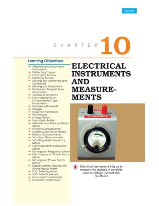
  • 1. ELECTRICAL INSTRUMENTS AND MEASURE- MENTS Learning Objectives ➣ ➣ ➣ ➣ ➣ Absolute and Secondary Instruments ➣ ➣ ➣ ➣ ➣ Deflecting Torque ➣ ➣ ➣ ➣ ➣ Controlling Torque ➣ ➣ ➣ ➣ ➣ Damping Torque ➣ ➣ ➣ ➣ ➣ Moving-iron Ammeters and Voltmeters ➣ ➣ ➣ ➣ ➣ Moving-coil Instruments ➣ ➣ ➣ ➣ ➣ Permanent Magnet Type Instruments ➣ ➣ ➣ ➣ ➣ Voltmeter Sensitivity ➣ ➣ ➣ ➣ ➣ Electrodynamic or Dynamometer Type Instruments ➣ ➣ ➣ ➣ ➣ Hot-wire Instruments ➣ ➣ ➣ ➣ ➣ Megger ➣ ➣ ➣ ➣ ➣ Induction Voltmeter ➣ ➣ ➣ ➣ ➣ Wattmeters ➣ ➣ ➣ ➣ ➣ Energy Meters ➣ ➣ ➣ ➣ ➣ Electrolytic Meter ➣ ➣ ➣ ➣ ➣ Ampere-hour Mercury Motor Meter ➣ ➣ ➣ ➣ ➣ Friction Compensation ➣ ➣ ➣ ➣ ➣ Commutator Motor Meters ➣ ➣ ➣ ➣ ➣ Ballistic Galvanometer ➣ ➣ ➣ ➣ ➣ Vibration Galvanometer ➣ ➣ ➣ ➣ ➣ Vibrating-reed Frequency Meter ➣ ➣ ➣ ➣ ➣ Electrodynamic Frequency Meter ➣ ➣ ➣ ➣ ➣ Moving-iron Frequency Meter ➣ ➣ ➣ ➣ ➣ Electrodynamic Power Factor Meter ➣ ➣ ➣ ➣ ➣ Moving-iron Power Factor Meter ➣ ➣ ➣ ➣ ➣ Nalder-Lipman Moving-iron Power Factor Meter ➣ ➣ ➣ ➣ ➣ D.C. Potentiometer ➣ ➣ ➣ ➣ ➣ A.C. Potentiometers ➣ ➣ ➣ ➣ ➣ Instrument Transformers ➣ ➣ ➣ ➣ ➣ Potential Transformers. Electrical instruments help us to measure the changes in variables such as voltage, current and resistance © 10 C H A P T E R
  • 2. 376 ElectricalTechnology 10.1. Absolute and Secondary Instruments The various electrical instruments may, in a very broad sense, be divided into (i) absolute instruments and (ii) secondary instruments. Absolute instruments are those which give the value of the quantity to be measured, in terms of the constants of the instrument and their deflection only. No previous calibration or comparision is necessary in their case. The example of such an instrument is tangent galvanometer, which gives the value of current, in terms of the tangent of deflection produced by the current, the radius and number of turns of wire used and the horizontal component of earth’s field. Secondary instruments are those, in which the value of electrical quantity to be measured can be determined from the deflection of the instruments, only when they have been pre- calibrated by comparison with an absolute instrument. Without calibration, the deflection of such instruments is meaningless. It is the secondary instruments, which are most generally used in everyday work; the use of the absolute instruments being merely confined within laboratories, as standardizing instruments. 10.2. Electrical Principles of Operation All electrical measuring instruments depend for their action on one of the many physical effects of an electric current or potential and are generally classified according to which of these effects is utilized in their operation. The effects generally utilized are : 1. Magnetic effect - for ammeters and voltmeters usually. 2. Electrodynamic effect - for ammeters and voltmeters usually. 3. Electromagnetic effect - for ammeters, voltmeters, wattmeters and watthour meters. 4. Thermal effect - for ammeters and voltmeters. 5. Chemical effect - for d.c. ampere-hour meters. 6. Electrostatic effect - for voltmeters only. Another way to classify secondary instruments is to divide them into (i) indicating instruments (ii) recording instruments and (iii) integrating instruments. Indicating instruments are those which indicate the instantaneous value of the electrical quantity being measured at the time at which it is being measured. Their indications are given by pointers moving over calibrated dials. Ordinary ammeters, voltmeters and wattmeters belong to this class. Recording instruments are those, which, instead of indicating by means of a pointer and a scale the instantaneous value of an electrical quantity, give a continuous record or the variations of such a quantity over a selected period of time. The moving system of the instrument carries an inked pen which rests lightly on a chart or graph, that is moved at a uniform and low speed, in a direction perpendicular to that of the deflection of the pen. The path traced out by the pen presents a continu- ous record of the variations in the deflection of the instrument. Integrating instruments are those which measure and register by a set of dials and pointers either the total quantity of electricity (in amp-hours) or the total amount of electrical energy (in watt-hours or kWh) supplied to a circuit in a given time. This summation gives the product of time and the electrical quantity but gives no direct indication as to the rate at which the quantity or energy is being supplied because their registrations are independent of this rate provided the current flowing through the instrument is sufficient to operate it. Ampere-hour and watt-hour meters fall in this class. An absolute instrument
  • 3. Electrical Instruments and Measurements 377 10.3. Essentials of Indicating Instruments As defined above, indicating instruments are those which indicate the value of the quantity that is being measured at the time at which it is measured. Such instruments consist essentially of a pointer which moves over a calibrated scale and which is attached to a moving system pivoted in jewelled bearings. The moving system is subjected to the following three torques : 1. A deflecting (or operating) torque 2. A controlling (or restoring) torque 3. A damping torque. 10.4. Deflecting Torque The deflecting or operating torque (Td) is produced by utilizing one or other effects mentioned in Art. 10.2 i.e. magnetic, electrostatic, electrodynamic, thermal or inductive etc. The actual method of torque production depends on the type of instrument and will be discussed in the succeeding para- graphs. This deflecting torque causes the moving system (and hence the pointer attached to it) to move from its ‘zero’ position i.e. its position when the instrument is disconnected from the supply. 10.5. Controlling Torque The deflection of the moving system would be indefinite if there were no controlling or restoring torque. This torque oppose the deflecting torque and increases with the deflection of the moving system. The pointer is brought to rest at a position where the two opposing torques are equal. The deflecting torque ensures that currents of different magnitudes shall produce deflections of the mov- ing system in proportion to their size. Without such at torque, the pointer would swing over to the maximum deflected position irrespective of the magnitude of the current to be measured. Moreover, in the absence of a restoring torque, the pointer once deflected, would not return to its zero position on removing the current. The controlling or restoring or balancing torque in indicating instruments is obtained either by a spring or by gravity as described below : (a) Spring Control A hair-spring, usually of phosphor- bronze, is attached to the moving system of the instrument as shown in Fig. 10.1 (a). With the deflection of the pointer, the spring is twisted in the opposite direction. This twist in the spring produces restoring torque which is directly proportional to the angle of deflection of the moving system. The pointer comes to a position of rest (or equilibrium) when the deflecting torque (Td) and controlling torque (Tc) are equal. For example, in permanent-magnet, moving-coil type of instruments, the deflecting torque is proportional to the current passing through them. ∴ Td ∝I and for spring control Tc ∝θ As Tc = Td ∴ θ ∝ I Fig. 10.1
  • 4. 378 ElectricalTechnology Since deflection θ is directly proportional to current I, the spring-controlled instruments have a uniform or equally-spaced scales over the whole of their range as shown in Fig. 10.1 (b). To ensure that controlling torque is proportional to the angle of deflection, the spring should have a fairly large number of turns so that angular deformation per unit length, on full-scale deflec- tion, is small. Moreover, the stress in the spring should be restricted to such a value that it does not produce a permanent set in it. Springs are made of such materials which (i) are non-magnetic (ii) are not subject to much fatigue (iii) have low specific resistance-especially in cases where they are used for leading current in or out of the instrument (iv) have low temperature-resistance coefficient. The exact expression for controlling torque is Tc = Cθ where C is spring constant. Its value is given by C = 3 Ebt L N-m/rad. The angle θ is in radians. (b) Gravity Control Gravity control is obtained by attaching a small adjustable weight to some part of the moving system such that the two exert torques in the opposite directions. The usual arrangements is shown in Fig. 10. 2(a). It is seen from Fig. 10.2 (b) that the con- trolling or restoring torque is proportional to the sine of the angle of deflection i.e. Tc ∝sin θ The degree of control is adjusted by screwing the weight up or down the carry- ing system It Td ∝ I then for position of rest Td = Tc or I ∝ sin θ (not θ) It will be seen from Fig. 10.2 (b) that as θ approaches 90º, the distance AB increases by a relatively small amount for a given change in the angle than when θ is just increasing from its zero value. Hence, gravity-controlled instruments have scales which are not uniform but are cramped or crowded at their lower ends as shown in Fig. 10.3. As compared to spring control, the disadvantages of gravity control are : 1. it gives cramped scale 2. the instrument has to be kept vertical. However, gravity control has the following advantages : 1. it is cheap 2. it is unaffected by temperature 3. it is not subjected to fatigue or deterioration with time. Example 10.1 The torque of an ammeter varies as the square of the current through it. If a current of 5 A produces a deflection of 90º, what deflection will occur for a current of 3 A when the instrument is (i) spring-controlled and (ii) gravity-controlled. (Elect. Meas. Inst and Meas. Jadavpur Univ.) Fig. 10.2 Fig. 10.3
  • 5. Electrical Instruments and Measurements 379 Solution. Since deflecting torque varies as (current) 2 , we have Td ∝I 2 For spring control, Tc ∝ θ ∴ θ ∝ I 2 For gravity control, Tc ∝sin θ ∴ sin θ ∝ I2 (i) For spring control 90º ∝5 2 and θ ∝3 2 ; θ = 90° × 3 2 /5 2 = 32.4º (ii) For gravity control sin 90º ∝5 2 and sin θ ∝3 2 sin θ = 9/25 = 0.36 ; θ = sin− 1 (0.36) = 21.1º. 10.6. Damping Torque A damping force is one which acts on the moving system of the instrument only when it is moving and always opposes its motion. Such stabilizing or demping force is necessary to bring the pointer to rest quickly, otherwise due to inertia of the moving system, the pointer will oscillate about its final deflected position for quite some time before coming to rest in the steady position. The degree of damping should be adjusted to a value which is sufficient to enable the pointer to rise quickly to its deflected position without overshooting. In that case, the instrument is said to be dead-beat. Any increase of damping above this limit i.e. overdamping will make the instruments slow and lethargic. In Fig. 10.4 is shown the effect of damping on the variation of position with time of the moving system of an instrument. The damping force can be produced by (i) air frictions (ii) eddy currents and (iii) fluid friction (used occasionally). Two methods of air-friction damping are shown in Fig. 10.5 (a) and 10.5 (b). In Fig.. 10.5 (a), the light aluminium piston attached to the moving system of the instrument is arranged to travel with Fig. 10.5 a very small clearance in a fixed air chamber closed at one end. The cross-section of the chamber is either circular or rectangular. Damping of the oscillation is affected by the compression and suction actions of the piston on the air enclosed in the chamber. Such a system of damping is not much favoured these days, those shown in Fig. 10.5 (b) and (c) being preferred. In the latter method, one or two light aluminium vanes are mounted on the spindle of the moving system which move in a closed sector-shaped box as shown. Fluid-friction is similar in action to the air friction. Due to greater viscosity of oil, the damping is more effective. However, oil damping is not much used because of several disadvantages such as objectionable creeping of oil, the necessity of using the instrument always in the vertical position and its obvious unsuitability for use in portable instruments. Fig. 10.4 Piston V Air Chamber Control Spring Vanes Sector Shaped Box Vane (a) (b) (c)
  • 6. 380 ElectricalTechnology The eddy-current form of damping is the most efficient of the three. The two forms of such a damping are shown in Fig. 10.6 and 10.7. In Fig. 10.6 (a) is shown a thin disc of a conducting but non-magnetic material like copper or aluminium mounted on the spindle which carries the moving system and the pointer of the instrument. The disc is so positioned that its edges, when in rotation, cut the magnetic flux between the poles of a permanent magnet. Hence, eddy currents are produced in the disc which flow and so produce a damping force in such a direction as to oppose the very cause producing them (Lenz’s Law Art. 7.5). Since the cause producing them is the rotation of the disc, these eddy current retard the motion of the disc and the moving system as a whole. Fig. 10.6 In Fig. 10.7 is shown the second type of eddy-current damping generally employed in permanent-magnet moving coil instru- ments. The coil is wound on a thin light aluminium former in which eddy currents are produced when the coil moves in the field of the permanent magnet. The direc- tions of the induced currents and of the damping force produced by them are shown in the figure. The various types of instruments and the order in which they would be discussed in this chapter are given below. Ammeters and voltmeters 1. Moving-iron type (both for D.C./A.C.) (a) the attraction type (b) the repulsion type 2. Moving-coil type (a) permanent-magnet type (for D.C. only) (b) electrodynamic or dynamometer type (for D.C./A.C.) 3. Hot-wire type (both for D.C./A.C.) 4. Induction type (for A.C. only) (a) Split-phase type (b) Shaded-pole type 5. Electrostatic type-for voltmeters only (for D.C./A.C.) Fig. 10.7
  • 7. Electrical Instruments and Measurements 381 Wattmeter 6. Dynamometer type (both for D.C./A.C.), 7. Induction type (for A.C. only) 8. Electrostatic type (for D.C. only) Energy Meters 9. Electrolytic type (for D.C. only) 10. Motor Meters (i) Mercury Motor Meter. For d.c. work only. Can be used as amp-hour or watt-hour meter. (ii) Commutator Motor Meter. Used on D.C./A.C. Can be used as Ah or Wh meter. (iii) Induction type. For A.C. only. 11. Clock meters (as Wh-meters). 10.7. Moving-iron Ammeters and Voltmeters There are two basic forms of these instruments i.e. the attraction type and the repulsion type. The operation of the attraction type depends on the at- traction of a single piece of soft iron into a magnetic field and that of repul- sion type depends on the repulsion of two adjacent pieces of iron magnetised by the same magnetic field. For both types of these instruments, the neces- sary magnetic field is produced by the ampere-turns of a current-carrying coil. In case the instrument is to be used as an ammeter, the coil has comparatively fewer turns of thick wire so that the ammeter has low resis- tance because it is connected in series with the circuit. In case it is to be used as a voltmeter, the coil has high impedance so as to draw as small a current as possible since it is connected in par- allel with the circuit. As the current through the coil is small, it has large number of turns in order to produce sufficient ampere-turns. 10.8. Attraction Type M.I. Insturments The basic working principle of an attrac- tion-type moving-iron instrument is illustrated in Fig. 10.8. It is well-known that if a piece of an unmagnetised soft iron is brought up near either of the two ends of a current-carrying coil, it would be attracted into the coil in the same way as it would be attracted by the pole of a bar magnet. Hence, if we pivot an oval-shaped disc of soft iron on a spindle between bear- ings near the coil (Fig. 10.8), the iron disc will swing into the coil when the latter has an elec- tric current passing through it. As the field strength would be strongest at the centre of Fig. 10.8 Moving iron ammeter Moving iron voltmeter
  • 8. 382 ElectricalTechnology the coil, the ovalshaped iron disc is pivoted in such a way that the greatest bulk of iron moves into the centre of the coil. If a pointer is fixed to the spindle carrying the disc, then the passage of current through the coil will cause the pointer to deflect. The amount of deflection produced would be greater when the current producing the magnetic field is greater. Another point worth noting is that whatever the direction of current through the coil, the iron disc would always be magnetised in such a way that it is pulled inwards. Hence, such instruments can be used both for direct as well as alternating currents. A sectional view of the actual instrument is shown in Fig. 10.9. When the current to be measured is passed through the coil or solenoid, a magnetic field is produced, which attracts the eccentrically- mounted disc inwards, thereby deflecting the pointer, which moves over a calibrated scale. Deflecting Torque Let the axis of the iron disc, when in zero position, subtend an angle of φwith a direction perpen- dicular to the direction of the field H produced by the coil. Let the deflection produced be θ corre- sponding to a current I through the coil. The magnetisation of iron disc is proportional to the compo- nent of H acting along the axis of the disc i.e. proportional to H cos [90 −(φ + θ)] or H sin (θ + φ). The force F pulling the disc inwards is proportional to MH or H 2 sin (θ + φ). If the permeability of iron is assumed constant, then, H ∝I. Hence, F ∝I 2 sin (θ + φ). If this force acted at a distance of l from the pivot of the rotating disc, then deflecting torque Td = Fl cos (θ + φ). Putting the value of F, we get Td ∝I 2 sin (θ + φ) × l cos (θ + φ) ∝I 2 sin 2 (θ + φ) = KI 2 sin 2 (θ + φ) ...sin l is constant If spring-control is used, then controlling torque Tc = K′ θ In the steady position of deflection, Td = Tc ∴ KI 2 sin 2 (θ + φ) = K′ θ ; Hence θ∝ I 2 Fig. 10.9 Fig. 10.10 If A.C. is used, then θ ∝ I2 r.m.s. However, if gravity-control is used, then Tc = K1 sin θ ∴ KI 2 sin 2 (θ + φ) = K1 sin θ ∴ sin θ αI 2 sin 2 (θ + φ) In both cases, the scales would be uneven. Damping As shown, air-friction damping is provided, the actual arrangement being a light piston moving in an air-chamber. 10.9. Repulsion Type M.I. Instruments The sectional view and cut-away view of such an instrument are shown in Fig. 10.11 and 10.12. It consists of a fixed coil inside which are placed two soft-iron rods (or bars) A and B parallel to one another and along the axis of the coil. One of them i.e. A is fixed and the other B which is movable carries a pointer that moves over a calibrated scale. When the current to be measured is passed
  • 9. Electrical Instruments and Measurements 383 Fig. 10.11 Fig. 10.12 through the fixed coil, it sets up its own magnetic field which magnetises the two rods similarly i.e. the adjacent points on the lengths of the rods will have the same magnetic polarity. Hence, they repel each other with the result that the pointer is deflected against the controlling torque of a spring or gravity. The force of repulsion is approximately proportional to the square of the current passing through the coil. Moreover, whatever may be the direction of the current through the coil, the two rods will be magnetised similaraly and hence will repel each other. In order to achieve uniformity of scale, two tongue-shaped strips of iron are used instead of two rods. As shown in Fig. 10.13 (a), the fixed iron consists of a tongue-shaped sheet iron bent into a cylindrical form, the moving iron also consists of another sheet of iron and is so mounted as to move parallel to the fixed iron and towards its narrower end [Fig. 10.13 (b)]. Deflecting Torque The deflecting torque is due to the repulsive force between the two similarly magnetised iron rods or sheets. Fig. 10.13 Instantaneous torque ∝repulsive force ∝m1m2 ...product of pole strengths Since pole strength are proportional to the magnetising force H of the coil, ∴ instantaneous torque ∝H 2 Since H itself is proportional to current (assuming constant permeability) passing through the coil, ∴ instantaneous torque ∝ I 2 Hence, the deflecting torque, which is proportional to the mean torque is, in effect, proportional to the mean value of I2 . Therefore, when used on a.c. circuits, the instrument reads the r.m.s. value of current. Scales of such instruments are uneven if rods are used and uniform if suitable-shaped pieces of iron sheet are used. The instrument is either gravity-controlled or as in modern makes, is spring-controlled. Damping is pneumatic, eddy current damping cannot be employed because the presence of a permanent magnet required for such a purpose would affect the deflection and hence, the reading of the instrument. Since the polarity of both iron rods reverses simultaneously, the instrument can be used both for a.c. and d.c. circuits i.e. instrument belongs to the unpolarised class.
  • 10. 384 ElectricalTechnology 10.10. Sources of Error There are two types of possible errors in such instruments, firstly, those which occur both in a.c. and d.c. work and secondly, those which occur in a.c. work alone. (a) Errors with both d.c. and a.c. work (i) Error due to hysteresis. Because of hysteresis in the iron parts of the moving system, read- ings are higher for descending values but lower for ascending values. The hysteresis error is almost completely eliminated by using Mumetal or Perm-alloy, which have negligible hysteresis loss. (ii) Error due to stray fields. Unless shielded effectively from the effects of stray external fields, it will give wrong readings. Magnetic shielding of the working parts is obtained by using a covering case of cast-rion. (b) Errors with a.c. work only Changes of frequency produce (i) change in the impedance of the coil and (ii) change in the magnitude of the eddy currents. The increase in impedance of the coil with increase in the frequency of the alternating current is of importance in voltmeters (Ex. 10.2). For frequencies higher than the one used for calibration, the instrument gives lower values. However, this error can be removed by connecting a capacitor of suitable value in parallel with the swamp resistance R of the instrument. It can be shown that the impedance of the whole circuit of the instrument becomes independent of frequency if C = L/R2 where C is the capacitance of the capacitor. 10.11. Advantages and Disadvantages Such instruments are cheap and robust, give a reliable service and can be used both on a.c. and d.c. circuits, although they cannot be calibrated with a high degree of precision with d.c. on account of the effect of hysteresis in the iron rods or vanes. Hence, they are usually calibrated by comparison with an alternating current standard. 10.12. Deflecting Torque in terms of Change in Self-induction The value of the deflecting torque of a moving-iron instrument can be found in terms of the variation of the self-inductance of its coil with deflection θ. Suppose that when a direct current of I passes through the instrument, its deflection is θ and inductance L. Further suppose that when current changes from I to (I + dI), deflection changes from θ to (θ + dθ) and L changes to (L + dL). Then, the increase in the energy stored in the magnetic field is dE = d ( 1 2 LI 2 ) = 1 2 L2I.dI + 1 2 I 2 dL = LI. dI + 1 2 I 2 . dL joule. If T 1 2 N-m is the controlling torque for deflection θ, then extra energy stored in the control system is T × dθ joules. Hence, the total increase in the stored energy of the system is LI.dI + 1 2 I2 . dL + T × d θ ...(i) The e.m.f. induced in the coil of the instrument is e = N. d dt Φ volt where dφ = change in flux linked with the coil due to change in the posi- tion of the disc or the bars dt = time taken for the above change ; N = No. of turns in the coil Now L = NF/I ∴ Φ = LI/N ∴ 1 . d d dt N dt Φ = (LI) Induced e.m.f. e = N. 1 . d N dt (LI) = d dt (LI) The energy drawn from the supply to overcome this back e.m.f is = e.Idt = d dt (LI).Idt = I.d(LI) = I(L.dI + I.dL) = LI.dI + I 2 .dL ...(ii)
  • 11. Electrical Instruments and Measurements 385 Equating (i) and (ii) above, we get LI.dI + 1 2 I2 dL + T.dθ = LI.dI + I2 .dL ∴ T = 1 2 I2 dL dθ N-m where dL/dθ is henry/radian and I in amperes. 10.13. Extension of Range by Shunts and Multipliers (i) As Ammeter. The range of the moving-iron instrument, when used as an ammeter, can be extended by using a suitable shunt across its terminals. So far as the operation with direct current is concerned, there is no trouble, but with alternating current, the division of current between the instrument and shunt changes with the change in the applied frequency. For a.c. work, both the inductance and resistance of the instrument and shunt have to be taken into account. Obviously, current through instruments, current through shunt, s s s R j L i I R j L + ω = = + ω s Z Z where R, L = resistance and inductance of the instrument Rs, Ls = resistance and inductance of the shunt It can be shown that above ratio i.e. the division of current between the instrument and shunt would be independent of frequency if the time-constants of the instrument coil and shunt are the same i.e. if L/R = Ls/Rs. The multiplying power (N) of the shunt is given by N = 1 s I R i R = + where I = line current ; i = full-scale deflection current of the instrument. (ii) As Voltmeter. The range of this instrument, when used as a voltmeter, can be extended or multiplied by using a high non-inductive resistance R connected in series with it, as shown in Fig. 10.14. This series resistance is known as ‘multiplier’when used on d.c. circuits. Suppose, the range of the instrument is to be extended from ν to V. Then obviously, the excess voltage of (V −ν) is to be dropped across R. If i is the full-scale deflection current of the instrument, then Fig. 10.14 Fig. 10.15 iR = V −ν; R = V ir V V r i i i − − ν = = − Voltage magnification = V/ν. Since iR = V −ν; ∴ 1 iR V = − ν ν or 1 iR V ir = − ν ∴ ( ) 1 V R r = + ν Hence, greater the value of R, greater is the extension in the voltage range of the instrument. For d.c. work, the principal requirement of R is that its value should remain constant i.e. it should have low temperature-coefficient. But for a.c. work it is essential that total impedance of the voltme- ter and the series resistance R should remain as nearly constant as possible at different frequencies. That is why R is made as non-inductive as possible in order to keep the inductance of the whole circuit to the minimum. The frequency error introduced by the inductance of the instrument coil can be compensated by shunting R by a capacitor C as shown in Fig. 10.15. In case r ^ R, the impedance of the voltmeter circuit will remain practically constant (for frequencies upto 1000 Hz) provided.
  • 12. 386 ElectricalTechnology C = 2 2 0.41 (1 2) L L R R = + Example 10.2. A 250-volt moving-iron voltmeter takes a current of 0.05 A when connected to a 250-volt d.c. supply. The coil has an inductance of 1 henry. Determine the reading on the meter when connected to a 250-volt, 100-Hz a.c. supply. (Elect. Engg., Kerala Univ.) Solution. When used on d.c. supply, the instrument offers ohmic resistance only. Hence, resis- tance of the instrument = 250/0.05 = 5000 Ω. When used on a.c. supply, the instrument offers impedance instead of ohmic resistance. impedance at 100 Hz = 2 2 5000 (2 100 1) + π × × = 5039.3 Ω ∴ voltage of the instrument = 250 × 5000/5039.3 = 248 V Example 10.3. A spring-controlled moving-iron voltmeter reads correctly on 250-V d.c. Calcu- late the scale reading when 250-V a.c. is applied at 50 Hz. The instrument coil has a resistance of 500 Ωand an inductance of 1 H and the series (non-reactive) resistance is 2000 Ω. (Elect. Instru. & Measure. Nagpur Univ. 1992) Solution. Total circuit resistance of the voltmeter is = (r + R) = 500 + 2,000 = 2,500 Ω Since the voltmeter reads correctly on direct current supply, its full-scale deflection current is = 250/2500 = 0.1 A. When used on a.c. supply, instrument offers an impedance 2 2 2500 (2 50 1) Z = + π × × = 2.520 Ω ∴ I = 0.099 A ∴ Voltmeter reading on a.c. supply = 250 × 0.099/0.1 = 248 V* Note. Since swamp resistance R = 2,000 Ω, capacitor required for compensating the frequency error is C = 0.41 L/R 2 = 0.41 × 1/2000 2 = 0.1 μF. Example 10.4. A 150-V moving-iron voltmeter intended for 50 Hz has an inductance of 0.7 H and a resistance of 3 kΩ. Find the series resistance required to extend the range of the instrument to 300 V. If this 300-V, 50-Hz instrument is used to measure a d.c. voltage, find the d.c. voltage when the scale reading is 200 V. (Elect. Measur, A.M.I.E. Sec B, 1991) Solution. Voltmeter reactance = 2π × 50 × 0.7 = 220 Ω Impedance of voltmeter = (3000 + j 220) = 3008 Ω When the voltmeter range is doubled, its impedance has also to be doubled in order to have the same current for full-scale deflection. If R is the required series resistance, then (3000 + R)2 + 2202 = (2 × 3008)2 ∴ R = 3012 Ω When used on d.c. supply, if the voltmeter reads 200 V, the actual applied d.c. voltage would be = 200 × (Total A.C. Impedance)/total d.c. resistance) = 200 × (2 × 3008)/(3000 + 3012) = 200 × (6016 × 6012) = 200.134 V. Example 10.5. The coil of a moving-iron voltmeter has a resistance of 5,000 Ωat 15ºC at which temperature it reads correctly when connected to a supply of 200 V. If the coil is wound with wire whose temperature coefficient at 15ºC is 0.004, find the percentage error in the reading when the temperature is 50ºC. In the above instrument, the coil is replaced by one of 2,000 Ωbut having the same number of turns and the full 5,000 Ωresistance is obtained by connecting in series a 3,000 Ωresistor of negli- gible temperature-coefficient. If this instrument reads correctly at 15ºC, what will be its percentage error at 50ºC. Solution. Current at 15ºC = 200/5,000 = 0.04 A Resistance at 50ºC is R50 = R15 (1+ α15 × 35) ∴ R50 = 5,000 (1 + 35 × 0.004) = 5,700 Ω * or reading = 250 × 2500/2520 = 248 V.
  • 13. Electrical Instruments and Measurements 387 ∴ current at 50ºC = 200/5,700 ∴ reading at 50ºC = 200 (200/5,700) 0.04 × = 175.4 V or = 200 × 5000/5700 = 175.4 V ∴ % error = 175.4 200 100 200 − × = − − − − − 12.3% In the second case, swamp resistance is 3,000 Ωwhereas the resistance of the instrument is only 2,000 Ω. Instrument resistance at 50ºC = 2,000 (1 + 35 × 0.004) = 2,280 Ω ∴ total resistance at 50ºC = 3,000 + 2,280 = 5,280 Ω ∴ current at 50ºC = 200/5,280 A ∴ instrument reading = 200 × 200/5,280 0.04 = 189.3 V ∴ percentage error = 189.3 200 100 200 − × = − − − − − 5.4 % Example 10.6. The change of inductance for a moving-iron ammeter is 2μH/degree. The control spring constant is 5 × 10 − 7 N-m/degree. The maximum deflection of the pointer is 100º, what is the current corresponding to maximum deflection ? (Measurement & Instrumentation Nagpur Univ. 1993) Solution. As seen from Art. 10.12 the deflecting torque is given by Td = 2 1 2 dL I dθ N-m Control spring constant = 5 × 10− 7 N-m/degree Deflection torque for 100° deflection = 5 × 10− 7 × 100 = 5 × 10− 5 N-m ; dL/dθ = 2 μH/degree = 2 × 10− 6 H/degree. ∴ 5 × 10 − 5 = 1 2 I 2 × 2 × 10 − 6 ∴ I 2 = 50 and I = 7.07 A Example 10.7. The inductance of attraction type instrument is given by L = (10 + 5θ − θ 2 )μH where θ is the deflection in radian from zero position. The spring constant is 12 × 10 − 6 N-m/rad. Find out the deflection for a current of 5 A. (Elect. and Electronics Measurements and Measuring Instruments Nagpur Univ. 1993) Solution. L = (10 + 5 θ − θ 2 ) × 10 − 6 H ∴ dL dθ = (0 + 5 −2 × θ) × 10–6 = (5 −2θ) × 10− 6 H/rad Let the deflection be θ radians for a current of 5A, then deflecting torque, Td = 12 × 10 − 6 × θ N-m Also, Td = 2 1 2 dL I dθ ...Art. Equating the two torques, we get 12 × 10 − 6 × θ = 1 2 × 5 2 × (5 −2θ) × 10 − 6 ∴ θ = 1.689 radian Tutorial Problems No. 10.1 1. Derive an expression for the torque of a moving-iron ammeter. The inductance of a certain moving- iron ammeter is (8 + 4θ − ½ θ 2 ) μH where θ is the deflection in radians from the zero position. The control- spring torque is 12 × 10 − 6 N-m/rad. Calaculate the scale position in radians for a current of 3A. [1.09 rad] (I.E.E. London) 2. An a.c. voltmeter with a maximum scale reading of 50-V has a resistance of 500 Ωand an inductance of 0.09 henry, The magnetising coil is wound with 50 turns of copper wire and the remainder of the circuit is a non-inductive resistance in series with it. What additional apparatus is needed to make this instrument read correctly on both d.c. circuits or frequency 60 ? [0.44 μF in parallel with series resistance]
  • 14. 388 ElectricalTechnology 3. A 10-V moving-iron ammeter has a full-scale deflection of 40 mA on d.c. circuit. It reads 0.8% low on 50 Hz a.c. Hence, calculate the inductance of the ammeter. [115.5 mH] 4. It is proposed to use a non-inductive shunt to increase the range of a 10-A moving iron ammeter to 100 A. The resistance of the instrument, including the leads to the shunt, is 0.06 Ωand the inductance is 15 μH at full scale. If the combination is correct on a.d.c circuit, find the error at full scale on a 50 Hz a.c. circuit. [3.5 %](London Univ.) 10.14. Moving-coil Instruments There are two types of such instruments (i) permanent-magnet type which can be used for d.c. work only and (ii) the dynamometer type which can be used both for a.c. and d.c. work. 10.15. Permanent Magnet Type Instruments The operation of a permanent-magnet moving-coil type instrument is be based upon the prin- ciple that when a current-carrying conductor is placed in a magnetic field, it is acted upon by a force which tends to move it to one side and out of the field. Construction As its name indicates, the instrument consists of a permanent magnet and a rectangular coil of many turns wound on a light aluminium or copper former inside which is an iron core as shown in Fig. 10.16. Fig. 10.17 Fig. 10.16. The powerfull U-shaped permanent magnet is made of Alnico and has soft-iron end-pole pieces which are bored out cylindrically. Between the magnetic poles is fixed a soft iron cylinder whose function is (i) to make the field radial and uniform and (ii) to decrease the reluctance of the air path between the poles and hence increase the magnetic flux. Surrounding the core is a rectangular coil of many turns wound on a light aluminium frame which is supported by delicate bearings and to which is attached a light pointer. The aluminium frame not only provides support for the coil but also provides damping by eddy currents induced in it. The sides of the coil are free to move in the two air- gaps between the poles and core as shown in Fig. 10.16 and Fig. 10.17. Control of the coil movement is affected by two phosphor-bronze hair springs, one above and one below, which additionally serve the purpose of lending the current in and out of the coil. The two springs are spiralled in opposite directions in order to neutralize the effects of temperature changes. Deflecting Torque When current is passed through the coil, force acts upon its both sides which produce a deflecting torque as shown in Fig. 10.18. Let B = flux density in Wb/m 2 l = length or depth of the coil in metre b = breadth of coil in metre Fig. 10.18
  • 15. Electrical Instruments and Measurements 389 N = number of turns in the coil If I ampere is the current passing through the coil, then the magnitude of the force experienced by each of its sides is = BIl newton For N turns, the force on each side of the coil is = NBIl newton ∴ deflecting torque Td = force × perpendicular distance = NBIl × b = NBI(I × b) = NBIA N-m where A is the face area of the coil. It is seen that if B is constant, then Td is proportional to the current passing through the coil i.e. Td ∝I. Such instruments are invariable spring-controlled so that Tc ∝deflection θ. Since at the final deflected position, Td = Tc ∴θ ∝I Hence, such instruments have uniform scales. Damping is electromagnetic i.e. by eddy currents induced in the metal frame over which the coil is wound. Since the frame moves in an intense magnetic field, the induced eddy currents are large and damping is very effective. 10.16. Advantage and Disadvantages The permanent-magnet moving-coil (PMMC) type instruments have the following advantages and disadvantages : Advantages 1. they have low power consumption. 2. their scales are uniform and can be designed to extend over an arc of 170° or so. 3. they possess high (torque/weight) ratio. 4. they can be modified with the help of shunts and resistances to cover a wide range of cur- rents and voltages. 5. they have no hysteresis loss. 6. they have very effective and efficient eddy-current damping. 7. since the operating fields of such instruments are very strong, they are not much affected by stray magnetic fields. Disadvantages 1. due to delicate construction and the necessary accurate machining and assembly of various parts, such instruments are somewhat costlier as compared to moving-iron instruments. 2. some errors are set in due to the aging of control springs and the parmanent magnets. Such instruments are mainly used for d.c. work only, but they have been sometimes used in conjunction with rectifiers or thermo-junctions for a.c. measurements over a wide range or frequencies. Permanent-magnet moving-coil instruments can be used as ammeters (with the help of a low resistance shunt) or as voltmeters (with the help of a high series resistance). The principle of permanent-magnet moving-coil type instruments has been utilized in the construction of the fol- lowing : 1. For a.c. galvanometer which can be used for detect- ing extremely small d.c. currents. A galvanometer may be used either as an ammeter (with the help of a low resistance) or as a voltmeter (with the help of a high series resistance). Such a galvanometer (of pivoted type) is shown in Fig. 10.19. 2. By eliminating the control springs, the instrument can be used for measuring the quantity of electric- ity passing through the coil. This method is used for fluxmeters. Fig. 10.19
  • 16. 390 ElectricalTechnology 3. If the control springs of such an instrument are purposely made of large moment of inertia, then it can be used as ballistic galvanometer. 10.17. Extension of Range (i) As Ammeter When such an instrument is used as an ammeter, its range can be extended with the help of a low- resistance shunt as shown in Fig. 10.12 (a). This shunt provides a bypath for extra current because it is connected across (i.e. in parallel with) the instrument. These shunted instruments can be made to record currents many times greater than their normal full-scale de- flection currents. The ratio of maximum current (with shunt) to the full-scale deflection current (without shunt) is known as the ‘multi- plying power’ or ‘multiplying factor’ of the shunt. Let Rm = instrument resistance S = shunt resistance Im = full-scale deflection current of the instrument I = line current to be measured As seen from Fig. 10.20 (a), the voltage across the instrument coil and the shunt is the same since both are joined in parallel. ∴ Im × Rm = S Is = S (I −Im) ∴ S = ( ) m m m I R I I − ; Also 1 m m R I I S ⎛ ⎞ = + ⎜ ⎟ ⎝ ⎠ ∴ multiplying power = 1 m R S ⎛ ⎞ + ⎜ ⎟ ⎝ ⎠ Obviously, lower the value of shunt resistance, greater its multiplying power. (ii) As voltmeter The range of this instrument when used as a voltmeter can be increased by using a high resistance in series with it [Fig. 10.20 (b)]. Let Im = full-scale deflection current Rm = galvanometer resistance ν = RmIm = full-scale p.d. across it V = voltage to be measured R = series resistance required Then it is seen that the voltage drop across R is V −ν ∴ R = m V I − ν or R . Im = V −ν Dividing both sides by ν, we get m RI ν = 1 V − ν or . 1 1 m m m m R I V V R I R R ⎛ ⎞ = − ∴ = + ⎜ ⎟ ν ν ⎝ ⎠ ∴ voltage multiplication = 1 m R R ⎛ ⎞ + ⎜ ⎟ ⎝ ⎠ Obviously, larger the value of R, greater the voltage multiplication or range. Fig. 10.20 (b) shown a voltmeter with a single multiplier resistor for one range. A multi-range voltmeter requires on multiplier resistor for each additional range. Example 10.8. A moving coil ammeter has a fixed shunt of 0.02 Ωwith a coil circuit rtesistance of R = 1 kΩand need potential difference of 0.5 V across it for full-scale deflection. (1) To what total current does this correspond ? (2) Calculate the value of shunt to give full scale deflection when the total current is 10 A and 75 A. (Measurement & Instrumentation Nagpur Univ. 1993) Fig. 10.20 (a) Fig. 10.20 (b)
  • 17. Electrical Instruments and Measurements 391 Fig. 10.21 Solution. It should be noted that the shunt and the meter coil are in parallel and have a common p.d. of 0.5 V applied across them. (1) ∴Im = 0.5/1000 = 0.0005 A; Is = 0.5./0.02 = 25 A ∴ line current = 25.0005 A (2) When total current is 10 A, Is = (10 −0.0005) = 9.9995 A ∴ S = 0.0005 1000 9.9995 m m s I R I × = = 0.05 Ω When total current is 75 A, Is = (75− 0.0005) = 74.9995 A ∴ S = 0.0005 × 1000/74.9995 = 0.00667 Ω Ω Ω Ω Ω Example 10.9. A moving-coil instrument has a resistance of 10 Ωand gives full-scale deflec- tion when carrying a current of 50 mA. Show how it can be adopted to measure voltage up to 750 V and currents upto 1000 A. (Elements of Elect. Engg.I, Bangalore Univ.) Solution. (a) As Ammeter. As discussed above, current range of the meter can be extended by us- ing a shunt across it [Fig. 10.21 (a)]. Obviously, 10 × 0.05 = S × 99.95 ∴ S = 0.005 Ω Ω Ω Ω Ω (b) As Voltmeter. In this case, the range can be extended by using a high resistance R in series with it. [Fig. 10.21 (b)]. Obviously, R must drop a voltage of (750− 0.5) = 749.5 V while carrying 0.05A. ∴ 0.05 R = 749.5 or R = 14.990 Ω Ω Ω Ω Ω Example 10.10. How will you use a P.M.M.C. instrument which gives full scale deflection at 50 mV p.d. and 10 mA current as (1) Ammeter 0 - 10 A range (2) Voltmeter 0-250 V range (Elect. Instruments & Measurements Nagpur Univ. 1993) Solution. Resistance of the instrument Rm = 50 mV/10 mA = 5 (i) As Ammeter full-scale meter current, Im = 10 mA = 0.01 A shunt current Is = I −Im = 10 −0.01 = 9.99 A Reqd. shunt resistance, S = . 0.01 5 ( ) 9.99 m m m I R I I × = − = 0.0005 Ω (ii) As Voltmeter Full-scale deflection voltage, ν = 50 mV = 0.05 V; V = 250 V Reqd. series resistance, R = 250 0.05 0.01 m V I − − ν = = 24,995 Ω Example 10.11. A current galvanometer has the following parameters : B = 10 × 10− 3 Wb/m2 ; N = 200 turns, l = 16 mm; d = 16 mm; k = 12 × 10− 9 Nm/radian. Calculate the deflection of the galvanometer when a current of 1 μA flows through it. (Elect. Measurement Nagpur Univ. 1993)
  • 18. 392 ElectricalTechnology Solution. Deflecting torque Td = NBIA N− m = 200 × (10 × 10− 3 ) × (1 × 10− 6 ) × (1 × 10− 3 ) × (16 × 10 − 3 ) N-m = 512 × 10 − 12 N− m Controlling torque Tc = controlling spring constant × deflection = 12 × 10− 9 × θ N− m Equating the deflecting and controlling torques, we have 12 × 110 − 9 × θ = 512 × 10 − 12 ∴ θ = 0.0427 radian = 2.45º Example 10.12. The coil of a moving coil permanent magnet voltmeter is 40 mm long and 30 mm wide and has 100 turns on it. The control spring exerts a torque of 120 × 10 − 6 N-m when the deflection is 100 divisions on full scale. If the flux density of the magnetic field in the air gap is 0.5 Wb/m2 , estimate the resistance that must be put in series with the coil to give one volt per division. The resistance of the voltmeter coil may be neglected. (Elect. Mesur.AMIE Sec. B Summer 1991) Solution. Let I be the current for full-scale deflection. Deflection torque Td = NBIA = 100 × 0.5 × I × (1200 × 10 − 6 ) = 0.06 I N-m Controlling torque Tc = 120 × 10 − 6 N-m In the equilibrium position, the two torques are equal i.e. Td = Tc. ∴ 0.06 I = 120 × 10 − 6 ∴ I = 2 × 10 − 3 A. Since the instrument is meant to read 1 volt per division, its full-scale reading is 100 V. Total resistance = 100/2 × 10 − 3 = 50,000 Ω Since voltmeter coil resistance is negligible, it represents the additional required resistance. Example 10.13. Show that the torque produced in a permanent-magnet moving-coil instrument is proportional to the area of the moving coil. A moving-coil voltmeter gives full-scale deflection with a current of 5 mA. The coil has 100 turns, effective depth of 3 cm and width of 2.5 cm. The controlling torque of the spring is 0.5 cm for full-scale deflection. Estimate the flux density in the gap. (Elect. Meas, Marathwads Univ.) Solution. The full-scale deflecting torque is Td = NBIA N-m where I is the full-scale deflection current ; I = 5 mA = 0.005 A Td = 100 × B × 0.005 × (3 × 2.5 × 10− 4 ) = 3.75 × 10− 4 B N-m The controlling torque is Tc = 0.5 g-cm = 0.5 g. wt.cm = 0.5 × 10− 3 × 10− 2 kg wt-m = 0.5 × 10− 5 × 9.8 = 4.9 × 10− 5 N-m For equilibrium, the two torques are equal and opposite. ∴ 4.9 × 10− 5 = 3.75 × 10− 4 B ∴ B = 0.13 Wb/m2 Example 10.14. A moving-coil milliammeter has a resistance of 5 Ωand a full-scale deflection of 20 mA. Determine the resistance of a shunt to be used so that the instrument could measure currents upto 500 mA at 20° C. What is the percentage error in the instrument operating at a temperature of 40°C ? Temperature co-efficient of copper = 0.0039 per °C. (Measu. & Instrumentation, Allahabad Univ. 1991) Solution. Let R20 be the shunt resistance at 20°C. When the temperature is 20°C, line current is 500 mA and shunt current is = (500− 20) = 480 mA. ∴ 5 × 20 = R20 × 480, R20 = 1/4.8 Ω If R40 is the shunt resistance at 40ºC, then R40 R20 (1 + 20 α) = 1 4.8 (1 + 0.0039 × 20) = 1.078 4.8 Ω Shunt current at 40ºC is = 5 20 1.078/4.8 × = 445 mA Line current = 445 + 20 = 465 mA Although, line current would be only 465 mA, the instrument will indicate 500 mA. ∴ error = 35/500 = 0.07 or 7%
  • 19. Electrical Instruments and Measurements 393 Example 10.15. A moving-coil millivoltmeter has a resistance of 20Ωand full-scale deflection of 120º is reached when a potential difference of 100 mV is applied across its terminals. The moving coil has the effective dimensions of 3.1 cm × 2.6 cm and is wound with 120 turns. The flux density in the gap is 0.15 Wb/m2 . Determine the control constant of the spring and suitable diameter of copper wire for coil winding if 55% of total instrument resistance is due to coil winding. ρ for copper = 1.73 × 10 − 6 Ω cm. (Elect. Inst. and Meas. M.S. Univ. Baroda) Solution. Full-scale deflection current is = 100/20 = 5 mA Deflecting torque for full-scale deflection of 120º is Td = NBIA = 120 × 0.15 × (5 × 10 − 3 ) × (3.1 × 2.6 × 10 − 4 ) = 72.5 × 10 − 6 N-m Control constant is defined as the deflecting torque per radian (or degree) or deflection of mov- ing coil. Since this deflecting torque is for 120° deflection. Control constant = 72.5 × 10 − 6 /120 = 6.04 × × × × × 10− − − − − 7 N-m/degree Now, resistance of copper wire = 55% of 20 Ω= 11 Ω Total length of copper wire = 120 × 2 (3.1 + 2.6) = 1368 cm Now R = ρl/A ∴ A = 1.73 × 10 − 6 × 1368/11 = 215.2 × 10 − 6 cm 2 ∴ π d 2 /4 = 215.2 × 10 − 6 ∴ d = 6 215 4 10 / − × × π = 16.55 × 10− 3 cm = 0.1655 mm 10.18. Voltmeter Sensitivity It is defined in terms of resistance per volt (Ω/V). Suppose a meter movement of 1 kΩinternal resistance has s full-scale deflection current of 50 μ A. Obviously, full-scale voltage drop of the meter movement is = 50 μA × 1000 Ω= 50 mV. When used as a voltmeter, its sensitivity would be 1000/50 × 10 − 3 = 20 kΩ/V. It should be clearly understood that a sensitivity of 20 kΩ/V means that the total resistance of the circuit in which the above movement is used should be 20 kΩfor a full-scale deflection of 1 V. 10.19. Multi-range Voltmeter It is a voltmeter which measures a number of voltage ranges with the help of different series resistances. The resistance required for each range can be easily calculated provided we remember one basic fact that the sensitivity of a meter movement is always the same regardless of the range selected. Moreover, the full-scale deflection current is the same in every range. For any range, the total circuit resistance is found by multiplying the sensitivity by the full-scale voltage for that range. For example, in the case of the above-mentioned 50μA, 1 kΩmeter movement, total resistance required for 1 V full-scale deflection is 20 kΩ. It means that an additional series resistance of 19 kΩ is required for the purpose as shown in Fig. 10.22 (a). Fig. 10.22 For 10-V range, total circuit resistance must be (20 kΩ/V) (10 V) = 200 kΩ. Since total resis- tance for 1 V range is 20 kΩ, the series resistance R for 10-V range = 200 −20 = 180 kΩas shown in Fig. 10.22 (b). For the range of 100 V, total resistance required is (20 kΩ/V) (100 V) = 2 MΩ. The additional resistance required can be found by subtracting the existing two-range resistance from the total
  • 20. 394 ElectricalTechnology resistance of 2 MΩ. Its value is = 2 M Ω− 180 kΩ− 19 kΩ− 1 kΩ = 1.8 MΩ It is shown in Fig. 10.22 (c). Example 10.16. A basic 1’ Arsonval movement with internal resistance Rm = 100 Ω and full scale deflection current If = 1 mA is to be converted into a multirange d.c. voltmeter with voltage ranges of 0− 10 V, 0− 50 V, 0− 250 V and 0− 500 V. Draw the necessary circuit arrangement and find the values of suitable multipliers. (Instrumentation AMIE Sec. B Winter 1991) Solution. Full-scale voltage drop = (1 mA) (100 Ω) = 100 mV. Hence, sensitivity of this move- ment is 100/100 × 10 − 3 = 1 kΩ/V. (i) 0− − − − − 10 V range Total resistance required = (1 kΩ/V) (10 V) = 10 kΩ. Since meter resistance is 1 kΩadditional series resistance required for this range R1 = 10 −1 = 9 kΩ Ω Ω Ω Ω (ii) 0-50 V range RT = (1 kΩ/V) (50 V) = 50 kΩ; R2 = 50− 9− 1 = 40 kΩ Ω Ω Ω Ω (iii) 0− − − − − 250 V range RT = (1 kΩ/V) (250 V) = 250 kΩ; R3 = 250 −50 = 200 kΩ Ω Ω Ω Ω (iv) 0− − − − − 500 V range RT = (1 kΩ/V) (500 V) = 500 kΩ ; R4 = 500 −250 = 250 kΩ Ω Ω Ω Ω The circuit arrangement is similar to the one shown in Fig. 10.22 Tutorial problem No. 10.2 1. The flux density in the gap of a 1-mA (full scale) moving ‘-coil’ ammeter is 0.1 Wb/m2 . The rectan- gular moving-coil is 8 mm wide by 1 cm deep and is wound with 50 turns. Calculate the full-scale torque which must be provided by the springs. [4 × × × × × 10− − − − − 7 N-m] (App. Elec. London Univ.) 2. A moving-coil instrument has 100 turns of wire with a resistance of 10 Ω, an active length in the gap of 3 cm and width of 2 cm. A p.d. of 45 mV produces full-scale deflection. The control spring exerts a torque of 490.5 × 10 − 7 N-m at full-scale deflection. Calculate the flux density in the gap. [0.1817 Wb/m2] (I.E.E. London) 3. A moving-coil instrument, which gives full-scale deflection with 0.015 A has a copper coil having a resistance of 1.5 Ωat 15°C and a temperature coefficient of 1/234.5 at 0°C in series with a swamp resistance of 3.5 Ωhaving a negligible temperature coefficient. Determine (a) the resistance of shunt required for a full-scale deflection of 20 A and (b) the resistance required for a full-scale deflection of 250 V. If the instrument reads correctly at 15°C, determine the percentage error in each case when the temperature is 25°C. [(a) 0.00376 Ω Ω Ω Ω Ω; 1.3 % (b) 16,662 Ω Ω Ω Ω Ω, negligible] (App. Elect. London Univ.) 4. A direct current ammeter and leads have a total resistance of 1.5 Ω. The instrument gives a full-scale deflection for a current of 50 mA. Calculate the resistance of the shunts necessary to give full-scale ranges of 2-5, 5.0 and 25.0 amperes [0.0306 ; l 0.01515 ; 0.00301 Ω Ω Ω Ω Ω] (I.E.E. London) 5. The following data refer to a moving-coil voltmeter : resistance = 10,000 Ω, dimensions of coil = 3 cm × 3 cm ; number of turns on coil = 100, flux density in air-gap = 0.08 Wb/m2 , stiffness of springs = 3 × 10− 6 N-m per degree. Find the deflection produced by 110 V. [48.2º] (London Univ.) 6. A moving-coil instrument has a resistance of 1.0 Ωand gives a full-scale deflection of 150 divisions with a p.d. of 0.15 V. Calculate the extra resistance required and show how it is connected to enable the instrument to be used as a voltmeter reading upto 15 volts. If the moving coil has a negligible temperature coefficient but the added resistance has a temperature coefficient of 0.004 Ωper degree C, what reading will a p.d. of 10 V give at 15ºC, assuming that the instrument reads correctly at 0°C. [99 Ω Ω Ω Ω Ω, 9.45] 10.20. Electrodynamic or Dynamometer Type Instruments An electrodynamic instrument is a moving-coil instrument in which the operating field is pro- duced, not by a permanent magnet but by another fixed coil. This instrument can be used either as an ammeter or a voltmeter but is generally used as a wattmeter. As shown in Fig. 10.23, the fixed coil is usually arranged in two equal sections F and F placed close together and parallel to each other. The two fixed coils are air-cored to avoid hysteresis effects
  • 21. Electrical Instruments and Measurements 395 * As shown in Art. 10.12, the value of torque of a moving-coil instrument is Td = 2 1 / 2 I dL d N m θ − The equivalent inductance of the fixed and moving coils of the electrodynamic instrument is L = L1 + L2 + 2M where M is the mutual inductance between the two coils and L1 and L2 are their individual self-inductances. Since L1 and L2 are fixed and only M varies, ∴ dL/dθ = 2dM/dθ ∴ 2 2 1 2. / . / 2 d T I dM d I dM d × θ = θ If the currents in the fixed and moving coils are different, say I1 and I2 then Td = I1 .I2. dM/dθ N-m when used on a.c. circuits. This has the effect of making the magnetic field in which moves the moving coil M, more uniform. The moving coil is spring-controlled and has a pointer attached to it as shown. Fig. 10.23 Fig. 10.24 Deflecting Torque* The production of the deflecting torque can be understood from Fig. 10.24. Let the current passing through the fixed coil be I1 and that through the moving coil be I2. Since there is no iron, the field strength and hence the flux density is proportional to I1. ∴ B = KI1 where K is a constant Let us assume for simplicity that the moving coil is rectangular (it can be circular also) and of dimensions l × b. Then, force on each side of the coil having N turns is (NBI2l) newton. The turning moment or deflecting torque on the coil is given by Td = NBI2lb = NKI1I2lb N-m Now, putting NKlb = K1, we have Td = K1I1I2 where K1 is another constant. Fig. 10.25 Fig. 10.26 It shows that the deflecting torque is proportional to the product of the currents flowing in the fixed coils and the moving coil. Since the instrument tis spring-controlled, the restoring or control torque is proportional to the angular deflection θ. i.e. Tc ∝ = K2 θ ∴ K1I1I2 = K2θ or θ ∝ I1I2
  • 22. 396 ElectricalTechnology When the instrument is used as an ammeter, the same current passes through both the fixed and the moving coils as shown in Fig. 10.25. In that case I1 = I2 = I, hence θ∝ I2 or I . ∝ θ The connections of Fig. 10.24 are used when small currents are to be measured. In the case of heavy currents, a shunt S is used to limit current through the moving coil as shown in Fig. 10.26. When used as a voltmeter, the fixed and moving coils are joined in series along with a high resistance and connected as shown in Fig. 10.27. Here, again I1 = I2 = I, where V I R = in d.c. circuits and I = V/Z in a.c. circuits. ∴ θ ∝ V × V or θ ∝ V 2 or V ∝ θ Hence, it is found that whether the instrument is used as an ammeter or voltmeter, its scale is uneven throughout the whole of its range and is particularly cramped or crowded near the zero. Damping is pneumatic, since owing to weak operating field, eddy current damping is inadmis- sible. Such instruments can be used for both a.c. and d.c. measurements. But it is more expensive and inferior to a moving-coil instrument for d.c. measurements. As mentioned earlier, the most important application of electrodynamic principle is the wattme- ter and is discussed in detail in Art. 10.34. Errors Since the coils are air-cored, the operating field produced is small. For producing an appreciable deflecting torque, a large number of turns is necessary for the moving coil. The magnitude of the current is also limited because two control springs are used both for leading in and for leading out the current. Both these factors lead to a heavy moving system resulting in frictional losses which are somewhat larger than in other types and so frictional errors tend to be relatively higher. The current in the field coils is limited for the fear of heating the coils which results in the increase of their resistance. A good amount of screening is necessary to avoid the influence of stray fields. Advantages and Disadvantages 1. Such instruments are free from hysteresis and eddy-current errors. 2. Since (torque/weight) ratio is small, such instruments have low sensitivity. Example 10.17. The mutual inductance of a 25-A electrodynamic ammeter changes uniformly at a rate of 0.0035 μH/degree. The torsion constant of the controlling spring is 10 −6 N-m per degree. Determine the angular deflection for full-scale. (Elect. Measurements, Poona Univ.) Solution. By torsion constant is meant the deflecting torque per degree of deflection. If full- scale deflecting is θ degree, then deflecting torque on full-scale is 10 −6 × θ N-m. Now, Td = I 2 dM/dθ Also, I = 25 A dM/dθ = 0.0035 × 10⁻⁶ H/degree = 0.0035 × 10−6 × 180/π H/radian 10 −6 × θ = 25 2 × 0.0035 × 10 −6 × 180 /π ∴ θ = 125.4° Example 10.18. The spring constant of a 10-A dynamometer wattmeter is 10.5 × 10⁻⁶ N-m per radian. The variation of inductance with angular position of moving system is practically linear over the operating range, the rate of change being 0.078 mH per radian. If the full-scale deflection of the instrument is 83 degrees, calculate the current required in the voltage coil at full scale on d.c. circuit. (Elect. Inst. and Means. Nagpur Univ. 1991) Solution. As seen from foot-note of Art. 10.20, Td = I1I2 dM/dθ N-m Fig. 10.27
  • 23. Electrical Instruments and Measurements 397 Fig. 10.28 Spring constant = 10.5 × 10 −6 N/m/rad = 10.5 × 10 − 6 × π/180 N-m/degree Td = spring constant × deflection = (10.5 × 10 − 6 × π/180) × 83 = 15.2 × 10 − 6 N-m ∴ 15.2 × 10 − 6 = 10 × I2 × 0.078 ; I2 = 19.5 μA. 10.21. Hot-wire Instruments The working parts of the instrument are shown in Fig. 10.28. It is based on the heating effect of current. It consists of platinum-iridium (It can withstand oxidation at high tem- peratures) wire AB stretched between a fixed end B and the tension-adjusting screw at A. When current is passed through AB, it expands according to I 2 R formula. This sag in AB produces a slack in phosphor-bronze wire CD attached to the centre of AB. This slack in CD is taken up by the silk fibre which after passing round the pulley is attached to a spring S. As the silk thread is pulled by S, the pulley moves, thereby deflecting the pointer. It would be noted that even a small sag in AB is magnified (Art. 10.22) many times and is conveyed to the pointer. Expansion of AB is magnified by CD which is further magnified by the silk thread. It will be seen that the deflection of the pointer is proportional to the extension of AB which is itself proportional to I 2 . Hence, deflection is ∝I 2 . If spring control is used, then Tc ∝ θ. Hence θ ∝ I2 So, these instruments have a ‘squre law’ type scale. They read the r.m.s. value of current and their readings are independent of its form and frequency. Damping A thin light aluminium disc is attached to the pulley such that its edge moves between the poles of a permanent magnet M. Eddy currents produced in this disc give the necessary damping. These instruments are primarily meant for being used as ammeters but can be adopted as voltme- ters by connecting a high resistance in series with them. These instruments are suited both for a.c. and d.c. work. Advantages of Hot-wire Instruments : 1. As their deflection depends on the r.m.s. value of the alternating current, they can be used on direct current also. 2. Their readings are independent of waveform and frequency. 3. They are unaffected by stray fields. Disadvantages 1. They are sluggish owing to the time taken by the wire to heat up. 2. They have a high power consumption as compared to moving-coil instruments. Current consumption is 200 mA at full load. 3. Their zero position needs frequent adjustment. 4. They are fragile. 10.22. Magnification of the Expansion As shown in Fig. 10.29 (a), let L be the length of the wire AB and dL its expansion after steady temperature is reached. The sag S produced in the wire as seen from Fig. 10.29 (a) is given by S2 = 2 2 2 2 . ( ) 2 2 4 L dL L dL dL L + + ⎛ ⎞ ⎛ ⎞ − = ⎜ ⎟ ⎜ ⎟ ⎝ ⎠ ⎝ ⎠ Neglecting (dL) 2 , we have S = . /2 L dL Magnification produced is = . /2 2. L dL S L dL dL dL = =
  • 24. 398 ElectricalTechnology As shown in Fig. 10.29 (b), in the case of double-sag instru- ments, this sag is picked up by wire CD which is under the constant pull of the spring. Let L1 be the length of wire CD and let it be pulled at its center, so as to take up the slack produced by the sag S of the wire AB. 2 1 S = 2 2 2 1 1 1 2 2 2 4 L L S L S S − − ⎛ ⎞ ⎛ ⎞ − = ⎜ ⎟ ⎜ ⎟ ⎝ ⎠ ⎝ ⎠ Neglecting S 2 as compared to 2L1S, we have 1 1 /2 S L S = Substituting the value of S, we get 1 1 . 2 2 L LdL S = 1 . 2 2 L L dL Example 10.19. The working wire of a single-sag hot wire instrument is 15 cm long and is made up of platinum-silver with a coefficient of linear expansion of 16 × 10− 6 . The temperature rise of the wire is 85°C and the sag is taken up at the center. Find the magnification (i) with no initial sag and (ii) with an initial sag of 1 mm. (Elect. Meas and Meas. Inst., Calcutta Univ.) Solution. (i) Length of the wire at room temperature = 15 cm Length when heated through 85°C is = 15 (1 + 16 × 10 −6 × 85) = 15.02 cm Increase in length, dL = 15.02 −15 = 0.02 cm Magnification 15 2 . 0.04 L dL 19.36 (ii) When there is an initial sag of 1 mm, the wire is in the position ACB (Fig. 10.30). With rise in temperature, the new posi- tion becomes ADB. From the right-angled Δ ADE, we have 2 2 2 ( 0.1) 2 L dL S AE + ⎛ ⎞ + = − ⎜ ⎟ ⎝ ⎠ Now AE 2 = 2 2 2 2 2 2 0.1 0.1 2 4 L L AC EC ⎛ ⎞ − = − = − ⎜ ⎟ ⎝ ⎠ ∴ (S + 0.1)2 = 2 2 2 2 2 2 2 . . ( ) ( ) 0.1 0.01 4 4 2 4 4 4 2 4 L dL L dL dL dL L L L L = . 0.01 2 L dL + ...neglecting (dL) 2 /4 = 15 0.02 0.01 0.16 ( 0.1) 0.4 0.3 cm 2 S S × + = ∴ + = ∴ = Magnification = S/dL = 0.3/0.02 = 15 10.23. Thermocouple Ammeter The working principle of this ammeter is based on the Seebeck effect, which was discovered in 1821. A thermocouple, made of two dissimilar metals (usually bismuth and antimony) is used in the construction of this ammeter. The hot junction of the thermocouple is welded to a heater wire AB, both of which are kept in vacuum as shown in Fig. 10.31 (a). The cold junction of the thermocouple is connected to a moving-coil ammeter. Fig. 10.29 Fig. 10.30
  • 25. Electrical Instruments and Measurements 399 When the current to be measured is passed through the heater wire AB, heat is generated, which raises the temperature of the thermocouple junction J. As the junction temperature rises, the generated Fig. 10.31 thermoelectric EMF increases and derives a greater current through the moving-coil ammeter. The amount of deflection on the MC ammeter scale depend on the heating effect, since the amount of heat produced is directly proportional to the square of the current. The ammeter scale is non-linear so that, it is cramped at the low end and open at the high end as shown in Fig. 10.31 (b). This type of “current- squared: ammeter is suitable for reading both direct and alternating currents. It is particularly suitable for measuring radio-frequency currents such as those which occur in antenna system of broadcast transmitters. Once calibrated properly, the calibration of this ammeter remains accurate from dc upto very high frequency currents. 10.24. Megger It is a portable instrument used for testing the insulation resistance of a circuit and for measuring resistances of the order of megaohms which are connected across the outside terminals XY in Fig. 10.32 (b). Fig. 10.32 1. Working Principle The working principle of a ‘corss-coil’ type megger may be understood from Fig. 10.32 (a) which shows two coils A and B mounted rigidly at right angles to each other on a common axis and free to rotate in a magnetic field. When currents are passed through them, the two coils are acted upon by torques which are in opposite directions. The torque of coil A is proportional to I1 cos θ and that of B is proportional to I2 cos (90 −θ) or I2 sin θ. The two coils come to a position of equilibrium where the two torques are equal and opposite i.e. where I1 cos θ = I2 sin θ or tan θ = I1/I2 Megger
  • 26. 400 ElectricalTechnology In practice, however, by modifying the shape of pole faces and the angle between the two coils, the ratio I1/I2 is made proportional to θ instead of tan θ in order to achieve a linear scale. Suppose the two coils are connected across a common source of voltage i.e. battery C, as shown in Fig. 10.32 (b). Coil A, which is connected directly across V, is called the voltage (or control) coil. Its current I1 = V/R1. The coil B called current or deflecting coil, carries the current I2 = V/R, where R is the external resistance to be measured. This resistance may vary from infinity (for good insula- tion or open circuit) to zero (for poor insulation or a short-circuit). The two coils are free to rotate in the field of a permanent magnet. The deflection θ of the instrument is proportional to I1/I2 which is equal to R/R1. If R1 is fixed, then the scale can be calibrated to read R directly (in practice, a current- limiting resistance is connected in the circuit of coil B but the presence of this resistance can be allowed for in scaling). The value of V is immaterial so long as it remains constant and is large enough to give suitable currents with the high resistance to be measured. 2. Construction The essential parts of a megger are shown in Fig. 10.33. Instead of battery C of Fig. 10.32 (b), there is a hand-driven d.c. generator. The crank turns the generator armature through a clutch mecha- nism which is designed to slip at a pre-determined speed. In this way, the generator speed and voltage are kept constant and at their correct values when testing. The generator voltage is applied across the voltage coil A through a fixed resistance R1 and across deflecting coil B through a current-limiting resistance R′ and the external resistance is con- nected across testing terminal XY. The two coils, in fact, constitute a moving-coil voltmeter and an ammeter combined into one instrument. (i) Suppose the terminals XY are open-circuited. Now, when crank is operated, the generator voltage so produced is applied across coil A and current I1 flows through it but no current flows through coil B. The torque so produced rotates the moving element of the megger until the scale points to ‘infinity’, thus indicating that the resistance of the external circuit is too large for the instru- ment to measure. (ii) When the testing terminals XY are closed through a low resistance or are short-circuited, then a large current (limited only by R′ ) passes through the deflecting coil B. The deflecting torque produced by coil B overcomes the small opposing torque of coil A and rotates the moving element until the needle points to ‘zero’, thus shown that the external resistance is too small for the instrument to measure. Fig. 10.33 Although, a megger can measure all resistance lying between zero and infinity, essentially it is a high-resistance measuring device. Usually, zero is the first mark and 10 kΩis the second mark on its scale, so one can appreciate that it is impossible to accurately measure small resistances with the help of a megger. The instrument described above is simple to operate, portable, very robust and independent of the external supplies. 10.25. Induction type Voltmeters and Ammeters Induction type instruments are used only for a.c. measurements and can be used either as ammeter,
  • 27. Electrical Instruments and Measurements 401 * If it has a reactance of X, then impedance Z should be taken, whose value is given by 2 2 . Z R X = + voltmeter or wattmeter. However, the induction principle finds its widest application as a watt-hour or energy meter. In such instruments, the deflecting torque is produced due to the reaction between the flux of an a.c. magnet and the eddy currents induced by this flux. Before discussing the two types of most commonly-used induction instruments, we will first discuss the underlying principle of their operation. Principle The operation of all induction instruments depends on the production of torque due to the reac- tion between a flux Φ1 (whose magnitude depends on the current or voltage to be measured) and eddy currents induced in a metal disc or drum by another flux Φ2 (whose magnitude also depends on the current or voltage to be measured). Since the magnitude of eddy currents also depend on the flux producing them, the instantaneous value of torque is proportional to the square of current or voltage under measurement and the value of mean torque is proportional to the mean square value of this current or voltage. Fig. 10.34 Consider a thin aluminium or Cu disc D free to rotate about an axis passing through its centre as shown in Fig. 19.34. Two a.c. magnetic poles P1 and P2 produce alternating fluxes Φ1 and Φ2 respec- tively which cut this disc. Consider any annular portion of the disc around P1 with center on the axis of P1. This portion will be linked by flux Φ1 and so an alternating e.m.f. e1 be induced in it. This e.m.f. will circulate an eddy current i1 which, as shown in Fig. 10.34, will pass under P2. Similarly, Φ2 will induce an e.m.f. e2 which will further induce an eddy current i2 in an annular portion of the disc around P2. This eddy current i2 flows under pole P1. Let us take the downward directions of fluxes as positive and further assume that at the instant under consideration, both Φ1 and Φ2 are increasing. By applying Lenz’s law, the directions of the induced currents i1 and i2 can be found and are as indicated in Fig. 10.34. The portion of the disc which is traversed by flux Φ1 and carries eddy current i2 experiences a force F1 along the direction as indicated. As F = Bil, force F1 ∝Φ1 i2. Similarly, the portion of the disc lying in flux Φ2 and carrying eddy current i1 experiences a force F2 ∝Φ2 i1. ∴ F1 ∝Φ1i2 = K Φ1 i2 and F2 ∝Φ2 i1 = K Φ2i1. It is assumed that the constant K is the same in both cases due to the symmetrically positions of P1 and P2 with respect to the disc. If r is the effective radius at which these forces act, the net instantaneous torque T acting on the disc begin equal to the difference of the two torques, is given by T = r (K Φ1i2 −K Φ2i1) = K1 (Φ1i2 −Φ2i1) ...(i) Let the alternating flux Φ1 be given by Φ1 = Φ1m sin ωt. The flux Φ2 which is assumed to lag Φ1 by an angle α radian is given by Φ2 = Φ2m sin (ωt −α) Induced e.m.f. e1 = 1 1 1 ( sin ) cos m m d d t t dt dt Φ = Φ ω = ω Φ ω Assuming the eddy current path to be purely resistive and of value R*, the value of eddy current is
  • 28. 402 ElectricalTechnology 1 2 1 1 2 2 2 cos Similarly ( ) and cos ( ) m m m e i t e t i t R R R * Substituting these values of i1 and i2 in Eq. (i) above, we get T = 1 1 2 2 1 [ sin . cos ( ) sin ( ) cos ] m m m m K t t t t R ω Φ ω Φ ω − α − Φ ω − α Φ ω = 1 1 2 . [sin . cos ( ) cos . sin ( )] m m K t t t t R ω Φ Φ ω ω − α − ω ω − α = 1 1 2 2 1 2 1 2 . sin sin (putting / ) m m m m K k K R K R ω Φ Φ α = ω Φ Φ α = It is obvious that (i) if α= 0 i.e. if two fluxes are in phase, then net torque is zero. If on the other hand, α= 90°, the net torque is maximum for given values of Φ1m and Φ2m. (ii) the net torque is in such a direction as to rotate the disc from the pole with leading flux towards the pole with lagging flux. (iii) since the expression for torque does not involve ‘t’, it is independent of time i.e. it has a steady value at all time. (iv) the torque T is inversely proportional to R-the resistance of the eddy current path. Hence, for large torques, the disc material should have low resistivity. Usually, it is made of Cu or, more often, of aluminium. 10.26. Induction Ammeters It has been shown in Art.10.22 above that the net torque acting on the disc is T = K2 ω Φ1m Φ2m sin α Obviously, if both fluxes are produced by the same alternating current (of maximum value Im) to be measured, then T = 2 3 sin m K I ω α Hence, for a given frequency ωand angle α, the torque is proportional to the square of the current. If the disc has spring control, it will take up a steady deflected position where controlling torque becomes equal to the deflecting torque. By attaching a suitable pointer to the disc, the apparatus can be used as an ammeter. There are three different pos- sible arrangements by which the op- erational requirements of induction ammeters can be met as discussed below. (i) Disc Instrument with Split-phase Winding In this arrangement, the windings on the two laminated a.c. magnets P1 and P2 are connected in series (Fig. 10.35). But, the winding of P2 is shunted by a resistance R with the result that the current in this winding lags with respect to the total line current. In this way, the necessary phase angle αis produced between two fluxes Φ1 and Φ2 produced by P1 and P2 respectively. This angle is of the order of 60°. If the hysteresis effects etc. are neglected, then each flux would be proportional to the current to be measured i.e. line current I Td ∝ Φ1m Φ2m sin α or Td ∝I 2 where I is the r.m.s. value. If spring control is used, then Tc ∝ θ * It being assumed that both paths have the same resistance. Fig. 10.35
  • 29. Electrical Instruments and Measurements 403 Fig. 10.36 Fig. 10.37 In the final deflected position, Tc = Td ∴ θ ∝ I 2 Eddy current damping is employed in this instrument. When the disc rotates, it cuts the flux in the air-gap of the magnet and has eddy currents induced in it which provide efficient damping. (ii) Cylindrical type with Split-phase Winding The operating principle of this instrument is the same as that of the above instrument except that instead of a rotating disc, it employs a hollow aluminium drum as shown in Fig. 10.36. The poles P1 produce the alternating flux Φ1 which produces eddy current i1 in those portions of the drum that lie under poles P2. Similarly, flux F2 due to poles P2 produces eddy current i2 in those parts of the drum that lie under poles P1. The force F1 which is ∝Φ1 i2 and F2 which is ∝Φ2 i1 are tangential to the surface of the drum and the resulting torque tends to rotate the drum about its own axis. Again, the winding of P2 is shunted by resistance R which helps to introduce the necessary phase difference α between F1 and F2. The spiral control springs (not shown in the fig- ure) prevent any continuous rotation of the drum and ultimately bring it to rest at a position where the deflecting torque becomes equal to the controlling torque of the springs. The drum has a pointer attached to it and is itself carried by a spindle whose two ends fit in jewelled bearings. There is a cylindrical laminated core inside the hollow drum whole function is to strengthen the flux cutting the drurm. The poles are laminated and magnetic circuits are completed by the yoke Y and the core. Damping is by eddy currents induced in a separate aluminium disc (not shown in the figure) carried by the spindle when it moves in the air-gap flux of a horse-shoe magnet (also not shown in the figure). (iii) Shaded-pole Induction Ammeter In the shaded-pole disc type induction ammeter (Fig. 10.37) only single flux-produc- ing winding is used. The flux F produced by this winding is split up into two fluxes Φ1 and Φ2 which are made to have the necessary phase difference of α by the device shown in Fig. 10.37. The portions of the upper and lower poles near the disc D are divided by a slot into two halves one of which carries a closed ‘shad- ing’ winding or ring. This shading winding or ring acts as a short-circuited secondary and the main winding as a primary. The current induced in the ring by transformer action re- tards the phase of flux Φ2 with respect to that of Φ1 by about 50° or so. The two fluxes Φ1 and Φ2 passing through the unshaded and shaded parts respectively, react with eddy currents i2 and i1 respectively and so produce the net driving torque whose value is Td ∝Φ1m Φ2m sin α Assuming that both Φ1 and Φ2 are proportional to the current I, we have Td ∝I 2 A.C. magnet
  • 30. 404 ElectricalTechnology This torque is balanced by the controlling torque provided by the spiral springs. The actual shaded-pole type induction instruments is shown in Fig. 10.38. It consists of a suit- ably-shaped aluminium or copper disc mounted on a spindly which is supported by jewelled bear- ings. The spindle carries a pointer and has a control spring attached to it. The edge or periphery of the disc moves in the air-gap of a laminated a.c. electromagnet which is energised either by the current to be measured (as ammeter) or by a current proportional to the voltage to be measured (as a voltmeter). Damping is by eddy currents induced by a permanent magnet embracing another portion of the same disc. As seen, the disc serves both for damping as well as op- erating purposes. The main flux is split into two components fluxes by shad- ing one-half of each pole. These two fluxes have a phase difference of 40° to 50° between them and they induce two eddy currents in the disc. Each eddy current has a component in phase with the other flux, so that two torques are produced which are oppo- sitely directed. The resultant torque is equal to the difference between the two. This torque deflects the disc-continuous rotation being pre- vented by the control spring and the deflection produced is proportional to the square of the current or voltage being measured. As seen, for a given frequency, Td ∝I2 = KI2 For spring control Tc ∝θ or Tc = K1 θ For steady deflection, we have Tc = Td or θ ∝ I2 Hence, such instruments have uneven scales i.e. scales which are cramped at their lower ends. A more even scale can, however, be obtained by using a cam-shaped disc as shown in Fig. 10.38. 10.27. Induction Voltmeter Its construction is similar to that of an induction ammeter except for the difference that its winding is wound with a large num- ber of turns of fine wire. Since it is con- nected across the lines and carries very small current (5 −10mA), the number of turns of its wire has to be large in order to produce an adequate amount of m.m.f. Split phase windings are obtained by connecting a high resistance R in series with the winding of one magnet and an inductive coil in series with the winding of the other magnet as shown in Fig. 10.39. 10.28. Errors in Induction Instruments There are two types of errors (i) frequency error and (ii) temperature error. 1. Since deflecting torque depends on frequency, hence unless the alternating current to be measured has same frequency with which the instrument was calibrated, there will be large Fig. 10.38 Fig. 10.39 Spring Damping Magnet Spindle A.C. Magnet A.C. Supply
  • 31. Electrical Instruments and Measurements 405 Fig. 10.40 error in its readings. Frequency errors can be compensated for by the use of a non-inductive shunt in the case of ammeters. In voltmeters, such errors are not large and, to a great extent, are self-compensating. 2. Serious errors may occur due to the variation of temperature because the resistances of eddy current paths depends on the temperature. Such errors can, however, be compensated for by hunting in the case of ammeters and by combination of shunt and swamping resistances in the case of voltmeters. 10.29. Advantages and Disadvantages 1. A full-scale deflection of over 200° can be obtained with such instruments. Hence, they have long open scales. 2. Damping is very efficient. 3. They are not much affected by external stray fields. 4. Their power consumption is fairly large and cost relatively high. 5. They can be used for a.c. measurements only. 6. Unless compensated for frequency and temperature variations, serious errors may be intro- duced. 10.30. Electrostatic Voltmeters Electrostatic instruments are almost always used as voltmeters and that too more as a laboratory rather than as industrial instruments. The underlying principle of their operation is the force of attraction between electric charges on neighboring plates between which a p.d. is maintained. This force gives rise to a deflecting torque. Unless the p.d. is sufficiently large, the force is small. Hence, such instruments are used for the measurement of very high voltages. There are two general types of such instruments : (i) the quadrant type-used upto 20 kV. (ii) the attracted disc type – used upto 500 kV. 10.31. Attracted-disc Type Voltmeter As shown in Fig. 10.40, it consists of two-discs or plates C and D mounted parallel to each other. Plate D is fixed and is earthed while C suspended by a coach spring, the support for which carries a micrometer head for adjust- ment. Plate C is connected to the positive end of the sup- ply voltage. When a p.d. (whether direct or alternating) is applied between the two plates, then C is attracted towards D but may be returned to its original position by the mi- crometer head. The movement of this head can be made to indicate the force F with which C is pulled downwards. For this purpose, the instrument can be calibrated by plac- ing known weights in turn on C and observing the move- ment of micrometer head necessary to bring C back to its original position. Alternatively, this movement of plate C is balanced by a control device which actuates a pointer attached to it that sweeps over a calibrated scale. There is a guard ring G surrounding the plate C and separated from it by a small air-gap. The ring is connected electrically to plate C and helps to make the field uniform between the two plates. The effective area of plate C, in that case, becomes equal to its actual area plus half the area of the air- gap. Theory In Fig. 10.41 are shown two parallel plates separated by a distance of x meters. Suppose the lower plate is fixed and carries a charge of −Q coulomb whereas the upper plate is movable and
  • 32. 406 ElectricalTechnology carries a charge of + Q coulomb. Let the mutual force of attraction between the two plates be F newtons. Suppose the upper plates is moved apart by a distance dx. Then mechanical work done during this movement is F × dx joule. Since charge on the plate is constant, no electrical energy can move into the system from outside. This work is done at the case of the energy stored in the parallel-plate capacitor formed by the two plates. Before movement, let the capacitance of the capacitor be C farad. Then, Initial energy stored 2 1 . 2 Q C = If the capacitance changes to (C + dC) because of the movement of plate, then Final energy stored 1 2 2 2 1 1 1 1 . . 1 2 ( ) 2 2 1 Q Q Q dC C dC C C C dC C − ⎛ ⎞ = = = + ⎜ ⎟ + ⎛ ⎞ ⎝ ⎠ + ⎜ ⎟ ⎝ ⎠ = 2 1 1 if 2 Q dC dC C C C ⎛ ⎞ − ≤ ⎜ ⎟ ⎝ ⎠ Change in stored energy 2 2 2 1 1 1 1 . 2 2 2 Q Q Q dC dC C C C C C ⎛ ⎞ = − − = ⎜ ⎟ ⎝ ⎠ ∴ F × dx = 2 2 2 2 1 1 1 . or . 2 2 2 2 Q Q dC dC dC F V C C dx dx C Now, C = 2 0 0 0 2 2 1 N 2 A A A dC F V x dx x x Hence, we find that force is directly proportional to the square of the voltage to be measured. The negative sign merely shows that it is a force of attraction. 10.32. Quadrant Type Voltmeters The working principle and basic construction of such instruments can be understood from Fig. 10.42. A light aluminium vane C is mounted on a spindle S and is situated partially within a hollow metal quadrant B. Alternatively, the vane be suspended in the quadrant. When the vane and the quadrant are oppositely charged by the voltage under measurement, the vane is further attracted inwards into the quadrant thereby causing the spindle and hence the pointer to rotate. The amount of rotation and hence the deflecting torque is found proportional to V 2 . The deflecting torque in the case of arrangement shown in Fig. 10.42 is very small unless V is extremely large. Fig. 10.42 Fig. 10.43 The force on the vane may be increased by using a larger number of quadrants and a double-ended vane. In Fig. 10.43 are shown four fixed metallic double quadrants arranged so as to form a circular box with short air-gaps between the quadrants in which is suspended or pivoted as aluminium vane. Opposite quadrants AA and BB are joined together and each pair is connected to on terminal of the Fig. 10.41
  • 33. Electrical Instruments and Measurements 407 a.c. or d.c. supply and at the same time, one pair is connected to the moving vane M. Under these conditions [Fig. 10.43.] the moving vane is recalled by quadrants AA and attracted by quadrants BB. Hence, a deflecting torque is produced which is proportional to (p.d.) 2 . Therefore, such voltmeters have an uneven scale. Controlling torque is produced by torsion of the suspension spring or by the spring (used in pivoted type voltmeters). Damping is by a disc or vane immersed in oil in the case of suspended type or by air friction in the case of pivoted type instruments. Theory With reference to Fig 10.42, suppose the quadrant and vane are connected across a source of V volts and let the resulting deflection be θ. If C is a capacitance between the quadrant and vane in the deflected position, then the charge on the instrument will be CV coulomb. Suppose that the voltage is charged from V to (V + dV), then as a result, let θ, C and Q charge to (θ + dθ), (C + dC) and (Q + dQ) respectively. Then, the energy stored in the electrostatic field is increased by dE = 2 2 1 1 . . joule 2 2 d CV V dC CV dV If T is the value of controlling torque corresponding to a deflection of θ, then the additional energy stored in the control will be T × dθ joule. Total increase in stored energy = 2 1 joule 2 T d V dC CVdV × θ + + It is seen that during this charge, the source supplies a change dQ at potential V. Hence, the value of energy supplied is = V × dQ = V × d (CV) = V 2 × dC + CV. dV Since the energy supplied by the source must be equal to the extra energy stored in the field and the control ∴ 2 2 1 . = . 2 T d V dC CV dV V dC CVdV × θ + + + or 2 2 1 . N -m 2 2 dC T d V dC T V d The torque is found to be proportional to the square of the voltage to be measured whether that voltage is alternating or direct. However, in alternating circuits the scale will read r.m.s. values. 10.33. Kelvin’s Multicellular Voltmeter As shown in Fig. 10.44, it is essentially a quadrant type instrument, as described above, but with the difference that instead of four quadrants and one vane, it has a large number of fixed quadrants and vanes mounted on the same spindle. In this way, the deflecting torque for a given voltage is increased many times. Such voltmeters can be used to measure voltages as low as 30 V. As said above, this reduction in the minimum limit of voltage is due to the increasing operating force in proportion to the number of component units. Such an instrument has a torsion head for zero adjustment and a coach spring for protection against accidental fracture of suspension due to vibration etc. There is a pointer and scale of edgewise pattern and damping is by a vane immersed in an oil dashpot. 10.34. Advantages and Limitation of Electrostatic Voltmeters Some of the main advantages and use of electrostatic voltmeters are as follows : 1. They can be manufactured with first grade accuracy. 2. They give correct reading both on d.c. and a.c. circuits. On a.c. circuits, the scale will, however, read r.m.s. values whatever the wave-form. 3. Since no iron is used in their construction, such instruments are free from hysteresis and eddy current losses and temperature errors. 4. They do not draw any continuous current on d.c. circuits and that drawn on a.c. circuits (due to the capacitance of the instrument) is extremely small. Hence, such voltmeters do not cause any disturbance to the circuits to which they are connected.
  • 34. 408 ElectricalTechnology 5. Their power loss is negligibly small. 6. They are unaffected by stray magnetic fields although they have to be guarded against any stray electrostatic field. 7. They can be used upto 1000 kHz without any serious loss of accuracy. However, their main limitations are : 1. Low-voltage voltmeters (like Kelvin’s Multicellular voltmeter) are liable to friction errors. 2. Since torque is proportional to the square of the voltage, their scales are not uniform although some uniformity can be obtained by suitably shaping the quadrants of the voltmeters. 3. They are expensive and cannot be made robust. 10.35. Range Extension of Electrostatic Voltmeters The range of such voltmeters can be extended by the use of multipliers which are in the form of a resistance potential divider or capacitance potential divider. The former method can be used both for direct and alternating voltages whereas the latter method is useful only for alternating voltages. (i) Resistance Potential Divider This divider consists of a high non-inductive resistance across a small portion which is attached to the electrostatic voltmeter as shown in Fig. 10.45. Let R be the resistance of the whole of the potential divider across which is applied the voltage V under measurement. Suppose V is the maxi- mum value of the voltage which the voltmeter can measure with- out the multiplier. If r is the resistance of the portion of the di- vider across which voltmeter is connected, then the multiplying factor is given by V v = R r The above expression is true for d.c. circuits but for a.c. cir- cuits, the capacitance of the voltmeter (which is in parallel with r) has to be taken into account. Since this capacitance is variable, it is advisable to calibrate the voltmeter along with its multiplier. (ii) Capacitance Potential Divider In this method, the voltmeter may be connected in series with a single capacity C and put across the volt- age V which is to be measured [Fig. 10.46 (a)] or a number of capacitors may be joined in series to form the potential divider and the voltmeter may be con- nected across one of the capacitors as shown in Fig. 10.46 (b). Consider the connection shown in Fig. 10.46 (a). It is seen that the multiplying factor is given by V v = reactance of total circuit reactance of voltmeter Now, capacitance of the total circuit is v v CC C + C and its reactance is Fig. 10.44 Fig. 10.45 Fig. 10.46
  • 35. Electrical Instruments and Measurements 409 = 1 capacitance v v C C C C + = ω× ω Reactance of the voltmeter = 1 v C ω ∴ ( )/ Multiplying factor 1 . 1/ v v v v v v C C C C C C C C C V v C C C C Example 10.20. The reading ‘100’ of a 120-V electrosatatic voltmeter is to represent 10,000 volts when its range is extended by the use of a capacitor in series. If the capacitance of the voltme- ter at the above reading is 70 μμF, find the capacitance of the capacitor multiplier required. Solution. Multiplying factor 1 v C V v C = = + Here, V = 10,000 volt, v = 100 volts ; Cv = capacitance of the voltmeter = 70μμ F C = capacitance of the multiplier ∴ 10,000 70 1 100 C = + or 70/C = 99 ∴ C = 70/99 μμ F = 0.707 μμ F (approx) Example 10.21 (a). An electrostatic voltmeter is constructed with 6 parallel, semicircular fixed plates equal-spaced at 4 mm intervals and 5 interleaved semi-circular movable plates that move in planes midway between the fixed plates, in air. The movement of the movable plates is about an axis through the center of the circles of the plates system, perpendicular to the planes of the plates. The instrument is spring-controlled. If the radius of the movable plates is 4 cm, calculate the spring constant if 10 kV corresponds to a full-scale deflection of 100°. Neglect fringing, edge effects and plate thickness. (Elect. Measurements, Bombay Univ.) Solution. Total number of plates (both fixed and movable) is 11, hence there are 10 parallel plate capacitors. Suppose, the movable plates are rotated into the fixed plates by an angle of θ radian. Then, overlap area between one fixed and one movable semi-circular plate is 2 2 4 2 3 1 1 0.04 8 10 m ; 4/2 2 mm 2 10 m 2 2 A r d − − = θ = × × θ = × θ = = = × Capacitance of each of ten parallel-plate capacitors is 12 4 12 0 3 8.854 10 8 10 3.54 10 F 2 10 A C d − − − − ε × × × θ = = = × θ × Total capacitance C = 10 × 3.54 × 10 −12 θ = 35.4 × 10 –12 θ F ∴dC/dθ = 35.4 × 10 −12 farad/ radian Deflecting torque 2 2 12 4 1 1 N-m (10,000) 35.4 10 17.7 10 N-m 2 2 dC V d − − = = × × × = × θ If S is spring constant i.e. torque per radian and θ is the plate deflection, then control torque is Tc = Sθ Here, θ = 100° = 100 × π/180 = 5π/9 radian ∴ S × 5π/9 = 17.7 × 10 −4 ∴ S = 10.1 × 10− − − − −4 N-m/rad. Example 10.21 (b). A capacitance transducer of two parallel plates of overlapping area of 5 × 10⁻⁴ m2 is immersed in water. The capacitance ‘C’has been found to be 9.50 pF. Calculate the separation ‘d’ between the plates and the sensitivity, S = ∂C/∂d, of this transducer, given : εr water = 81 ; ε0 = 8.854 pF/m. (Elect. Measuer. A.M.I.E. Sec. B, 1992) Solution. Since C = ε0εr A/d, d = 3 ε0εr A/C. Substituting the given values we get, d = 37.7 × 10 −3 m * It is helpful to compare it with a similar expression in Art. 10.17 for permanent magnet moving-coil instruments. *
  • 36. 410 ElectricalTechnology Sensitivity 12 4 8 0 3 2 8.854 10 81 5 10 0.025 10 F/m (37.7 10 ) r A C d d d − − − − ε ε ∂ × × × × ⎛ ⎞ ∂ = = − = − × ⎜ ⎟ ∂ × ⎝ ⎠ 10.36. Wattmeters We will discuss the two main types of wattmeters in general use, that is, (i) the dynamometer or electrodynamic type and (ii) the induction type. 10.37. Dynamometer Wattmeter The basic principle of dynamometer instrument has already been explained in detail in Art. 10.20. The connections of a dynamometer type wattmeter are shown in Fig. 10.47. The fixed Fig. 10.47 Fig. 10.48 circular coil which carries the main circuit current I1 is wound in two halves positioned parallel to each other. The distance between the two halves can be adjusted to give a uniform magnetic field. The moving coil which is pivoted centrally carries a current I2 which is proportional to the voltage V. Current I2 is led into the moving coil by two springs which also supply the necessary controlling torque. The equivalent diagrammatic view is shown in Fig. 10.48. Deflecting Torque Since coils are air-cored, the flux density produced is directly proportional to the current I1. ∴ B ∝ I1 or B = K1I1 ; current I2 ∝V or I2 = K2V Now Td ∝ BI2 ∝ I1V ∴ Td = KV I1 = K × power In d.c. circuits, power is given by the product of voltage and current in amperes, hence torque is directly proportional to the power. Let us see how this instrument indicates true power on a.c. circuits. For a.c. supply, the value of instantaneous torque is given by Tinst ∝vi = K vi where v = instantaneous value of voltage across the moving coil i = instantaneous value of current through the fixed coils. However, owing to the large inertia of the moving system, the instrument indicates the mean or average power. ∴ Mean deflecting torque Tm ∝average value of υi Let ν = Vmax sin θ and i = Imax sin (θ−φ) ∴ Tm ∝ 2 0 1 sin sin ( ) 2 max max V I d π θ × θ − φ θ π ∫ ∝ 2 2 0 0 cos cos (2 ) sin sin ( ) 2 2 2 max max max max V I V I d d ∝ 2 0 sin (2 ) cos cos cos 4 2 2 2 max max max max V I V I V I π θ − φ ⎡ ⎤ θ φ − ∝ ⋅ ⋅ φ ∝ φ ⎢ ⎥ π ⎣ ⎦ where V and I are the r.m.s. values. ∴ Tm ∝VI cos φ∝ true power. Hence, we find that in the case of a.c. supply also, the deflection is proportional to the true power in the circuit.
  • 37. Electrical Instruments and Measurements 411 Scales of dynamometer wattmeters are more or less uniform because the deflection is proportional to the average power and for spring control, controlling torque is proportional to the deflection. Hence θ ∝ power. Damping is pneumatic with the help of a piston moving in an air chamber as shown in Fig. 10.49. Errors The inductance of the moving or voltage coil is liable to cause error but the high non-inductive resis- tance connected in series with the coil swamps, to a great extent, the phasing effect of the voltage-coil in- ductance. Another possible error in the indicated power may be due to (i) some voltage drop in the circuit or (ii) the current taken by the voltage coil. In standard wattmeters, this defect is overcome by having an additional compensating winding which is connected in series with the voltage coil but is so placed that is produces a field in opposite direction to that of the fixed or current coils. Advantages and Disadvantages By careful design, such instruments can be built to give a very high degree of accuracy. Hence they are used as a standard for calibration purposes. They are equally accurate on d.c. as well as a.c. circuits. However, at low power factors, the inductance of the voltage coil causes serious error unless special precautions are taken to reduce this effect [Art. 10.38 (ii)]. 10.38. Wattmeter Errors (i) Error Due to Different Connections Two possible ways of connecting a wattmeter in a single-phase a.c. circuit are shown in Fig. 10.50 along with their phasor diagrams. In Fig. 10.50 (a), the pressure or voltage-coil current does not pass through the current coil of the wattmeter whereas in the connection of Fig. 10.50 (b) is passes. A wattmeter is supposed to indicate the power consumed by the load but its actual reading is slightly higher due to power losses in the instrument circuits. The amount of error introduced depends on the connection. (a) Consider the connection of Fig. 10.50 (a). If cos φ is the power factor of the load, then power in the load is VI cos θ. Now, voltage across the pressure-coil of the wattmeter is V1 which is the phasor sum of the load voltage V and p.d. across current-coil of the instrument i.e. V′ (= Ir where r is the resistance of the current coil). Hence, power reading as indicated by the wattmeter is = V1 I cos θ where θ = phase difference between V1 and I as shown in the phasor diagram of Fig. 10.50 (a). As seen from the phasor diagram, V1 cos θ = (V cos φ+ V′ ) ∴ wattmeter reading = V1 cos θ . I = (V cos φ+ V′ ) I = VI cos φ+ V′ I = VI cos φ+ I 2 r = power in load + power in current coil. (b) Next, consider the connection of Fig. 10.50 (b). The current through the current-coil of the wattmeter is the phasor sum of load current I and voltage-coil current I′ = V/R. The power reading indicated by the wattmeter is = VI1 cos θ. As seen from the phasor diagram of Fig. 10.50 (b), I1 cos θ = (I cos φ+ I′ ) ∴ wattmeter reading = V (I cos φ+ I′ ) = VI cos φ+ VI′ = VI cos φ+ V2 /R = power in load + power in pressure-coil circuit Fig. 10.49