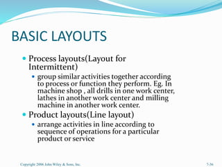
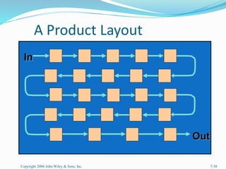
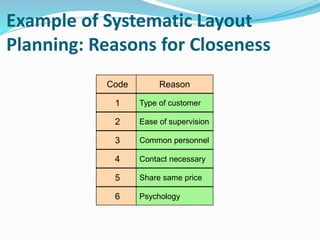
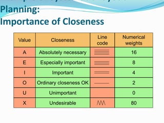
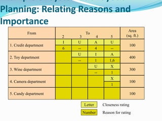
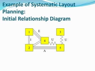
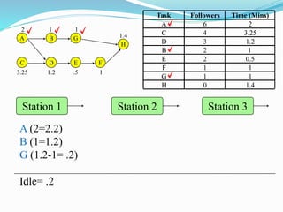
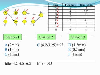
CHAPTER-6 Facility Location and Layout 1.pptx

Facility Location and Facility Layout
Kahsu Mebrahtu Areaya(Assistant Professor),
MU, CBE , MBA Program

Part I. Facility Location
 Issues in Facility Location
 Plant Location Methods

Competitive Imperatives Impacting
Location
 The need to produce close to the customer due to
time-based competition, trade agreements, and
shipping costs.
 The need to locate near the appropriate labor pool to
take advantage of low wage costs and/or high technical
skills.

Issues in Facility Location
 Proximity to Customers
 Business Climate
 Total Costs
 Infrastructure
 Quality of Labor
 Suppliers
 Other Facilities

Issues in Facility Location
 Political Risk
 Government Barriers
 Trading Blocs
 Environmental Regulation
 Competitive Advantage

The Location Decision Stages and factors
Affecting Facility Location
 Facility location decisions are commonly made in
three stages:
o The Regional Decision
o The Local Decision and
o The Site Decision

The Regional Decision
 A region may be : a country, part of a country or
province
 At this stage: economic, market and legal factors are
dominant
 The Following are specific factors of potential
importance:
o Market proximity
o Proximity to raw materials
o Availability of utilities

Cont…
o labour supply and unionization
And
Additional factors for international location decision:
o National taxes –profit taxes vs value added taxes
o Legal restrictions

The Local Decision
 This involves selecting among cities , metropolitan
areas etc.
 For example a company may decide to locate within
Zone One of Afar Region. Within this zone, the
possible local alternatives might be :Samara, Logia,
Chifra, Dubti etc.
 At this point , the following additional location factors
are relevant for consideration:

Cont…
 1. Taxes
 2. Economic incentives
free land, low-cost loans or tax abatements ,
employee training
3. Attractiveness of the community
Quality of housing, rate of crime , quality of schools,
recreational areas, etc.
4. Compatible Industry

Cont…
 5. Transportation Network
 6. Government policy and Attitude
 7. Environmental Regulations

The Site Decision
 At this stage , we need to have detail information
about the factors discussed in stage I and II
 This involves : comparing the relative availability and
costs of the needed resources such as transport ,power,
water ,land, labour, raw materials in alternative sites .

Global Location Factors
 Government stability
 Government regulations
 Political and economic systems
 Economic stability and growth
 Exchange rates
 Culture
 Climate
 Export import regulations,
duties and tariffs
 Raw material availability
 Number and proximity of
suppliers
 Transportation and
distribution system
 Labor cost and education
 Available technology
 Commercial travel
 Technical expertise
 Cross-border trade regulations
 Group trade agreements
Copyright 2006 John Wiley & Sons, Inc. Supplement 7-13

Regional Location
Factors(Summary)
 Labor (availability,
education, cost, and
unions)
 Proximity of customers
 Number of customers
 Construction/leasing
costs
 Land cost
 Modes and quality of
transportation
 Transportation costs
 Community government
Local business
regulations
 Government services
(e.g., Chamber of
Commerce)

Regional Location Factors (cont.)
 Business climate
 Community services
 Incentive packages
 Government regulations
 Environmental
regulations
 Raw material availability
 Commercial travel
 Climate
 Infrastructure (e.g., roads,
water, sewers)
 Quality of life
 Taxes
 Availability of sites
 Financial services
 Community inducements
 Proximity of suppliers
 Education system

Location Incentives
 Tax credits
 Relaxed government regulation
 Job training
 Infrastructure improvement
 Money

Location Analysis Techniques
 Location rating factor
 Center-of-gravity
 Load-distance

Location Rating Factor
 Identify important factors
 Weight factors (0.00 - 1.00)
 Subjectively score each factor (0
- 100)
 Sum weighted scores

Location Factor Rating: Example
Labor pool and climate
Proximity to suppliers
Wage rates
Community environment
Proximity to customers
Shipping modes
Air service
LOCATION FACTOR
.30
.20
.15
.15
.10
.05
.05
WEIGHT
80
100
60
75
65
85
50
Mekelle
65
91
95
80
90
92
65
Wukro
90
75
72
80
95
65
90
Addis
SCORES (0 TO 100)
Weighted Score for “Labor pool and climate” for
Mekelle =weighted value x factor score=(0.30)(80) = 24

Location Factor Rating
24.00
20.00
9.00
11.25
6.50
4.25
2.50
77.50
Mekelle
19.50
18.20
14.25
12.00
9.00
4.60
3.25
80.80
Wukro
27.00
15.00
10.80
12.00
9.50
3.25
4.50
82.05
Addis
WEIGHTED SCORES
Addis has the
highest factor rating

Center-of-Gravity
Technique
 Locate facility at center of
geographic area
 Based on weight and distance
traveled establish grid-map of
area
 Identify coordinates and
weights shipped for each
location

Plant Location Methodology: Center
of Gravity Method
 The center of gravity method is used for locating single
facilities that considers existing facilities, the distances
between them, and the volumes of goods to be shipped
between them.
 This methodology involves formulas used to compute
the coordinates of the two-dimensional point that
meets the distance and volume criteria stated above.

Plant Location Methodology: Center
of Gravity Method Formulas
C =
d V
V
x
ix i
i


Cx = X coordinate of center of gravity
Cy = Y coordinate of center of gravity
dix = X coordinate of the ith location
diy = Y coordinate of the ith location
Vi = volume of goods moved to or from ith
location
C =
d V
V
y
iy i
i



Grid-Map Coordinates
where,
x, y = coordinates of new facility
at center of gravity
xi, yi = coordinates of existing
facility i
Wi = annual weight shipped from
facility i

n
Wi
i = 1
 xiWi
i = 1
n
x =

n
Wi
i = 1
 yiWi
i = 1
n
y =
x1 x2 x3 x
y2
y
y1
y3
1 (x1, y1), W1
2 (x2, y2), W2
3 (x3, y3), W3

Center-of-Gravity Technique:
Example
A B C D
x 200 100 250 500
y 200 500 600 300
Wt 75 105 135 60
y
700
500
600
400
300
200
100
0 x
700
500 600
400
300
200
100
A
B
C
D
(135)
(105)
(75)
(60)
Miles
Miles

Center-of-Gravity Technique: Example
(cont.)
x = = = 238
n
Wi
i = 1
xiWi
i = 1
n

n
Wi
i = 1
yiWi
i = 1
n
y = = = 444
(200)(75) + (500)(105) + (600)(135) + (300)(60)
75 + 105 + 135 + 60
(200)(75) + (100)(105) + (250)(135) + (500)(60)
75 + 105 + 135 + 60

Center-of-Gravity Technique: Example
(cont.)
A B C D
x 200 100 250 500
y 200 500 600 300
Wt 75 105 135 60
y
700
500
600
400
300
200
100
0 x
700
500 600
400
300
200
100
A
B
C
D
(135)
(105)
(75)
(60)
Miles
Miles
Center of gravity (238, 444)

Load-Distance Technique
 Compute (Load x Distance) for each site
 Choose site with lowest (Load x Distance)
 Distance can be actual or straight-line

Load-Distance Calculations
 li di
i = 1
n
LD =
LD = load-distance value
li = load expressed as a weight, number of trips or units
being shipped from proposed site and location i
di = distance between proposed site and location i
di = (xi - x)2 + (yi - y)2
(x,y) = coordinates of proposed site
(xi , yi) = coordinates of existing facility
where,
where,

Load-Distance: Example
Potential Sites
Site X Y
1 360 180
2 420 450
3 250 400
Suppliers(existing facilities )
A B C D
X 200 100 250 500
Y 200 500 600 300
Wt 75 105 135 60
Compute distance from each site to each supplier
= (200-360)2 + (200-180)2
dA = (xA - x1)2 + (yA - y1)2
Site 1 = 161.2
= (100-360)2 + (500-180)2
dB = (xB - x1)2 + (yB - y1)2 = 412.3
dC = 434.2 dD = 184.4

Load-Distance: Example (cont.)
Site 2 dA = 333 dC = 226.7
dB = 323.9 dD = 170
Site 3 dA = 206.2 dC = 200
dB = 180.4 dD = 269.3
Compute load-
distance
i = 1
n
 li di
LD =
Site 1 = (75)(161.2) + (105)(412.3) + (135)(434.2) + (60)(434.4) = 125,063
Site 2 = (75)(333) + (105)(323.9) + (135)(226.7) + (60)(170) = 99,791
Site 3 = (75)(206.2) + (105)(180.3) + (135)(200) + (60)(269.3) = 77,555*
* Choose site 3

PART II: Facility Layout
ninth edition

Facility Layout
 Facility Layout and Basic Formats
 Process Layout
 Layout Planning
 Assembly Line balancing

Facility Layout
Defined
Facility layout can be defined as the process by which the
placement of departments, workgroups within departments,
workstations, machines, and stock-holding points within a
facility are determined.

Facility Layout
 Minimize material-handling
costs
 Utilize space efficiently
 Utilize labor efficiently
 Eliminate bottlenecks
 Facilitate communication and
interaction
 Reduce manufacturing cycle
time
 Reduce customer service time
 Eliminate wasted or redundant
movement
 Increase capacity
 Facilitate entry, exit, and
placement of material, products,
and people
 Incorporate safety and security
measures
 Promote product and service
quality
 Encourage proper maintenance
activities
 Provide a visual control of
activities
 Provide flexibility to adapt to
changing conditions
Copyright 2006 John Wiley & Sons, Inc. 7-35
Arrangement of areas within a facility to:

BASIC LAYOUTS
 Process layouts(Layout for
Intermittent)
 group similar activities together according
to process or function they perform. Eg. In
machine shop , all drills in one work center,
lathes in another work center and milling
machine in another work center.
 Product layouts(Line layout)
 arrange activities in line according to
sequence of operations for a particular
product or service

Manufacturing Process Layout
L
L
L
L
L
L
L
L
L
L
M
M
M
M
D
D
D
D
D
D
D
D
G
G
G
G
G
G
A A A
Receiving and
Shipping Assembly
Painting Department
Lathe Department
Milling
Department Drilling Department
Grinding
Department
P
P

A Product Layout
In
Out

Process Layout:
Systematic Layout Planning
 Numerical flow of items between departments
 Can be impractical to obtain
 Does not account for the qualitative factors that may be
crucial to the placement decision
 Systematic Layout Planning
 Accounts for the importance of having each department
located next to every other department
 Is also guided by trial and error
 Switching departments then checking the results of the
“closeness” score

Example of Systematic Layout
Planning: Reasons for Closeness
Code
1
2
3
4
5
6
Reason
Type of customer
Ease of supervision
Common personnel
Contact necessary
Share same price
Psychology

Planning:
Importance of Closeness
Value
A
E
I
O
U
X
Closeness
Line
code
Numerical
weights
Absolutely necessary
Especially important
Important
Ordinary closeness OK
Unimportant
Undesirable
16
8
4
2
0
80

Planning: Relating Reasons and
Importance
From
1. Credit department
2. Toy department
3. Wine department
4. Camera department
5. Candy department
6
I
--
U
4
A
--
U
--
U
1
I
1,6
A
--
U
1
X
1
X
To
2 3 4 5
Area
(sq. ft.)
100
400
300
100
100
Letter
Number
Closeness rating
Reason for rating

Planning:
Initial Relationship Diagram
1
2
4
3
5
U U
E
A
I

Planning:
Initial and Final Layouts
1
2 4
3
5
Initial Layout
Ignoring space and
building constraints
2
5 1 4
3
50 ft
20 ft
Final Layout
Adjusted by square
footage and building
size

Product Layout: Assembly
Balancing
 The major concern in a product layout is balancing the
assembly line so that no one workstation becomes a
bottleneck and holds up the flow of work through the
line .
 Assembly –line balancing operates under two
constraints : Precedence requirements and cycle time
restrictions

Station 1
Minutes
per Unit 6
Station 2
7
Station 3
3
Assembly Lines Balancing
Concepts
Question: Suppose you load work into the three work stations
below such that each will take the corresponding number of
minutes as shown. What is the cycle time of this line?
Answer: The cycle time of the line is always determined by
the work station taking the longest time. In this problem,
the cycle time of the line is 7 minutes. There is also going
to be idle time at the other two work stations.

Example of Line Balancing
 You’ve just been assigned the job a setting up an electric
fan assembly line with the following tasks:
Task Time (Mins) Description Predecessors
A 2 Assemble frame None
B 1 Mount switch A
C 3.25 Assemble motor housing None
D 1.2 Mount motor housing in frame A, C
E 0.5 Attach blade D
F 1 Assemble and attach safety grill E
G 1 Attach cord B
H 1.4 Test F, G

Structuring the Precedence
Diagram
Task Predecessors
A None
A
B A
B
C None
C
D A, C
D
Task Predecessors
E D
E
F E
F
G B
G
H E, G
H

Example of Line Balancing:
Precedence Diagram
Question: Which process step defines the maximum rate of
production?
A
C
B
D E F
G
H
2
3.25
1
1.2 .5
1
1.4
1
Answer: Task C is the cycle time of the line and
therefore, the maximum rate of production.

Determine Cycle Time
Question: Suppose we want to assemble 100 fans
per day. What would our cycle time have to be?
Required Cycle Time, C =
Production time per period
Required output per period
C =
420 mins / day
100 units / day
= 4.2 mins / unit
Answer:

Example of Line Balancing: Determine Theoretical
Minimum Number of Workstations
Question: What is the theoretical minimum number of
workstations for this problem?
Answer: Theoretical Min. Number of Workstations, N
N =
Sum of task times (T)
Cycle time (C)
t
t
N =
11.35 mins / unit
4.2 mins / unit
= 2.702, or 3
t

To Follow for Loading
Workstations
 1. Draw the precedence diagram for all tasks
 2.Group the elemental tasks without exceeding the cycle time.
 3.Calculate the efficiency of the line

A
C
B
D E F
G
H
2
3.25
1
1.2 .5
1
1.4
1
Station 1 Station 2 Station 3
Task Followers Time (Mins)
A 6 2
C 4 3.25
D 3 1.2
B 2 1
E 2 0.5
F 1 1
G 1 1
H 0 1.4

A
C
B
D E F
G
H
2
3.25
1
1.2 .5
1
1.4
1
A (2min)
A 6 2
C 4 3.25
D 3 1.2
B 2 1
E 2 0.5
F 1 1
G 1 1
H 0 1.4

A
C
B
D E F
G
H
2
3.25
1
1.2 .5
1
1.4
1
A (4.2-2=2.2)
B (2.2-1=1.2)
A 6 2
C 4 3.25
D 3 1.2
B 2 1
E 2 0.5
F 1 1
G 1 1
H 0 1.4

A
C
B
D E F
G
H
2
3.25
1
1.2 .5
1
1.4
1
A (2=2.2)
B (1=1.2)
G (1.2-1= .2)
Idle= .2
A 6 2
C 4 3.25
D 3 1.2
B 2 1
E 2 0.5
F 1 1
G 1 1
H 0 1.4

A
C
B
D E F
G
H
2
3.25
1
1.2 .5
1
1.4
1
C (4.2-3.25)=.95
A 6 2
C 4 3.25
D 3 1.2
B 2 1
E 2 0.5
F 1 1
G 1 1
H 0 1.4
A (4.2-2=2.2)
B (2.2-1=1.2)
G (1.2-1= .2)
Idle= .2

C (4.2-3.25)=.95
Idle = .95
A
C
B
D E F
G
H
2
3.25
1
1.2 .5
1
1.4
1
A 6 2
C 4 3.25
D 3 1.2
B 2 1
E 2 0.5
F 1 1
G 1 1
H 0 1.4
A (2)
B (1)
G (1)
Idle=4.2-4= .2

C (3.25)
Idle =4.2-3.25= .95
A
C
B
D E F
G
H
2
3.25
1
1.2 .5
1
1.4
1
D (1.2)
A 6 2
C 4 3.25
D 3 1.2
B 2 1
E 2 0.5
F 1 1
G 1 1
H 0 1.4
A (2)
B (1)
G (1)
Idle=4.2-4= .2

A
C
B
D E F
G
H
2
3.25
1
1.2 .5
1
1.4
1
C (3.25)
Idle =4.2-3.25= .95
D (1.2)
E (.5)
A 6 2
C 4 3.25
D 3 1.2
B 2 1
E 2 0.5
F 1 1
G 1 1
H 0 1.4
A(2min)
B (1min)
G (1min
Idle=4.2-4=.2

A
C
B
D E F
G
H
2
3.25
1
1.2 .5
1
1.4
1
C (4.2-3.25)=.95
Idle = .95
D (1.2min)
E (0.5min)
F (1min)
A 6 2
C 4 3.25
D 3 1.2
B 2 1
E 2 0.5
F 1 1
G 1 1
H 0 1.4
A (2min)
B (1min)
G (1min)
Idle=4.2-4.0=0.2

Which station is the bottleneck? What is the effective cycle time?
A
C
B
D E F
G
H
2
3.25
1
1.2 .5
1
1.4
1
C (3.25)
Idle4.2-3.25 = .95
D (1.2min)
E (.5min)
F (1min)
H (1.4min)
Idle 4.2-4.1= .1
A 6 2
C 4 3.25
D 3 1.2
B 2 1
E 2 0.5
F 1 1
G 1 1
H 0 1.4
A (2min)
B (1min)
G (1min)
Idle=4.2-4= .2

Determine the Efficiency of the
Assembly Line
33.78%
=
s/unit)
(8)(4.2min
mins/unit
11.35
=
Efficiency
Efficiency =
Sum of task times (T)
Actual number of workstations (Na) x Cycle time (C)

Cont…
0.1%
9
=
s/unit)
(3)(4.2min
mins/unit
11.35
=
Efficiency

Cont…
 Balanced delay=100-Efficiency
=100-90.1
=9.9%

Reading Assignment
1.Group Technology
2. Fixed position layout
3.Service operations layout

 Exercise
An assembly line with 17 tasks is to be balanced . The longest task is 2.4
minutes , and the total time for all tasks is 18 minutes. The line will
operate for 450 minutes per day.
a. what are the minimum and maximum cycle time?
b. What range of output is theoretically possible for the line ?
c. What is the minimum number of workstations needed if the maximum
output rate is to be sought ?
d. What cycle time will provide an output rate of 125 units per day?
e. What output potential will result if the cycle time is (1) 9 minutes ? (2)
15 minutes ?

CHAPTER-6 Facility Location and Layout 1.pptx

More Related Content

What's hot

Similar to CHAPTER-6 Facility Location and Layout 1.pptx

More from amanuel236786

Recently uploaded

CHAPTER-6 Facility Location and Layout 1.pptx

Editor's Notes