Chapter 3

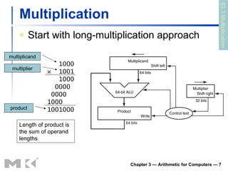
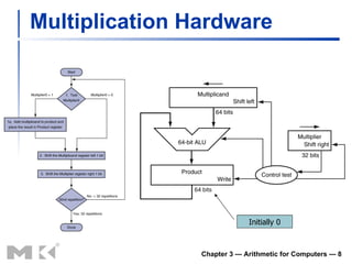
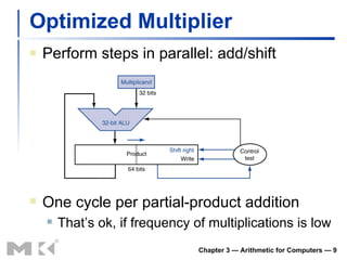
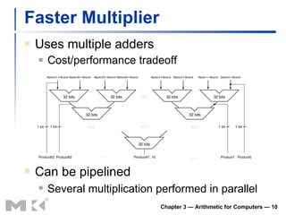
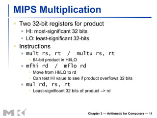
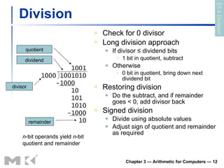
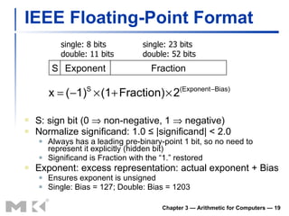
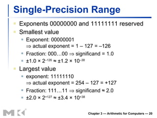
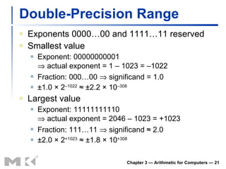
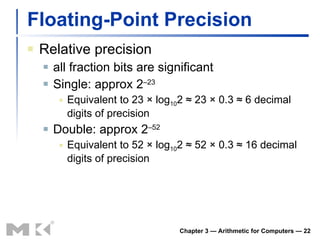
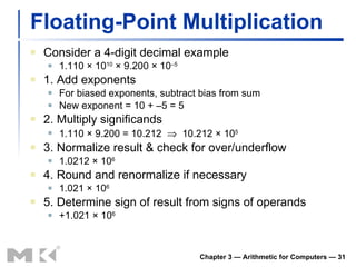
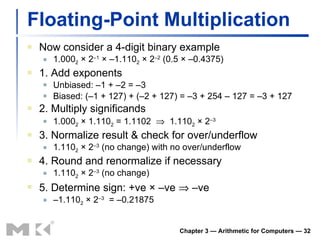
Chapter 3 Arithmetic for Computers

Arithmetic for Computers Operations on integers Addition and subtraction Multiplication and division Dealing with overflow Floating-point real numbers Representation and operations Chapter 3 — Arithmetic for Computers — §3.1 Introduction

Integer Addition Example: 7 + 6 Chapter 3 — Arithmetic for Computers — §3.2 Addition and Subtraction Overflow if result out of range Adding +ve and –ve operands, no overflow Adding two +ve operands Overflow if result sign is 1 Adding two –ve operands Overflow if result sign is 0

Integer Subtraction Add negation of second operand Example: 7 – 6 = 7 + (–6) +7: 0000 0000 … 0000 0111 –6: 1111 1111 … 1111 1010 +1: 0000 0000 … 0000 0001 Overflow if result out of range Subtracting two +ve or two –ve operands, no overflow Subtracting +ve from –ve operand Overflow if result sign is 0 Subtracting –ve from +ve operand Overflow if result sign is 1 Chapter 3 — Arithmetic for Computers —

Dealing with Overflow Some languages (e.g., C) ignore overflow Use MIPS addu , addui , subu instructions Other languages (e.g., Ada, Fortran) require raising an exception Use MIPS add , addi , sub instructions On overflow, invoke exception handler Save PC in exception program counter (EPC) register Jump to predefined handler address mfc0 (move from coprocessor reg) instruction can retrieve EPC value, to return after corrective action Chapter 3 — Arithmetic for Computers —

Arithmetic for Multimedia Graphics and media processing operates on vectors of 8-bit and 16-bit data Use 64-bit adder, with partitioned carry chain Operate on 8 ×8-bit, 4×16-bit, or 2×32-bit vectors SIMD (single-instruction, multiple-data) Saturating operations On overflow, result is largest representable value c.f. 2s-complement modulo arithmetic E.g., clipping in audio, saturation in video Chapter 3 — Arithmetic for Computers —

Multiplication Start with long-multiplication approach Chapter 3 — Arithmetic for Computers — Length of product is the sum of operand lengths multiplicand multiplier product §3.3 Multiplication 1000 × 1001 1000 0000 0000 1000 1001000

Multiplication Hardware Chapter 3 — Arithmetic for Computers — Initially 0

Optimized Multiplier Perform steps in parallel: add/shift Chapter 3 — Arithmetic for Computers — One cycle per partial-product addition That’s ok, if frequency of multiplications is low

Faster Multiplier Uses multiple adders Cost/performance tradeoff Chapter 3 — Arithmetic for Computers — Can be pipelined Several multiplication performed in parallel

MIPS Multiplication Two 32-bit registers for product HI: most-significant 32 bits LO: least-significant 32-bits Instructions mult rs, rt / multu rs, rt 64-bit product in HI/LO mfhi rd / mflo rd Move from HI/LO to rd Can test HI value to see if product overflows 32 bits mul rd, rs, rt Least-significant 32 bits of product –> rd Chapter 3 — Arithmetic for Computers —

Division Check for 0 divisor Long division approach If divisor ≤ dividend bits 1 bit in quotient, subtract Otherwise 0 bit in quotient, bring down next dividend bit Restoring division Do the subtract, and if remainder goes < 0, add divisor back Signed division Divide using absolute values Adjust sign of quotient and remainder as required Chapter 3 — Arithmetic for Computers — 1001 1000 1001010 -1000 10 101 1010 -1000 10 n -bit operands yield n -bit quotient and remainder quotient dividend remainder divisor §3.4 Division

Division Hardware Chapter 3 — Arithmetic for Computers — Initially dividend Initially divisor in left half

Optimized Divider One cycle per partial-remainder subtraction Looks a lot like a multiplier! Same hardware can be used for both Chapter 3 — Arithmetic for Computers —

Faster Division Can’t use parallel hardware as in multiplier Subtraction is conditional on sign of remainder Faster dividers (e.g. SRT devision) generate multiple quotient bits per step Still require multiple steps Chapter 3 — Arithmetic for Computers —

MIPS Division Use HI/LO registers for result HI: 32-bit remainder LO: 32-bit quotient Instructions div rs, rt / divu rs, rt No overflow or divide-by-0 checking Software must perform checks if required Use mfhi , mflo to access result Chapter 3 — Arithmetic for Computers —

Floating Point Representation for non-integral numbers Including very small and very large numbers Like scientific notation – 2.34 × 10 56 +0.002 × 10 –4 +987.02 × 10 9 In binary ±1. xxxxxxx 2 × 2 yyyy Types float and double in C Chapter 3 — Arithmetic for Computers — normalized not normalized §3.5 Floating Point

Floating Point Standard Defined by IEEE Std 754-1985 Developed in response to divergence of representations Portability issues for scientific code Now almost universally adopted Two representations Single precision (32-bit) Double precision (64-bit) Chapter 3 — Arithmetic for Computers —

IEEE Floating-Point Format S: sign bit (0  non-negative, 1  negative) Normalize significand: 1.0 ≤ |significand| < 2.0 Always has a leading pre-binary-point 1 bit, so no need to represent it explicitly (hidden bit) Significand is Fraction with the “1.” restored Exponent: excess representation: actual exponent + Bias Ensures exponent is unsigned Single: Bias = 127; Double: Bias = 1203 Chapter 3 — Arithmetic for Computers — S Exponent Fraction single: 8 bits double: 11 bits single: 23 bits double: 52 bits

Single-Precision Range Exponents 00000000 and 11111111 reserved Smallest value Exponent: 00000001  actual exponent = 1 – 127 = –126 Fraction: 000…00  significand = 1.0 ±1.0 × 2 –126 ≈ ±1.2 × 10 –38 Largest value exponent: 11111110  actual exponent = 254 – 127 = +127 Fraction: 111…11  significand ≈ 2.0 ±2.0 × 2 +127 ≈ ±3.4 × 10 +38 Chapter 3 — Arithmetic for Computers —

Double-Precision Range Exponents 0000…00 and 1111…11 reserved Smallest value Exponent: 00000000001  actual exponent = 1 – 1023 = –1022 Fraction: 000…00  significand = 1.0 ±1.0 × 2 –1022 ≈ ±2.2 × 10 –308 Largest value Exponent: 11111111110  actual exponent = 2046 – 1023 = +1023 Fraction: 111…11  significand ≈ 2.0 ±2.0 × 2 +1023 ≈ ±1.8 × 10 +308 Chapter 3 — Arithmetic for Computers —

Floating-Point Precision Relative precision all fraction bits are significant Single: approx 2 –23 Equivalent to 23 × log 10 2 ≈ 23 × 0.3 ≈ 6 decimal digits of precision Double: approx 2 –52 Equivalent to 52 × log 10 2 ≈ 52 × 0.3 ≈ 16 decimal digits of precision Chapter 3 — Arithmetic for Computers —

Floating-Point Example Represent –0.75 – 0.75 = (–1) 1 × 1.1 2 × 2 –1 S = 1 Fraction = 1000…00 2 Exponent = –1 + Bias Single: –1 + 127 = 126 = 01111110 2 Double: –1 + 1023 = 1022 = 01111111110 2 Single: 1 01111110 1000…00 Double: 1 01111111110 1000…00 Chapter 3 — Arithmetic for Computers —

Floating-Point Example What number is represented by the single-precision float 1 10000001 01000…00 S = 1 Fraction = 01000…00 2 Fxponent = 10000001 2 = 129 x = (–1) 1 × (1 + 01 2 ) × 2 (129 – 127) = (–1) × 1.25 × 2 2 = –5.0 Chapter 3 — Arithmetic for Computers —

Denormal Numbers Exponent = 000...0  hidden bit is 0 Chapter 3 — Arithmetic for Computers — Smaller than normal numbers allow for gradual underflow, with diminishing precision Denormal with fraction = 000...0 Two representations of 0.0!

Infinities and NaNs Exponent = 111...1, Fraction = 000...0 ±Infinity Can be used in subsequent calculations, avoiding need for overflow check Exponent = 111...1, Fraction ≠ 000...0 Not-a-Number (NaN) Indicates illegal or undefined result e.g., 0.0 / 0.0 Can be used in subsequent calculations Chapter 3 — Arithmetic for Computers —

Floating-Point Addition Consider a 4-digit decimal example 9.999 × 10 1 + 1.610 × 10 –1 1. Align decimal points Shift number with smaller exponent 9.999 × 10 1 + 0.016 × 10 1 2. Add significands 9.999 × 10 1 + 0.016 × 10 1 = 10.015 × 10 1 3. Normalize result & check for over/underflow 1.0015 × 10 2 4. Round and renormalize if necessary 1.002 × 10 2 Chapter 3 — Arithmetic for Computers —

Floating-Point Addition Now consider a 4-digit binary example 1.000 2 × 2 –1 + –1.110 2 × 2 –2 (0.5 + –0.4375) 1. Align binary points Shift number with smaller exponent 1.000 2 × 2 –1 + –0.111 2 × 2 –1 2. Add significands 1.000 2 × 2 –1 + –0.111 2 × 2 – 1 = 0.001 2 × 2 –1 3. Normalize result & check for over/underflow 1.000 2 × 2 –4 , with no over/underflow 4. Round and renormalize if necessary 1.000 2 × 2 –4 (no change) = 0.0625 Chapter 3 — Arithmetic for Computers —

FP Adder Hardware Much more complex than integer adder Doing it in one clock cycle would take too long Much longer than integer operations Slower clock would penalize all instructions FP adder usually takes several cycles Can be pipelined Chapter 3 — Arithmetic for Computers —

FP Adder Hardware Chapter 3 — Arithmetic for Computers — Step 1 Step 2 Step 3 Step 4

Floating-Point Multiplication Consider a 4-digit decimal example 1.110 × 10 10 × 9.200 × 10 –5 1. Add exponents For biased exponents, subtract bias from sum New exponent = 10 + –5 = 5 2. Multiply significands 1.110 × 9.200 = 10.212  10.212 × 10 5 3. Normalize result & check for over/underflow 1.0212 × 10 6 4. Round and renormalize if necessary 1.021 × 10 6 5. Determine sign of result from signs of operands +1.021 × 10 6 Chapter 3 — Arithmetic for Computers —

Floating-Point Multiplication Now consider a 4-digit binary example 1.000 2 × 2 –1 × –1.110 2 × 2 –2 (0.5 × –0.4375) 1. Add exponents Unbiased: –1 + –2 = –3 Biased: (–1 + 127) + (–2 + 127) = –3 + 254 – 127 = –3 + 127 2. Multiply significands 1.000 2 × 1.110 2 = 1.1102  1.110 2 × 2 –3 3. Normalize result & check for over/underflow 1.110 2 × 2 –3 (no change) with no over/underflow 4. Round and renormalize if necessary 1.110 2 × 2 –3 (no change) 5. Determine sign: +ve × –ve  –ve – 1.110 2 × 2 –3 = –0.21875 Chapter 3 — Arithmetic for Computers —

FP Arithmetic Hardware FP multiplier is of similar complexity to FP adder But uses a multiplier for significands instead of an adder FP arithmetic hardware usually does Addition, subtraction, multiplication, division, reciprocal, square-root FP  integer conversion Operations usually takes several cycles Can be pipelined Chapter 3 — Arithmetic for Computers —

FP Instructions in MIPS FP hardware is coprocessor 1 Adjunct processor that extends the ISA Separate FP registers 32 single-precision: $f0, $f1, … $f31 Paired for double-precision: $f0/$f1, $f2/$f3, … Release 2 of MIPs ISA supports 32 × 64-bit FP reg’s FP instructions operate only on FP registers Programs generally don’t do integer ops on FP data, or vice versa More registers with minimal code-size impact FP load and store instructions lwc1 , ldc1 , swc1 , sdc1 e.g., ldc1 $f8, 32($sp) Chapter 3 — Arithmetic for Computers —

FP Instructions in MIPS Single-precision arithmetic add.s , sub.s , mul.s , div.s e.g., add.s $f0, $f1, $f6 Double-precision arithmetic add.d , sub.d , mul.d , div.d e.g., mul.d $f4, $f4, $f6 Single- and double-precision comparison c. xx .s , c. xx .d ( xx is eq , lt , le , …) Sets or clears FP condition-code bit e.g. c.lt.s $f3, $f4 Branch on FP condition code true or false bc1t , bc1f e.g., bc1t TargetLabel Chapter 3 — Arithmetic for Computers —

FP Example: °F to °C C code: float f2c (float fahr) { return ((5.0/9.0)*(fahr - 32.0)); } fahr in $f12, result in $f0, literals in global memory space Compiled MIPS code: f2c: lwc1 $f16, const5($gp) lwc2 $f18, const9($gp) div.s $f16, $f16, $f18 lwc1 $f18, const32($gp) sub.s $f18, $f12, $f18 mul.s $f0, $f16, $f18 jr $ra Chapter 3 — Arithmetic for Computers —

FP Example: Array Multiplication X = X + Y × Z All 32 × 32 matrices, 64-bit double-precision elements C code: void mm (double x[][], double y[][], double z[][]) { int i, j, k; for (i = 0; i! = 32; i = i + 1) for (j = 0; j! = 32; j = j + 1) for (k = 0; k! = 32; k = k + 1) x[i][j] = x[i][j] + y[i][k] * z[k][j]; } Addresses of x , y , z in $a0, $a1, $a2, and i , j , k in $s0, $s1, $s2 Chapter 3 — Arithmetic for Computers —

FP Example: Array Multiplication Chapter 3 — Arithmetic for Computers — MIPS code: li $t1, 32 # $t1 = 32 (row size/loop end) li $s0, 0 # i = 0; initialize 1st for loop L1: li $s1, 0 # j = 0; restart 2nd for loop L2: li $s2, 0 # k = 0; restart 3rd for loop sll $t2, $s0, 5 # $t2 = i * 32 (size of row of x) addu $t2, $t2, $s1 # $t2 = i * size(row) + j sll $t2, $t2, 3 # $t2 = byte offset of [i][j] addu $t2, $a0, $t2 # $t2 = byte address of x[i][j] l.d $f4, 0($t2) # $f4 = 8 bytes of x[i][j] L3: sll $t0, $s2, 5 # $t0 = k * 32 (size of row of z) addu $t0, $t0, $s1 # $t0 = k * size(row) + j sll $t0, $t0, 3 # $t0 = byte offset of [k][j] addu $t0, $a2, $t0 # $t0 = byte address of z[k][j] l.d $f16, 0($t0) # $f16 = 8 bytes of z[k][j] …

FP Example: Array Multiplication Chapter 3 — Arithmetic for Computers — … sll $t0, $s0, 5 # $t0 = i*32 (size of row of y) addu $t0, $t0, $s2 # $t0 = i*size(row) + k sll $t0, $t0, 3 # $t0 = byte offset of [i][k] addu $t0, $a1, $t0 # $t0 = byte address of y[i][k] l.d $f18, 0($t0) # $f18 = 8 bytes of y[i][k] mul.d $f16, $f18, $f16 # $f16 = y[i][k] * z[k][j] add.d $f4, $f4, $f16 # f4=x[i][j] + y[i][k]*z[k][j] addiu $s2, $s2, 1 # $k k + 1 bne $s2, $t1, L3 # if (k != 32) go to L3 s.d $f4, 0($t2) # x[i][j] = $f4 addiu $s1, $s1, 1 # $j = j + 1 bne $s1, $t1, L2 # if (j != 32) go to L2 addiu $s0, $s0, 1 # $i = i + 1 bne $s0, $t1, L1 # if (i != 32) go to L1

Accurate Arithmetic IEEE Std 754 specifies additional rounding control Extra bits of precision (guard, round, sticky) Choice of rounding modes Allows programmer to fine-tune numerical behavior of a computation Not all FP units implement all options Most programming languages and FP libraries just use defaults Trade-off between hardware complexity, performance, and market requirements Chapter 3 — Arithmetic for Computers —

Interpretation of Data Bits have no inherent meaning Interpretation depends on the instructions applied Computer representations of numbers Finite range and precision Need to account for this in programs Chapter 3 — Arithmetic for Computers — The BIG Picture

Associativity Parallel programs may interleave operations in unexpected orders Assumptions of associativity may fail Chapter 3 — Arithmetic for Computers — §3.6 Parallelism and Computer Arithmetic: Associativity Need to validate parallel programs under varying degrees of parallelism

x86 FP Architecture Originally based on 8087 FP coprocessor 8 × 80-bit extended-precision registers Used as a push-down stack Registers indexed from TOS: ST(0), ST(1), … FP values are 32-bit or 64 in memory Converted on load/store of memory operand Integer operands can also be converted on load/store Very difficult to generate and optimize code Result: poor FP performance Chapter 3 — Arithmetic for Computers — §3.7 Real Stuff: Floating Point in the x86

x86 FP Instructions Optional variations I : integer operand P : pop operand from stack R : reverse operand order But not all combinations allowed Chapter 3 — Arithmetic for Computers — Data transfer Arithmetic Compare Transcendental F I LD mem/ST(i) F I ST P mem/ST(i) FLDPI FLD1 FLDZ F I ADD P mem/ST(i) F I SUB RP mem/ST(i) F I MUL P mem/ST(i) F I DIV RP mem/ST(i) FSQRT FABS FRNDINT F I COM P F I UCOM P FSTSW AX/mem FPATAN F2XMI FCOS FPTAN FPREM FPSIN FYL2X

Streaming SIMD Extension 2 (SSE2) Adds 4 × 128-bit registers Extended to 8 registers in AMD64/EM64T Can be used for multiple FP operands 2 × 64-bit double precision 4 × 32-bit double precision Instructions operate on them simultaneously S ingle- I nstruction M ultiple- D ata Chapter 3 — Arithmetic for Computers —

Right Shift and Division Left shift by i places multiplies an integer by 2 i Right shift divides by 2 i ? Only for unsigned integers For signed integers Arithmetic right shift: replicate the sign bit e.g., –5 / 4 1 1111011 2 >> 2 = 111 11110 2 = –2 Rounds toward –∞ c.f. 1 1111011 2 >>> 2 = 001 11110 2 = +62 Chapter 3 — Arithmetic for Computers — §3.8 Fallacies and Pitfalls

Who Cares About FP Accuracy? Important for scientific code But for everyday consumer use? “ My bank balance is out by 0.0002¢!”  The Intel Pentium FDIV bug The market expects accuracy See Colwell, The Pentium Chronicles Chapter 3 — Arithmetic for Computers —

Concluding Remarks ISAs support arithmetic Signed and unsigned integers Floating-point approximation to reals Bounded range and precision Operations can overflow and underflow MIPS ISA Core instructions: 54 most frequently used 100% of SPECINT, 97% of SPECFP Other instructions: less frequent Chapter 3 — Arithmetic for Computers — §3.9 Concluding Remarks

Chapter 3

More Related Content

What's hot

Similar to Chapter 3

More from ececourse

Chapter 3

Editor's Notes