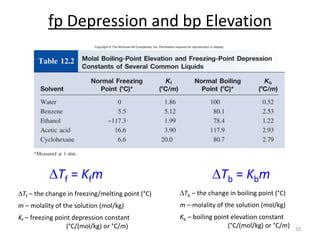
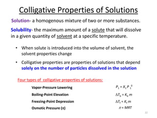
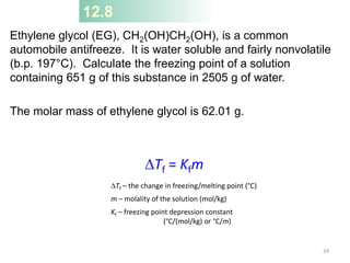
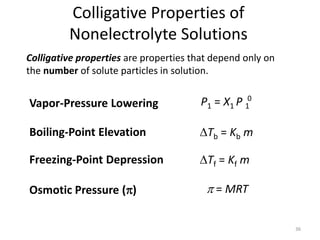
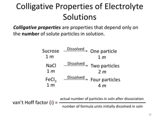
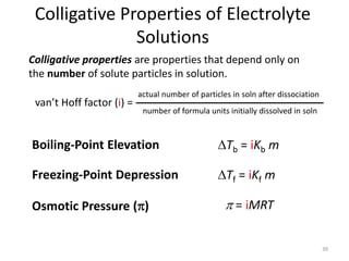
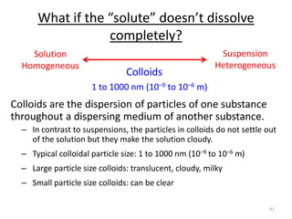
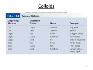
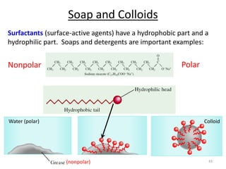
Chapter 12
Ch 12
Page 520 1
Colligative Properties of Solutions
• When solute is introduced into the volume of solvent, the
solvent properties change
• Colligative properties are properties of solutions that depend
solely on the number of particles dissolved in the solution
2
Vapor-Pressure Lowering P1 = X1 P 1
0
Boiling-Point Elevation DTb = Kb m
Freezing-Point Depression DTf = Kf m
Osmotic Pressure (p) p = MRT
Solution- a homogenous mixture of two or more substances.
Solubility- the maximum amount of a solute that will dissolve
in a given quantity of solvent at a specific temperature.
Four types of colligative properties of solutions:
strong
driving
force
Vapor-Pressure Lowering
Occurs with non-volatile, non-ionizing solutes at low solute concentrations.
~0 vapor pressure does not dissociate
Solute molecule
The vapor pressure of a pure solvent drops
whenever non-volatile solute is added.
“Ordered”
disordered
Liquid
Gas
less
“Ordered”
disordered
weaker
driving
force
Larger
entropy
increase
Smaller
entropy
increase
3
Raoult’s Law (Vapor Pressure Lowering)
• The vapor pressure (P1 ) of a solvent is directly proportional to
the mole fraction (X1 ) of the solvent in the solution
• Raoult’s Law:
P1 = X1  P0
1
(P 0
1 – vapor pressure of the pure solvent)
4
vapor pressure (P1) ∝ mole fraction of solvent(X1)
As solute is added, the vapor pressure drops.
X1 P1
For pure solvent X1 = 1.0,
and
X1 =
moles of solvent
moles of solvent + moles of solute
P1 = P0
1
moles of solute
• P 0
1 – the vapor pressure of the pure solvent
P1 – the vapor pressure of the solution with solute
5
Raoult’s Law (Vapor Pressure Lowering)
X1 =
moles of solvent
moles of solvent + moles of solute
P1 = (1–X2)  P0
1
X2 =
moles of solute
moles of solvent + moles of solute
X1 = (1 – X2)
P1 = P0
1 – X2 P0
1
P0
1 – P1 = X2 P0
1
DP = X2 P0
1
P1 = X1  P0
1
12.7
Calculate the vapor pressure of a solution made by dissolving
218 g of glucose (molar mass = 180.2 g/mol) in 460 mL of water
at 30°C (PH2O = 31.82 mmHg). Assume the density of the
solvent is 1.00 g/mL.
What is the vapor-pressure lowering?
P1 = X1  P0
1
P0
1 = vapor pressure of pure solvent
P1 = vapor pressure of the solution
X1 = mole fraction of solvent
6
12.7
Solution The vapor pressure of a solution (P1) is
First we calculate the number of moles of glucose and water in
the solution:
The mole fraction of water, X1, is given by
7
12.7
The vapor pressure of water at 30°C is31.82 mmHg. Therefore,
the vapor pressure of the glucose solution is
Finally, the vapor-pressure lowering (DP) is
(31.82 − 30.4) mmHg, or 1.4 mmHg.
Or you could use:
P1 = 0.955  31.82 mmHg
= 30.4 mmHg
DP = X2 P0
1
8
Vapor-Pressure Lowering
Talked about with non-volatile, non-ionizing solutes.
The vapor pressure = the sum of the vapor pressure of the components.
The vapor pressure for the solvent is reduced.
What about volatile solutes (solutes with a vapor pressure).
Example: Ethanol in water.
Liquid
Gas
Solute molecule
9
Raoult’s Law (Liquid-Liquid Mixture)
• If components A and B of a solution are volatile,
Raoult’s law still holds:
PA = XAP0
A
PB = XBP0
B
PT = PA + PB
PT = XAP0
A + XBP0
B
• Assuming it is an ideal solution
• For an ideal solution, DHsoln = 0
10
DHsoln = DH1 + DH2 + DH3
A
B
Ideal if:
solvent-solute interaction = solute-solute + solvent-solvent
11
Raoult’s Law (Liquid-Liquid Mixture)
Benzene and toluene form an “ideal” solution
PA = XAP0
A
PB = XBP0
B
PT = PA + PB
PT = XAP0
A + XBP0
B
benzene
(A)
toluene
(B)
Benzene and toluene similar structures, similar forces (dispersion forces).
What about other liquid-liquid mixtures?
12
Force
A-B
Force
A-A
Force
B-B
< +
Most solutions are nonideal and deviate from Raoult’s law!
Positive Deviation Negative Deviation
PA, PB and PT are greater than predicted
A and B hate each other
and want to get out!
Raoult’s Law (Liquid-Liquid Mixture)
PA, PB and PT are smaller than predicted
Force
A-B
Force
A-A
Force
B-B
> +
A and B like each other
and want to stay together!
Solutions and Cooking
13
Adding salt (non-volatile solute) to water (solvent) will:
1) reduce the time it takes to heat up.
2) make the water boil hotter.
Solutions and Cooking
Raoult’s law:
14
Adding salt (non-volatile solute) to water (solvent)
As solute is added, the vapor pressure decreases, more energy
(higher boiling point) is required for the vapor pressure to equal
atmospheric pressure!
X1 P1
moles of solute
P1 = X1  P0
1
P0
1 = vapor pressure of pure solvent
P1 = vapor pressure of the solution
X1 = mole fraction of solvent
Boiling Pt
AKA Boiling Point Elevation.
Boiling Point Elevation
• As expected from Raoult’s law, which predicts lower vapor
pressure, boiling temperature elevation is determined by the
number of moles of solute dissolved in the solution:
• DTb – the change in boiling point (°C)
• m – molality of the solution (mol/kg)
• Kb – boiling point elevation constant (°C/(mol/kg) or °C/m)
15
DTb = Kbm
change in bp temperature (DTb) ∝ molality of the solution (m)
Note: the Kb value only depends on the solvent
the molality, m depends on the concentration of solute
Solutions and Cooking
16
Adding salt (non-volatile solute) to water (solvent) will:
1) make the water boil hotter
2) reduce the time it takes to heat up.
The boiling point of water increases from 100°C (212°F)
to 102°C (216°F) upon the addition of salt.
Freezing Point Depression
17
Freezing Point Depression
• Addition of a nonvolatile solute to a solution lowers the freezing
point of the solution relative to the pure solvent:
• DTf – the change in freezing/melting point (°C)
• m – molality of the solution (mol/kg)
• Kf – freezing point depression constant (°C/(mol/kg) or °C/m)
18
DTf = Kfm
change in freezing temperature (DTb) ∝ molality of the solution
(m)
Note: the Kf value only depends on the solvent
the molality, m depends on the concentration of solute
Phase Diagram Solution vs Water
Boiling
point
elevation
Freezing
point
depression
19
20
DTf = Kfm
DTf – the change in freezing/melting point (°C)
m – molality of the solution (mol/kg)
Kf – freezing point depression constant
(°C/(mol/kg) or °C/m)
DTb = Kbm
DTb – the change in boiling point (°C)
m – molality of the solution (mol/kg)
Kb – boiling point elevation constant
(°C/(mol/kg) or °C/m)
fp Depression and bp Elevation
Chapter 12
21
Colligative Properties of Solutions
• When solute is introduced into the volume of solvent, the
solvent properties change
• Colligative properties are properties of solutions that depend
solely on the number of particles dissolved in the solution
22
Vapor-Pressure Lowering P1 = X1 P 1
0
Boiling-Point Elevation DTb = Kb m
Freezing-Point Depression DTf = Kf m
Osmotic Pressure (p) p = MRT
Solution- a homogenous mixture of two or more substances.
Solubility- the maximum amount of a solute that will dissolve
in a given quantity of solvent at a specific temperature.
Four types of colligative properties of solutions:
23
DTf = Kfm
DTf – the change in freezing/melting point (°C)
m – molality of the solution (mol/kg)
Kf – freezing point depression constant
(°C/(mol/kg) or °C/m)
DTb = Kbm
DTb – the change in boiling point (°C)
m – molality of the solution (mol/kg)
Kb – boiling point elevation constant
(°C/(mol/kg) or °C/m)
fp Depression and bp Elevation
12.8
Ethylene glycol (EG), CH2(OH)CH2(OH), is a common
automobile antifreeze. It is water soluble and fairly nonvolatile
(b.p. 197°C). Calculate the freezing point of a solution
containing 651 g of this substance in 2505 g of water.
The molar mass of ethylene glycol is 62.01 g.
DTf = Kfm
DTf – the change in freezing/melting point (°C)
m – molality of the solution (mol/kg)
Kf – freezing point depression constant
(°C/(mol/kg) or °C/m)
24
12.8
Strategy
Solution To solve for the molality of the solution, we need to
know the number of moles of EG and the mass of the solvent in
kilograms.
25
We fi nd the molar mass of EG, and convert the mass of the
solvent to 2.505 kg, and calculate the molality as follows:
From the table, Kf = 1.86 °C/m. Therefore:
12.8
Because pure water freezes at 0°C, the solution will freeze at
(0 − 7.79)°C. 26
27
3% salt
solution
selectively
permeable
membrane
distilled
water
salt
solution
rising
solution stops rising when
weight of column equals
osmotic pressure
Osmosis
Osmosis is the selective passage of solvent molecules through a porous membrane
from a dilute solution to a more concentrated one.
A semipermeable membrane allows the passage of solvent molecules but blocks the
passage of solute molecules.
28
High P
Low P
solvent solution
time
More out
than in
less out
than in
Alternative View
A semipermeable membrane
allows the passage of solvent
molecules but blocks the
passage of solute molecules.
29
Osmosis is the selective passage of solvent molecules through a porous membrane
from a dilute solution to a more concentrated one.
A semipermeable membrane allows the passage of solvent molecules but blocks the
passage of solute molecules.
Osmosis
Pure
Solvent Solution
“Higher
vapor
pressure”
“Lower
vapor
pressure”
Osmotic pressure (p) is the pressure required to stop osmosis.
30
Osmotic Pressure
• Osmosis is a rate controlled phenomenon.
– The solvent is passing from the dilute solution into
the concentrated solution at a faster rate than in
opposite direction, i.e. establishing an equilibrium.
• The osmotic pressure
MRT

p
(K)
re
temperatu
absolute
=
K
mol
atm
L
0.0821
=
(mol/L)
solution
of
ion
concentrat
molar
=
(atm)
pressure
osmotic
=
T
R
M
p
12.9
The average osmotic pressure of seawater, measured in the
kind of apparatus shown below, is about 30.0 atm at 25°C.
Calculate the molar concentration of an aqueous solution of
sucrose (C12H22O11) that is isotonic with seawater.
MRT

p
31
12.9
Strategy When we say the sucrose solution is isotonic with
seawater, what can we conclude about the osmotic pressures
of these two solutions?
Solution A solution of sucrose that is isotonic with seawater
must have the same osmotic pressure, 30.0 atm. Using
Equation (12.8).
32
12.11
A solution is prepared by dissolving 35.0 g of hemoglobin (Hb)
in enough water to make up 1 L in volume. If the osmotic
pressure of the solution is found to be 10.0 mmHg at 25°C,
calculate the molar mass of hemoglobin.
MRT

p
We have p, R and T
Find M
33
12.11
First we calculate the molarity:
The volume of the solution is 1 L, so it must contain
5.38 × 10⁻⁴ mol of Hb.
We use this quantity to calculate the molar mass:
34
Reverse Osmosis
• Used world-wide to purify sea water.
• Ft. Myers, FL gets it drinking water from the Gulf of
Mexico using reverse osmosis.
• US Navy submarines do as well.
• Dialysis is another example of this phenomenon.
35
36
Colligative Properties of
Nonelectrolyte Solutions
Vapor-Pressure Lowering P1 = X1 P 1
0
Boiling-Point Elevation DTb = Kb m
Freezing-Point Depression DTf = Kf m
Osmotic Pressure (p) p = MRT
Colligative properties are properties that depend only on
the number of solute particles in solution.
Chapter 12
37
38
Colligative Properties of Electrolyte
Solutions
Colligative properties are properties that depend only on
the number of solute particles in solution.
Sucrose Dissolved
One particle
1 m
1 m
NaCl Dissolved
Two particles
2 m
1 m
FeCl3
Dissolved
Four particles
4 m
1 m
van’t Hoff factor (i) =
actual number of particles in soln after dissociation
number of formula units initially dissolved in soln
39
Colligative Properties of Electrolyte
Solutions
Boiling-Point Elevation DTb = iKb m
Freezing-Point Depression DTf = iKf m
Osmotic Pressure (p) p = iMRT
Colligative properties are properties that depend only on
the number of solute particles in solution.
van’t Hoff factor (i) =
actual number of particles in soln after dissociation
number of formula units initially dissolved in soln
Chapter 12
40
41
What if the “solute” doesn’t dissolve
completely?
Colloids are the dispersion of particles of one substance
throughout a dispersing medium of another substance.
– In contrast to suspensions, the particles in colloids do not settle out
of the solution but they make the solution cloudy.
– Typical colloidal particle size: 1 to 1000 nm (10–9 to 10–6 m)
– Large particle size colloids: translucent, cloudy, milky
– Small particle size colloids: can be clear
Solution
Homogeneous
Suspension
Heterogeneous
Colloids
1 to 1000 nm (10–9 to 10–6 m)
Colloids
42
43
Polar
Nonpolar
(nonpolar)
Water (polar)
Surfactants (surface-active agents) have a hydrophobic part and a
hydrophilic part. Soaps and detergents are important examples:
Soap and Colloids
Colloid
44
The Tyndall Effect
• Colloids scatter light when it is shined upon them.
– That’s why we see the sunlight scattered by dust.
– This is also why we use low beams on cars when driving in fog.
Chapter 12
45

Chapter 12 6-8 Colligative Properties presntation.pptx

  • 1.
  • 2.
    Colligative Properties ofSolutions • When solute is introduced into the volume of solvent, the solvent properties change • Colligative properties are properties of solutions that depend solely on the number of particles dissolved in the solution 2 Vapor-Pressure Lowering P1 = X1 P 1 0 Boiling-Point Elevation DTb = Kb m Freezing-Point Depression DTf = Kf m Osmotic Pressure (p) p = MRT Solution- a homogenous mixture of two or more substances. Solubility- the maximum amount of a solute that will dissolve in a given quantity of solvent at a specific temperature. Four types of colligative properties of solutions:
  • 3.
    strong driving force Vapor-Pressure Lowering Occurs withnon-volatile, non-ionizing solutes at low solute concentrations. ~0 vapor pressure does not dissociate Solute molecule The vapor pressure of a pure solvent drops whenever non-volatile solute is added. “Ordered” disordered Liquid Gas less “Ordered” disordered weaker driving force Larger entropy increase Smaller entropy increase 3
  • 4.
    Raoult’s Law (VaporPressure Lowering) • The vapor pressure (P1 ) of a solvent is directly proportional to the mole fraction (X1 ) of the solvent in the solution • Raoult’s Law: P1 = X1  P0 1 (P 0 1 – vapor pressure of the pure solvent) 4 vapor pressure (P1) ∝ mole fraction of solvent(X1) As solute is added, the vapor pressure drops. X1 P1 For pure solvent X1 = 1.0, and X1 = moles of solvent moles of solvent + moles of solute P1 = P0 1 moles of solute
  • 5.
    • P 0 1– the vapor pressure of the pure solvent P1 – the vapor pressure of the solution with solute 5 Raoult’s Law (Vapor Pressure Lowering) X1 = moles of solvent moles of solvent + moles of solute P1 = (1–X2)  P0 1 X2 = moles of solute moles of solvent + moles of solute X1 = (1 – X2) P1 = P0 1 – X2 P0 1 P0 1 – P1 = X2 P0 1 DP = X2 P0 1 P1 = X1  P0 1
  • 6.
    12.7 Calculate the vaporpressure of a solution made by dissolving 218 g of glucose (molar mass = 180.2 g/mol) in 460 mL of water at 30°C (PH2O = 31.82 mmHg). Assume the density of the solvent is 1.00 g/mL. What is the vapor-pressure lowering? P1 = X1  P0 1 P0 1 = vapor pressure of pure solvent P1 = vapor pressure of the solution X1 = mole fraction of solvent 6
  • 7.
    12.7 Solution The vaporpressure of a solution (P1) is First we calculate the number of moles of glucose and water in the solution: The mole fraction of water, X1, is given by 7
  • 8.
    12.7 The vapor pressureof water at 30°C is31.82 mmHg. Therefore, the vapor pressure of the glucose solution is Finally, the vapor-pressure lowering (DP) is (31.82 − 30.4) mmHg, or 1.4 mmHg. Or you could use: P1 = 0.955  31.82 mmHg = 30.4 mmHg DP = X2 P0 1 8
  • 9.
    Vapor-Pressure Lowering Talked aboutwith non-volatile, non-ionizing solutes. The vapor pressure = the sum of the vapor pressure of the components. The vapor pressure for the solvent is reduced. What about volatile solutes (solutes with a vapor pressure). Example: Ethanol in water. Liquid Gas Solute molecule 9
  • 10.
    Raoult’s Law (Liquid-LiquidMixture) • If components A and B of a solution are volatile, Raoult’s law still holds: PA = XAP0 A PB = XBP0 B PT = PA + PB PT = XAP0 A + XBP0 B • Assuming it is an ideal solution • For an ideal solution, DHsoln = 0 10 DHsoln = DH1 + DH2 + DH3 A B Ideal if: solvent-solute interaction = solute-solute + solvent-solvent
  • 11.
    11 Raoult’s Law (Liquid-LiquidMixture) Benzene and toluene form an “ideal” solution PA = XAP0 A PB = XBP0 B PT = PA + PB PT = XAP0 A + XBP0 B benzene (A) toluene (B) Benzene and toluene similar structures, similar forces (dispersion forces). What about other liquid-liquid mixtures?
  • 12.
    12 Force A-B Force A-A Force B-B < + Most solutionsare nonideal and deviate from Raoult’s law! Positive Deviation Negative Deviation PA, PB and PT are greater than predicted A and B hate each other and want to get out! Raoult’s Law (Liquid-Liquid Mixture) PA, PB and PT are smaller than predicted Force A-B Force A-A Force B-B > + A and B like each other and want to stay together!
  • 13.
    Solutions and Cooking 13 Addingsalt (non-volatile solute) to water (solvent) will: 1) reduce the time it takes to heat up. 2) make the water boil hotter.
  • 14.
    Solutions and Cooking Raoult’slaw: 14 Adding salt (non-volatile solute) to water (solvent) As solute is added, the vapor pressure decreases, more energy (higher boiling point) is required for the vapor pressure to equal atmospheric pressure! X1 P1 moles of solute P1 = X1  P0 1 P0 1 = vapor pressure of pure solvent P1 = vapor pressure of the solution X1 = mole fraction of solvent Boiling Pt AKA Boiling Point Elevation.
  • 15.
    Boiling Point Elevation •As expected from Raoult’s law, which predicts lower vapor pressure, boiling temperature elevation is determined by the number of moles of solute dissolved in the solution: • DTb – the change in boiling point (°C) • m – molality of the solution (mol/kg) • Kb – boiling point elevation constant (°C/(mol/kg) or °C/m) 15 DTb = Kbm change in bp temperature (DTb) ∝ molality of the solution (m) Note: the Kb value only depends on the solvent the molality, m depends on the concentration of solute
  • 16.
    Solutions and Cooking 16 Addingsalt (non-volatile solute) to water (solvent) will: 1) make the water boil hotter 2) reduce the time it takes to heat up. The boiling point of water increases from 100°C (212°F) to 102°C (216°F) upon the addition of salt.
  • 17.
  • 18.
    Freezing Point Depression •Addition of a nonvolatile solute to a solution lowers the freezing point of the solution relative to the pure solvent: • DTf – the change in freezing/melting point (°C) • m – molality of the solution (mol/kg) • Kf – freezing point depression constant (°C/(mol/kg) or °C/m) 18 DTf = Kfm change in freezing temperature (DTb) ∝ molality of the solution (m) Note: the Kf value only depends on the solvent the molality, m depends on the concentration of solute
  • 19.
    Phase Diagram Solutionvs Water Boiling point elevation Freezing point depression 19
  • 20.
    20 DTf = Kfm DTf– the change in freezing/melting point (°C) m – molality of the solution (mol/kg) Kf – freezing point depression constant (°C/(mol/kg) or °C/m) DTb = Kbm DTb – the change in boiling point (°C) m – molality of the solution (mol/kg) Kb – boiling point elevation constant (°C/(mol/kg) or °C/m) fp Depression and bp Elevation
  • 21.
  • 22.
    Colligative Properties ofSolutions • When solute is introduced into the volume of solvent, the solvent properties change • Colligative properties are properties of solutions that depend solely on the number of particles dissolved in the solution 22 Vapor-Pressure Lowering P1 = X1 P 1 0 Boiling-Point Elevation DTb = Kb m Freezing-Point Depression DTf = Kf m Osmotic Pressure (p) p = MRT Solution- a homogenous mixture of two or more substances. Solubility- the maximum amount of a solute that will dissolve in a given quantity of solvent at a specific temperature. Four types of colligative properties of solutions:
  • 23.
    23 DTf = Kfm DTf– the change in freezing/melting point (°C) m – molality of the solution (mol/kg) Kf – freezing point depression constant (°C/(mol/kg) or °C/m) DTb = Kbm DTb – the change in boiling point (°C) m – molality of the solution (mol/kg) Kb – boiling point elevation constant (°C/(mol/kg) or °C/m) fp Depression and bp Elevation
  • 24.
    12.8 Ethylene glycol (EG),CH2(OH)CH2(OH), is a common automobile antifreeze. It is water soluble and fairly nonvolatile (b.p. 197°C). Calculate the freezing point of a solution containing 651 g of this substance in 2505 g of water. The molar mass of ethylene glycol is 62.01 g. DTf = Kfm DTf – the change in freezing/melting point (°C) m – molality of the solution (mol/kg) Kf – freezing point depression constant (°C/(mol/kg) or °C/m) 24
  • 25.
    12.8 Strategy Solution To solvefor the molality of the solution, we need to know the number of moles of EG and the mass of the solvent in kilograms. 25
  • 26.
    We fi ndthe molar mass of EG, and convert the mass of the solvent to 2.505 kg, and calculate the molality as follows: From the table, Kf = 1.86 °C/m. Therefore: 12.8 Because pure water freezes at 0°C, the solution will freeze at (0 − 7.79)°C. 26
  • 27.
    27 3% salt solution selectively permeable membrane distilled water salt solution rising solution stopsrising when weight of column equals osmotic pressure Osmosis Osmosis is the selective passage of solvent molecules through a porous membrane from a dilute solution to a more concentrated one. A semipermeable membrane allows the passage of solvent molecules but blocks the passage of solute molecules.
  • 28.
    28 High P Low P solventsolution time More out than in less out than in Alternative View A semipermeable membrane allows the passage of solvent molecules but blocks the passage of solute molecules.
  • 29.
    29 Osmosis is theselective passage of solvent molecules through a porous membrane from a dilute solution to a more concentrated one. A semipermeable membrane allows the passage of solvent molecules but blocks the passage of solute molecules. Osmosis Pure Solvent Solution “Higher vapor pressure” “Lower vapor pressure” Osmotic pressure (p) is the pressure required to stop osmosis.
  • 30.
    30 Osmotic Pressure • Osmosisis a rate controlled phenomenon. – The solvent is passing from the dilute solution into the concentrated solution at a faster rate than in opposite direction, i.e. establishing an equilibrium. • The osmotic pressure MRT  p (K) re temperatu absolute = K mol atm L 0.0821 = (mol/L) solution of ion concentrat molar = (atm) pressure osmotic = T R M p
  • 31.
    12.9 The average osmoticpressure of seawater, measured in the kind of apparatus shown below, is about 30.0 atm at 25°C. Calculate the molar concentration of an aqueous solution of sucrose (C12H22O11) that is isotonic with seawater. MRT  p 31
  • 32.
    12.9 Strategy When wesay the sucrose solution is isotonic with seawater, what can we conclude about the osmotic pressures of these two solutions? Solution A solution of sucrose that is isotonic with seawater must have the same osmotic pressure, 30.0 atm. Using Equation (12.8). 32
  • 33.
    12.11 A solution isprepared by dissolving 35.0 g of hemoglobin (Hb) in enough water to make up 1 L in volume. If the osmotic pressure of the solution is found to be 10.0 mmHg at 25°C, calculate the molar mass of hemoglobin. MRT  p We have p, R and T Find M 33
  • 34.
    12.11 First we calculatethe molarity: The volume of the solution is 1 L, so it must contain 5.38 × 10⁻⁴ mol of Hb. We use this quantity to calculate the molar mass: 34
  • 35.
    Reverse Osmosis • Usedworld-wide to purify sea water. • Ft. Myers, FL gets it drinking water from the Gulf of Mexico using reverse osmosis. • US Navy submarines do as well. • Dialysis is another example of this phenomenon. 35
  • 36.
    36 Colligative Properties of NonelectrolyteSolutions Vapor-Pressure Lowering P1 = X1 P 1 0 Boiling-Point Elevation DTb = Kb m Freezing-Point Depression DTf = Kf m Osmotic Pressure (p) p = MRT Colligative properties are properties that depend only on the number of solute particles in solution.
  • 37.
  • 38.
    38 Colligative Properties ofElectrolyte Solutions Colligative properties are properties that depend only on the number of solute particles in solution. Sucrose Dissolved One particle 1 m 1 m NaCl Dissolved Two particles 2 m 1 m FeCl3 Dissolved Four particles 4 m 1 m van’t Hoff factor (i) = actual number of particles in soln after dissociation number of formula units initially dissolved in soln
  • 39.
    39 Colligative Properties ofElectrolyte Solutions Boiling-Point Elevation DTb = iKb m Freezing-Point Depression DTf = iKf m Osmotic Pressure (p) p = iMRT Colligative properties are properties that depend only on the number of solute particles in solution. van’t Hoff factor (i) = actual number of particles in soln after dissociation number of formula units initially dissolved in soln
  • 40.
  • 41.
    41 What if the“solute” doesn’t dissolve completely? Colloids are the dispersion of particles of one substance throughout a dispersing medium of another substance. – In contrast to suspensions, the particles in colloids do not settle out of the solution but they make the solution cloudy. – Typical colloidal particle size: 1 to 1000 nm (10–9 to 10–6 m) – Large particle size colloids: translucent, cloudy, milky – Small particle size colloids: can be clear Solution Homogeneous Suspension Heterogeneous Colloids 1 to 1000 nm (10–9 to 10–6 m)
  • 42.
  • 43.
    43 Polar Nonpolar (nonpolar) Water (polar) Surfactants (surface-activeagents) have a hydrophobic part and a hydrophilic part. Soaps and detergents are important examples: Soap and Colloids Colloid
  • 44.
    44 The Tyndall Effect •Colloids scatter light when it is shined upon them. – That’s why we see the sunlight scattered by dust. – This is also why we use low beams on cars when driving in fog.
  • 45.