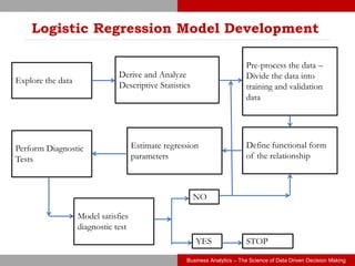
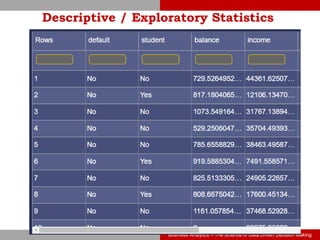
This document discusses logistic regression, a classification algorithm used to predict the probability of discrete outcomes. It provides examples of classification problems like customer churn, credit risk, fraud detection. Logistic regression models the log odds of the dependent variable using the sigmoid function. The document outlines the steps to develop a logistic regression model using a default prediction dataset: preprocessing data, fitting a model on training data, interpreting coefficients, assessing fit, making predictions on test data, and evaluating the model's performance.


![Business Analytics – The Science of Data Driven Decision Making
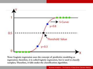
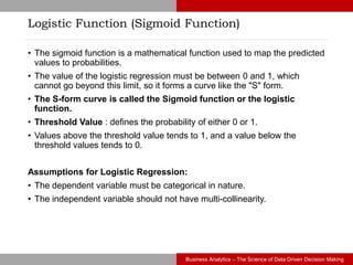
Logistic Function (Sigmoidal
function)
Logistic regression is a method used to fit a regression model when
the response variable is binary.
Logistic regression uses a method known as maximum likelihood
estimation to find an equation of the following form(Logistic
Function):
log(Y=1) =
log[p(X) / (1-p(X))] = β0 + β1X1 + β2X2 + … + βpXp
where:
Xj: The jth predictor variable(IV)
βj: The coefficient estimate for the jth predictor variable
The formula on the right side of the equation predicts the log
odds of the response variable (DV) taking on a value of 1.](https://image.slidesharecdn.com/chapter11logisticregression-221109031947-38857b03/85/CHAPTER-11-LOGISTIC-REGRESSION-pptx-7-320.jpg)