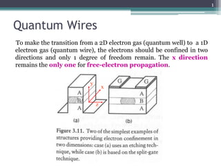
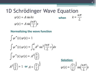
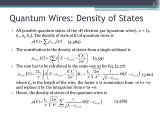
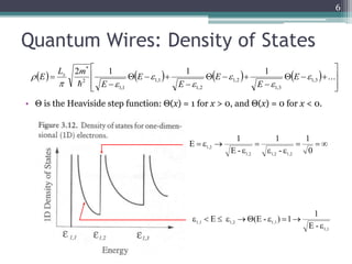
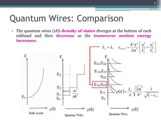
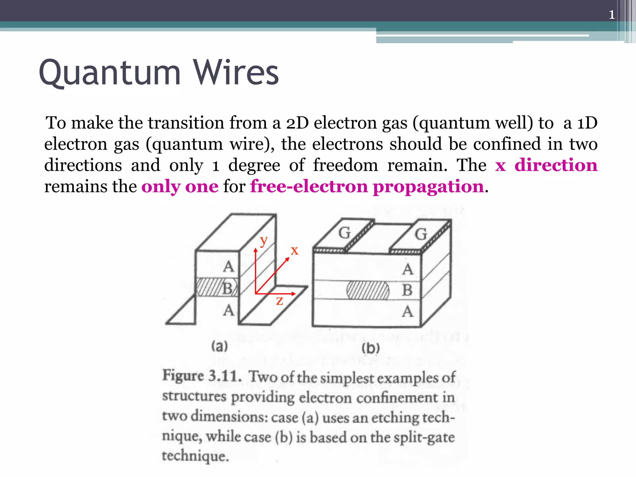
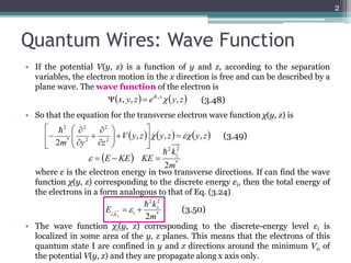
- The document discusses quantum wires and quantum dots. - For quantum wires, electrons are confined in two directions and free to move in the third, resulting in a 1D electron gas. The wave function and energy levels depend on the confinement potential. - For quantum dots, the potential confines electrons in all three dimensions, resulting in discrete energy levels. The wave function is a product of sine waves and the energy depends on quantum numbers in each dimension.

1. Quantum Wires
To make the transition from a 2D electron gas (quantum well) to a 1D
electron gas (quantum wire), the electrons should be confined in two
directions and only 1 degree of freedom remain. The x direction
remains the only one for free-electron propagation.
1
To make the transition from a 2D electron gas (quantum well) to a 1D electron gas
(quantum wire), the electrons should be confined in two directions and only 1 degree of
freedom remain. The x direction remains the only one for free-electron propagation.
x
y
z

2. Quantum Wires: Wave Function
• If the potential V(y, z) is a function of y and z, according to the separation
variables, the electron motion in the x direction is free and can be described by a
plane wave. The wave function of the electron is
• So that the equation for the transverse electron wave function χ(y, z) is
2
2






2
||
2
k
where ε is the electron energy in two transverse directions. If can find the wave
function χ(y, z) corresponding to the discrete energy εi, then the total energy of
the electrons in a form analogous to that of Eq. (3.24)
2 2
k

E x
  (3.50)
i k i x
• The wave function χi(y, z) corresponding to the discrete-energy level εi is
localized in some area of the y, z planes. This means that the electrons of this
quantum state I are confined in y and z directions around the minimum V0 of
the potential V(y, z) and they are propagate along x axis only.
2
x y z e y z  , ,  ikx x ,
Vy z y z y z
m y z
, , ,
2 *
2
2
2
 



  

 






(3.48)
(3.49)
  *
2m
E KE KE

   
*
, 2m

3. Quantum Wires: Energy Levels
• The simple case, in which the 2D SWE problem can be solved, is given by an
infinitely deep rectangular potential
y L z L
0 for 0 ,0
   
y z
, (3.51)
y z y L z L
where Ly and Lz are the transverse dimensions of the wires.
• For this case, the electron wave function χ(y, z) can be represented as a
product of functions depending separately on y and z.
(3.52)
• For each of the directions, solutions of the 1D SWE problem have the same
form of
2
n z
n y
and the quantized energy εi of the transverse motion of the electrons is
3

 


 
2
1
2 2
n

  2
n n L
1, 2 2 y z

2
2
2
*
n
L
m


 



    

y z
V y z
for 0, 0, ,
y z y z n1 n2  ,   
  sin
  sin , 1,2,3,...
2
1 2
2
2
1
1   n n 
L
L
z
L
L
y
z z
n
y y
n



 (3.53)
(3.54)

4. 1D Schrödinger Wave Equation
4
when
Normalizing the wave function
or
Solution:

5. Quantum Wires: Density of States
• All possible quantum states of the 1D electron gas (quantum wires), v = {s,
n1, n2, kx}. The density of state ρ(E) of quantum wires is
n n E E 1, 2   (3.58a)
• The contribution to the density of states from a single subband is


2 2

E E *
  
  
k
2
• The sum has to be calculated in the same way as for Eq. (3.27)
2 2
k


  
   
where Lx is the length of the wire, the factor 2 is summation from -∞ to +∞
and replace it by the integration from 0 to +∞.
• Hence, the density of states of the quantum wires is
5
    

 

kx
x
n 1, n 2 n 1, n 2 2
m
(3.60)
    
v
(3.58b)
(3.59)
    1, 2
1, 2
2
*
0
*
1, 2 1, 2
2 1
2
2
n n
n n
x
x
x
n n
x
n n E
E
L m
dk
m
E
L
E 
 
 


  

 




* 2 1
  x   E
 


1, 2
1, 2
1, 2
2
n n
n n
n n
E
L m
E 
 



6. Quantum Wires: Density of States

2m 1
L
(E) 1,3

1
1
2 1 1 1
 E

 ...


• Θ is the Heaviside step function: Θ(x) = 1 for x > 0, and Θ(x) = 0 for x < 0.
6
       





  

  

  

1,3
1,3
1,2
1,2
1,1
1,1
2
*





 
E
E
E
E
E
L m
E x

 is the Heaviside step function: (x) = 1 for x > 0, and (x) = 0 when x < 0.
(E - ) ....
E -
(E - )
E -
(E - )
E -
1,3
1,2
1,2
1,1
1,1
2
*
x
 

 

  

  

  
 
 

1
  
1
 


  
0
-
1
E -
E
1,2 1,2 1,2
1,2
1,1
1
E (E - ) 1
1,1 1,2 1,1 E -

       

7. Quantum Wires: Comparison
• The quantum wires (1D) density of states diverges at the bottom of each
subband and then decrease as the transverse motion energy
increases.
7







2
1
2 2
n
   2
x y n n L
1, 2 2 y z

2
2
2
*
n
L
m
L L



 
1,1
* 2 1
2
 



E
L m
E x
*
2 
m


8. Quantum Wires: Summary
• The wave function
n z
n y




 x  
y z   ik x
• The transverse motion energy
• The total energy


E x
• The density of states
8
2
1
2 2




n
n
  n n
1, 2 
m y z
2 2
2
2
2
1
n
n
 
* 2 1
2
2
2 2
k
  x   E
 


1, 2
1, 2
1, 2
2
n n
n n
n n
E
L m
E 
 


, 1,2,3,...
2 *
2
2 1 2




L
L
n n



*
2
2
*
1, 2, 2 m
L
L
2m
y z
n n kx
 








y y z z
e x
L
L L
L

 








 
 2
 1 sin
2 sin
2
, ,
x 1 for x  0, and x  0 when x  0.

9. Quantum Dots: Wave Functions and
Energy Levels
The confining potential in quantum dots is a function of all three coordinates and confines electrons in
all three directions. The simplest potential V(x,y,z) of this type is
• The confining potential in quantum dots is a function of all three
coordinates and confines electrons in all three directions. The simplest
potential V(x, y, V(z) x,of y,z) this type = 0 when is
inside the box
= + when outside the box
V x , y , z  0 when inside the box
(3.61)
where the box is restricted by the conditions 0  x  Lx, 0  y  Ly and 0  z  Lx.
where the box is restricted by the conditions 0≤x≤Lx, 0≤y≤Ly, 0≤z≤Lz.
The wave function after solving of SWE (Eq. 2.27) is
• The wave function after solving of SWE (Eq.2.27) is

πzn




πxn

n z
πyn
n y
n x
8
8
n n n L L L
L
L
L
• The total electron energy (no transverse confinement
like in quantum wells and quantum wires) is
9
 
when outside the box
 
   

 













 
x y z x y z
x y z
   1 2 3
, ,
sin sin sin
1, 2, 3 where , , 1,2,3,... 1 2 3 n n n 

2
1
 
n
(
2
3
2
2
2 2
E = 2


 
2
2
2
1
2 2
n
n
π
   2
n n n L
1, 2, 3 2 x y z

2
3
2
2
*
n
L
L
m
E
 
where , , 1,2,3,... 1 2 3 n n n 
(3.61)
)
L
) sin(
L
) sin(
L
sin(
L L L
ψ (x,y,z) =
z
3
y
2
x
1
x y z
n1,n2,n3
where n1, n2, n3 = 1, 2, 3, …
The total electron energy (no transverse confinement like in
quantum wells and quantum wires) is
)
n
+
L
n
+
L
L
2m
z
2
y
2
x
*
n1,n2,n3

where n1, n2, n3 = 1, 2, 3, …

10. Quantum Dots: Density of States
• The density of states from Eq. (3.26) is defined as
v  E  E E
• In the case of quantum dots, the density of states is simply a set of δ-shaped
peaks in idealized case, the peaks are very narrow and infinitely high due to
a single value of total energy (En1,n2,n3).


2
2
2
1
2 2
n
n
   2
n n n L
1, 2, 3 2 x y z
• Interactions between electrons and impurities as well as collisions with
phonons bring about a broadening of the discrete levels, as a result, the
peaks for physically realizable systems have finite amplitude and widths.
10
     
v
 

 

2
3
2
2
*
n
L
L
m
E
 

11. Quantum Dots: Density of States
• The energy spectra (E-k diagram) of the quantum box is completed, especially for
large number of quantum numbers. It is reasonable to estimate for the total number
of energy levels inside a quantum dot.
The energy spectra (E-k diagram) of the quantum box is complex, especially for large number of quantum
numbers. It is reasonable to estimates for the total number of energy levels inside a quantum dot.
• Refer to Eq. (3.28), the number of states (with spin) of 1D free motion in space
Refer to Eq. (3.28), the number of states (with spin) of 1D free motion in space region of length L in
the interval of wave vectors k is
region of length ΔL in the interval of wave vectors Δk is
• To generalize to 3D case:
2 1 L k D  
 
ΔL Δk
 D x y z xk yk zk
 
To generalize to 3D case :
Δx Δk ΔyΔk ΔzΔk
3D x y z
• Let consider an arbitrary potential V(x, y, z) < 0 (electron is bounded inside the
quantum dot). Fix a point of space r(x, y, z) and calculate the number of state
corresponding to the small volume ΔxΔyΔz around r.
Let consider an arbitrary potential V(x,y,z) < 0 (electron is bounded inside the quantum dot). Fix a point
of space r(x,y,z) and calculate the number of state corresponding to the small volume xyz around r.
• The possible values of the electron wave vector within the region of confinement
is
• Using semi-classical approach, for which the total energy is
2 2
k

0  k(r)  kmax(r) (3.77)
E   *
2 2 
• For bound states, E ≤ 0, then
11
kr k r max 0  


2
 3
3
2
2

(3.75)
(3.76)
(3.77)
Vr
m
2
 
k
E = *
 
m V r
2
*
max
2

k r 
2π
Δρ = 2 1D
3
(2π
Δρ = 2

(3.75)
(3.76)
z
y
r
x
y
z x
The possible values of the electron wave vector within the region of
confinement is
Using semi-classical approach, for which the total energy is
For bound states, E  0, then
+ V(r)
2m
(3.77)
2
*
max
2m V(r)
k (r) =

(3.78)

12. Quantum Dots: Density of States
• The integration over all possible k that satisfy relation in Eq. (3.77) gives the number
of states in the volume ΔxΔyΔz of
• By summing over of all classically allowed electron coordinates, the total number of
the energy states inside a quantum dots is found to be
m
3
3
*
2 2
 
• For a dot with potential given by Eq. (3.61) with a finite potential depth Vb, then the
total number of energy states is
m
3
3
*
2 2
 
 (3.81)
N 2
• The actual number of electrons inside the box is less than Nt. The amount of this
reduction is determined by the level of impurity doping.
• It is possible to control the number of the localized electrons by application of an
external field.
12
  Vr dxdydz
Nt
2
2 3
2
3
2
3
3 max
3

k x y z D   
  (3.79)
(3.80)
t b x y z V L L L
2 3
2
3

13. Quantum Dots: Comparison
13







2
2
2
1
L L L
x y z
2 2
n
n
  
n
1, 2, 3 2 x y z

 
2
3
2
2
2
*
n n n
L
L
L
m
E
 
 
1,1
* 2 1
2
 



E
L m
E x

*
2
m


14. Quantum Dots: Summary
• The wave function
• The total energy
• The density of states
14






n z
n y
n x
8
   
n n n L L L
L
2
2
2
1
2 2
n
n
   2
n n n L
1, 2, 3 2 x y z
m
3

3
*
2 2
 
N 2
t b x y z V L L L
2 3
2
3


 

 

2
3
2
2
*
n
L
L
m
E
 

 













 
L
L
x y z x y z
x y z
   1 2 3
, ,
sin sin sin
1, 2, 3 where , , 1,2,3,... 1 2 3 n n n 