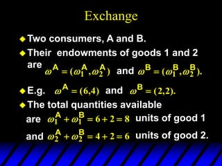
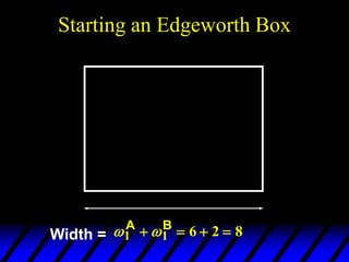
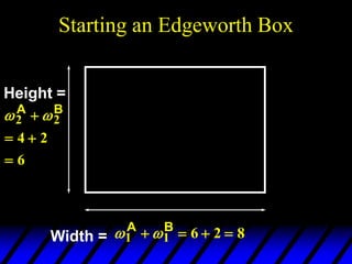
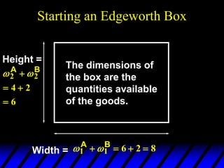
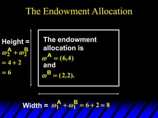
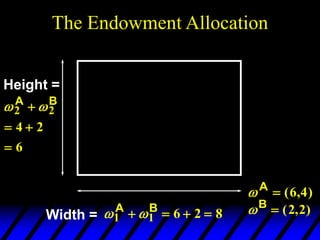
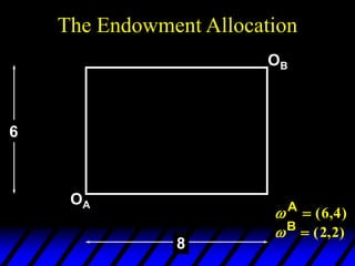
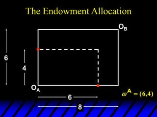
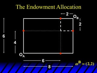
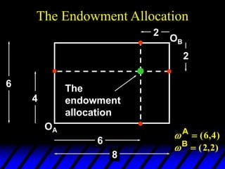
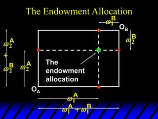
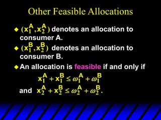
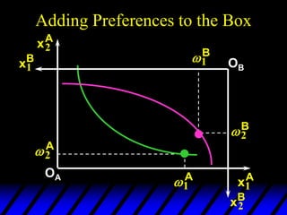
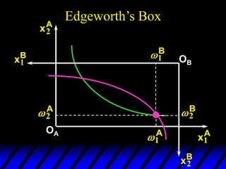
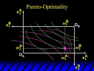
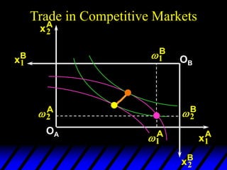
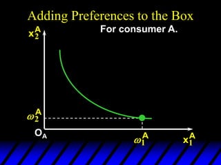
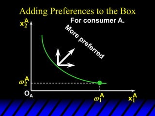
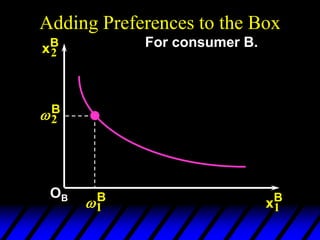
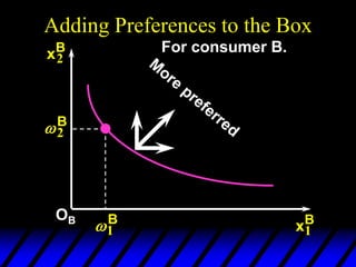
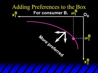
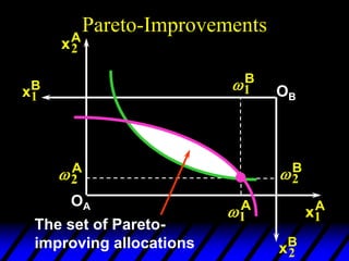
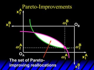
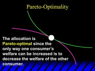
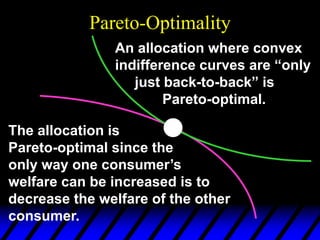
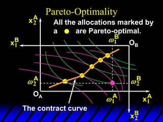
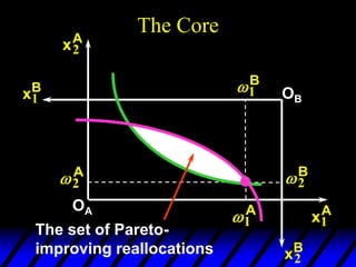
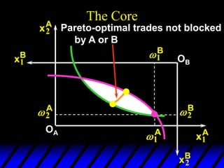
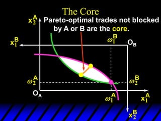
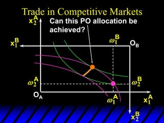
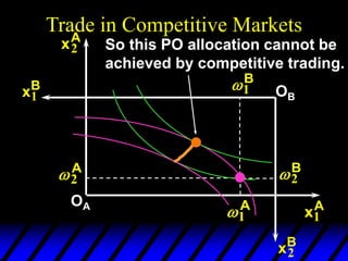
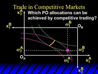
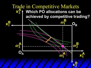
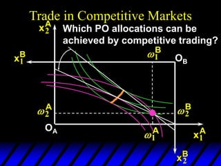
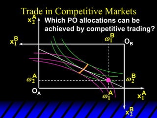
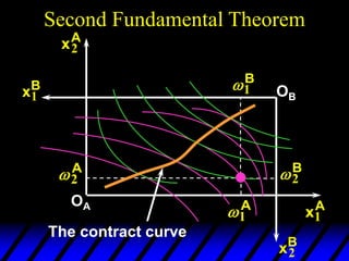
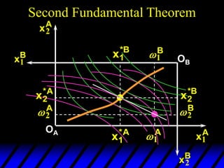
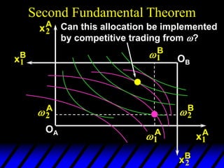
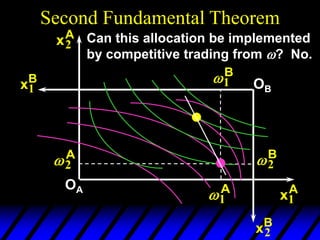
This document describes an Edgeworth box model of exchange between two consumers, A and B. It summarizes the key aspects of the model, including: 1) The endowments of goods 1 and 2 for each consumer define the dimensions of the Edgeworth box. All points within the box represent feasible allocations. 2) Pareto-improving allocations make at least one consumer better off without making the other worse off. The set of Pareto-optimal allocations form the contract curve. 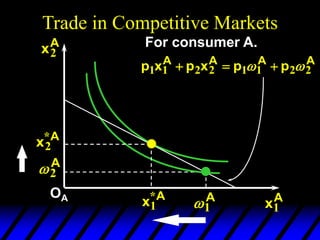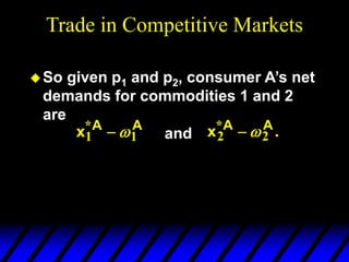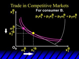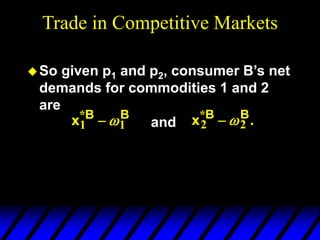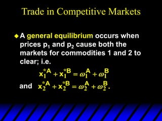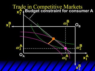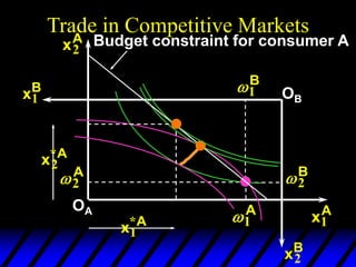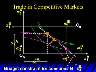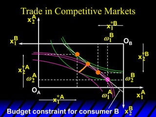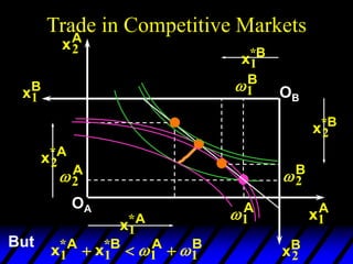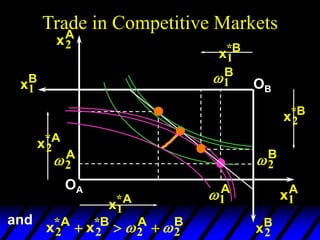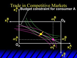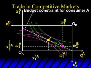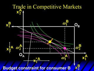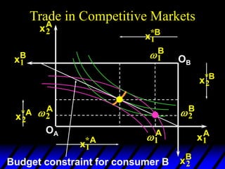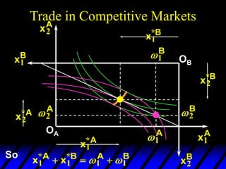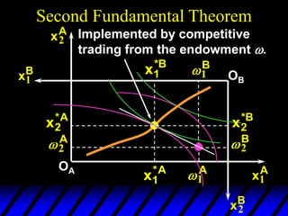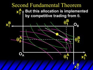3) In competitive markets, each consumer maximizes utility given market prices. General equilibrium occurs when resulting demands clear both markets. This determines a core allocation from trade.

1. Chapter Twenty-Nine
Exchange

2. Exchange
Two consumers, A and B.
Their endowments of goods 1 and 2
are
E.g.
The total quantities available
  
A A A
 ( , )
1 2   
B B B
 ( , ).
1 2
and
 A
 ( , )
6 4 B
 ( , ).
2 2
and
 
1 1 6 2 8
A B
   
 
2 2 4 2 6
A B
   
units of good 1
units of good 2.
and
are

3. Exchange
Edgeworth and Bowley devised a
diagram, called an Edgeworth box, to
show all possible allocations of the
available quantities of goods 1 and 2
between the two consumers.

4. Starting an Edgeworth Box

5. Starting an Edgeworth Box
Width =  
1 1 6 2 8
A B
   

6. Starting an Edgeworth Box
Width =  
1 1 6 2 8
A B
   
Height =
 
2 2
4 2
6
A B

 


7. Starting an Edgeworth Box
Width =  
1 1 6 2 8
A B
   
Height =
 
2 2
4 2
6
A B

 

The dimensions of
the box are the
quantities available
of the goods.

8. Feasible Allocations
What allocations of the 8 units of
good 1 and the 6 units of good 2 are
feasible?
How can all of the feasible
allocations be depicted by the
Edgeworth box diagram?

9. Feasible Allocations
What allocations of the 8 units of
good 1 and the 6 units of good 2 are
feasible?
How can all of the feasible
allocations be depicted by the
Edgeworth box diagram?
One feasible allocation is the before-
trade allocation; i.e. the endowment
allocation.

10. Width =  
1 1 6 2 8
A B
   
Height =
 
2 2
4 2
6
A B

 

The endowment
allocation is
 A
 ( , )
6 4
B
 ( , ).
2 2
and
The Endowment Allocation

11. Width =  
1 1 6 2 8
A B
   
Height =
 
2 2
4 2
6
A B

 

 A
 ( , )
6 4
B
 ( , )
2 2
The Endowment Allocation

12.  A
 ( , )
6 4
OA
OB
6
8
B
 ( , )
2 2
The Endowment Allocation

13.  A
 ( , )
6 4
OA
OB
6
8
4
6
The Endowment Allocation

14. B
 ( , )
2 2
OA
OB
6
8
4
6
2
2
The Endowment Allocation

15.  A
 ( , )
6 4
B
 ( , )
2 2
OA
OB
6
8
4
6
2
2
The
endowment
allocation
The Endowment Allocation

16. More generally, …
The Endowment Allocation

17. The Endowment Allocation
OA
OB
The
endowment
allocation
 
1 1
A B

2
A


2
2
A
B

1
A
1
B
2
B

18. Other Feasible Allocations
 denotes an allocation to
consumer A.
 denotes an allocation to
consumer B.
An allocation is feasible if and only if
( , )
x x
A A
1 2
( , )
x x
B B
1 2
x x
A B A B
1 1 1 1
  
 
x x
A B A B
2 2 2 2
  
  .
and

19. Feasible Reallocations
OA
OB
 
1 1
A B

xA
2


2
2
A
B

xA
1
xB
1
xB
2

20. Feasible Reallocations
OA
OB
 
1 1
A B

xA
2


2
2
A
B

xA
1
xB
1
xB
2

21. Feasible Reallocations
All points in the box, including the
boundary, represent feasible
allocations of the combined
endowments.

22. Feasible Reallocations
All points in the box, including the
boundary, represent feasible
allocations of the combined
endowments.
Which allocations will be blocked by
one or both consumers?
Which allocations make both
consumers better off?

23. Adding Preferences to the Box
2
A
1
A
xA
2
xA
1
OA
For consumer A.

24. Adding Preferences to the Box
2
A
1
A
xA
2
xA
1
For consumer A.
OA

25. Adding Preferences to the Box
2
B
1
B
xB
2
xB
1
For consumer B.
OB

26. Adding Preferences to the Box
xB
2
xB
1
For consumer B.
OB
2
B
1
B

27. Adding Preferences to the Box
2
B
1
B
xB
1
xB
2
For consumer B. OB

28. Adding Preferences to the Box
2
A
1
A
xA
2
xA
1
OA
For consumer A.

29. Adding Preferences to the Box
2
A
1
A
xA
2
xA
1
OA
2
B
1
B
xB
1
xB
2
OB

30. Edgeworth’s Box
2
A
1
A
xA
2
xA
1
OA
2
B
1
B
xB
1
xB
2
OB

31. Pareto-Improvement
An allocation of the endowment that
improves the welfare of a consumer
without reducing the welfare of
another is a Pareto-improving
allocation.
Where are the Pareto-improving
allocations?

32. Edgeworth’s Box
2
A
1
A
xA
2
xA
1
OA
2
B
1
B
xB
1
xB
2
OB

33. Pareto-Improvements
2
A
1
A
xA
2
xA
1
OA
2
B
1
B
xB
1
xB
2
OB
The set of Pareto-
improving allocations

34. Pareto-Improvements
Since each consumer can refuse to
trade, the only possible outcomes
from exchange are Pareto-improving
allocations.
But which particular Pareto-
improving allocation will be the
outcome of trade?

35. Pareto-Improvements
2
A
1
A
xA
2
xA
1
OA
2
B
1
B
xB
1
xB
2
OB
The set of Pareto-
improving reallocations

36. Pareto-Improvements

37. Pareto-Improvements

38. Pareto-Improvements
Trade
improves both
A’s and B’s welfares.
This is a Pareto-improvement
over the endowment allocation.

39. Pareto-Improvements
New mutual gains-to-trade region
is the set of all further Pareto-
improving
reallocations.
Trade
improves both
A’s and B’s welfares.
This is a Pareto-improvement
over the endowment allocation.

40. Pareto-Improvements
Further trade cannot improve
both A and B’s
welfares.

41. Pareto-Optimality
Better for
consumer B
Better for
consumer A

42. Pareto-Optimality
A is strictly better off
but B is strictly worse
off

43. Pareto-Optimality
A is strictly better off
but B is strictly worse
off
B is strictly better
off but A is strictly
worse off

44. Pareto-Optimality
A is strictly better off
but B is strictly worse
off
B is strictly better
off but A is strictly
worse off
Both A and
B are worse
off

45. Pareto-Optimality
A is strictly better off
but B is strictly worse
off
B is strictly better
off but A is strictly
worse off
Both A
and B are
worse
off
Both A and
B are worse
off

46. Pareto-Optimality
The allocation is
Pareto-optimal since the
only way one consumer’s
welfare can be increased is to
decrease the welfare of the other
consumer.

47. Pareto-Optimality
The allocation is
Pareto-optimal since the
only way one consumer’s
welfare can be increased is to
decrease the welfare of the other
consumer.
An allocation where convex
indifference curves are “only
just back-to-back” is
Pareto-optimal.

48. Pareto-Optimality
Where are all of the Pareto-optimal
allocations of the endowment?

49. Pareto-Optimality
2
A
1
A
xA
2
xA
1
OA
2
B
1
B
xB
1
xB
2
OB

50. Pareto-Optimality
2
A
1
A
xA
2
xA
1
OA
2
B
1
B
xB
1
xB
2
OB
All the allocations marked by
a are Pareto-optimal.

51. Pareto-Optimality
The contract curve is the set of all
Pareto-optimal allocations.

52. Pareto-Optimality
2
A
1
A
xA
2
xA
1
OA
2
B
1
B
xB
1
xB
2
OB
All the allocations marked by
a are Pareto-optimal.
The contract curve

53. Pareto-Optimality
But to which of the many allocations
on the contract curve will consumers
trade?
That depends upon how trade is
conducted.
In perfectly competitive markets? By
one-on-one bargaining?

54. The Core
2
A
1
A
xA
2
xA
1
OA
2
B
1
B
xB
1
xB
2
OB
The set of Pareto-
improving reallocations

55. The Core
2
A
1
A
xA
2
xA
1
OA
2
B
1
B
xB
1
xB
2
OB

56. The Core
2
A
1
A
xA
2
xA
1
OA
2
B
1
B
xB
1
xB
2
OB
Pareto-optimal trades blocked
by B
Pareto-optimal trades blocked
by A

57. The Core
2
A
1
A
xA
2
xA
1
OA
2
B
1
B
xB
1
xB
2
OB
Pareto-optimal trades not blocked
by A or B

58. The Core
2
A
1
A
xA
2
xA
1
OA
2
B
1
B
xB
1
xB
2
OB
Pareto-optimal trades not blocked
by A or B are the core.

59. The Core
The core is the set of all Pareto-
optimal allocations that are welfare-
improving for both consumers
relative to their own endowments.
Rational trade should achieve a core
allocation.

60. The Core
But which core allocation?
Again, that depends upon the
manner in which trade is conducted.

61. Trade in Competitive Markets
Consider trade in perfectly
competitive markets.
Each consumer is a price-taker trying
to maximize her own utility given p1,
p2 and her own endowment. That is,
...

62. Trade in Competitive Markets
2
A
1
A
xA
2
xA
1
OA
For consumer A.
p x p x p p
A A A A
1 1 2 2 1 1 2 2
  
 
x A
2
*
x A
1
*

63. Trade in Competitive Markets
So given p1 and p2, consumer A’s net
demands for commodities 1 and 2
are
x A A
1 1
*
  x A A
2 2
*
.
 
and

64. Trade in Competitive Markets
And, similarly, for consumer B …

65. Trade in Competitive Markets
2
B
1
B
xB
2
xB
1
For consumer B.
OB
x B
1
*
x B
2
*
p x p x p p
B B B B
1 1 2 2 1 1 2 2
  
 

66. Trade in Competitive Markets
So given p1 and p2, consumer B’s net
demands for commodities 1 and 2
are
x B B
1 1
*
  x B B
2 2
*
.
 
and

67. Trade in Competitive Markets
A general equilibrium occurs when
prices p1 and p2 cause both the
markets for commodities 1 and 2 to
clear; i.e.
x x
A B A B
1 1 1 1
* *
  
 
x x
A B A B
2 2 2 2
* *
.
  
 
and

68. Trade in Competitive Markets
2
A
1
A
xA
2
xA
1
OA
2
B
1
B
xB
1
xB
2
OB

69. Trade in Competitive Markets
2
A
1
A
xA
2
xA
1
OA
2
B
1
B
xB
1
xB
2
OB
Can this PO allocation be
achieved?

70. Trade in Competitive Markets
2
A
1
A
xA
2
xA
1
OA
2
B
1
B
xB
1
xB
2
OB
Budget constraint for consumer A

71. Trade in Competitive Markets
2
A
1
A
xA
2
xA
1
OA
2
B
1
B
xB
1
xB
2
OB
Budget constraint for consumer A
x A
2
*
x A
1
*

72. Trade in Competitive Markets
2
A
1
A
xA
2
xA
1
OA
2
B
1
B
xB
1
xB
2
OB
Budget constraint for consumer B
x A
2
*
x A
1
*

73. Trade in Competitive Markets
2
A
1
A
xA
2
xA
1
OA
2
B
1
B
xB
1
xB
2
OB
Budget constraint for consumer B
x A
2
*
x A
1
*
x B
1
*
x B
2
*

74. Trade in Competitive Markets
2
A
1
A
xA
2
xA
1
OA
2
B
1
B
xB
1
xB
2
OB
x A
2
*
x A
1
*
x B
1
*
x B
2
*
But
x x
A B A B
1 1 1 1
* *
  
 

75. Trade in Competitive Markets
2
A
1
A
xA
2
xA
1
OA
2
B
1
B
xB
1
xB
2
OB
x A
2
*
x A
1
*
x B
1
*
x B
2
*
and
x x
A B A B
2 2 2 2
* *
  
 

76. Trade in Competitive Markets
So at the given prices p1 and p2 there
is an
– excess supply of commodity 1
– excess demand for commodity 2.
Neither market clears so the prices
p1 and p2 do not cause a general
equilibrium.

77. Trade in Competitive Markets
2
A
1
A
xA
2
xA
1
OA
2
B
1
B
xB
1
xB
2
OB
So this PO allocation cannot be
achieved by competitive trading.

78. Trade in Competitive Markets
2
A
1
A
xA
2
xA
1
OA
2
B
1
B
xB
1
xB
2
OB
Which PO allocations can be
achieved by competitive trading?

79. Trade in Competitive Markets
Since there is an excess demand for
commodity 2, p2 will rise.
Since there is an excess supply of
commodity 1, p1 will fall.
The slope of the budget constraints
is - p1/p2 so the budget constraints
will pivot about the endowment point
and become less steep.

80. Trade in Competitive Markets
2
A
1
A
xA
2
xA
1
OA
2
B
1
B
xB
1
xB
2
OB
Which PO allocations can be
achieved by competitive trading?

81. Trade in Competitive Markets
2
A
1
A
xA
2
xA
1
OA
2
B
1
B
xB
1
xB
2
OB
Which PO allocations can be
achieved by competitive trading?

82. Trade in Competitive Markets
2
A
1
A
xA
2
xA
1
OA
2
B
1
B
xB
1
xB
2
OB
Which PO allocations can be
achieved by competitive trading?

83. Trade in Competitive Markets
2
A
1
A
xA
2
xA
1
OA
2
B
1
B
xB
1
xB
2
OB
Budget constraint for consumer A

84. Trade in Competitive Markets
2
A
1
A
xA
2
xA
1
OA
2
B
1
B
xB
1
xB
2
OB
Budget constraint for consumer A
x A
2
*
x A
1
*

85. Trade in Competitive Markets
2
A
1
A
xA
2
xA
1
OA
2
B
1
B
xB
1
xB
2
OB
Budget constraint for consumer B
x A
2
*
x A
1
*

86. Trade in Competitive Markets
2
A
1
A
xA
2
xA
1
OA
2
B
1
B
xB
1
xB
2
OB
Budget constraint for consumer B
x A
2
*
x A
1
*
x B
1
*
x B
2
*

87. Trade in Competitive Markets
2
A
1
A
xA
2
xA
1
OA
2
B
1
B
xB
1
xB
2
OB
x A
2
*
x A
1
*
x B
1
*
x B
2
*
So
x x
A B A B
1 1 1 1
* *
  
 

88. Trade in Competitive Markets
2
A
1
A
xA
2
xA
1
OA
2
B
1
B
xB
1
xB
2
OB
x A
2
*
x A
1
*
x B
1
*
x B
2
*
and
x x
A B A B
2 2 2 2
* *
  
 

89. Trade in Competitive Markets
At the new prices p1 and p2 both
markets clear; there is a general
equilibrium.
Trading in competitive markets
achieves a particular Pareto-optimal
allocation of the endowments.
This is an example of the First
Fundamental Theorem of Welfare
Economics.

90. First Fundamental Theorem of
Welfare Economics
Given that consumers’ preferences
are well-behaved, trading in perfectly
competitive markets implements a
Pareto-optimal allocation of the
economy’s endowment.

91. Second Fundamental Theorem of
Welfare Economics
The First Theorem is followed by a
second that states that any Pareto-
optimal allocation (i.e. any point on
the contract curve) can be achieved
by trading in competitive markets
provided that endowments are first
appropriately rearranged amongst
the consumers.

92. Given that consumers’ preferences
are well-behaved, for any Pareto-
optimal allocation there are prices
and an allocation of the total
endowment that makes the Pareto-
optimal allocation implementable by
trading in competitive markets.
Second Fundamental Theorem of
Welfare Economics

93. Second Fundamental Theorem
2
A
1
A
xA
2
xA
1
OA
2
B
1
B
xB
1
xB
2
OB
The contract curve

94. Second Fundamental Theorem
2
A
1
A
xA
2
xA
1
OA
2
B
1
B
xB
1
xB
2
OB
A
*
2
x B
*
2
x
A
*
1
x
B
*
1
x

95. Second Fundamental Theorem
2
A
1
A
xA
2
xA
1
OA
2
B
1
B
xB
1
xB
2
OB
A
*
2
x B
*
2
x
A
*
1
x
B
*
1
x
Implemented by competitive
trading from the endowment .

96. Second Fundamental Theorem
2
A
1
A
xA
2
xA
1
OA
2
B
1
B
xB
1
xB
2
OB
Can this allocation be implemented
by competitive trading from ?

97. Second Fundamental Theorem
2
A
1
A
xA
2
xA
1
OA
2
B
1
B
xB
1
xB
2
OB
Can this allocation be implemented
by competitive trading from ? No.

98. Second Fundamental Theorem
xA
2
xA
1
OA
xB
1
xB
2
OB
But this allocation is implemented
by competitive trading from q.
A
1
q
B
2
q
B
1
q
A
2
q

99. Walras’ Law
Walras’ Law is an identity; i.e. a
statement that is true for any
positive prices (p1,p2), whether these
are equilibrium prices or not.

100. Walras’ Law
Every consumer’s preferences are
well-behaved so, for any positive
prices (p1,p2), each consumer spends
all of his budget.
For consumer A:
For consumer B:
p x p x p p
A A A A
1 1 2 2 1 1 2 2
* *
  
 
p x p x p p
B B B B
1 1 2 2 1 1 2 2
* *
  
 

101. Walras’ Law
p x p x p p
A A A A
1 1 2 2 1 1 2 2
* *
  
 
p x p x p p
B B B B
1 1 2 2 1 1 2 2
* *
  
 
p x x p x x
p p
A B A B
A B B B
1 1 1 2 2 2
1 1 1 2 2 2
( ) ( )
( ) ( ).
* * * *
  
   
   
Summing gives

102. Walras’ Law
p x x p x x
p p
A B A B
A B B B
1 1 1 2 2 2
1 1 1 2 2 2
( ) ( )
( ) ( ).
* * * *
  
   
   
Rearranged,
p x x
p x x
A B A B
A B A B
1 1 1 1 1
2 2 2 2 2 0
( )
( ) .
* *
* *
   
   
 
 
That is, ...

103. Walras’ Law
.
0
)
x
x
(
p
)
x
x
(
p
B
2
A
2
B
*
2
A
*
2
2
B
1
A
1
B
*
1
A
*
1
1












This says that the summed market
value of excess demands is zero for
any positive prices p1 and p2 --
this is Walras’ Law.

104. Implications of Walras’ Law
0
)
x
x
(
p
)
x
x
(
p
B
2
A
2
B
*
2
A
*
2
2
B
1
A
1
B
*
1
A
*
1
1












Suppose the market for commodity A
is in equilibrium; that is,
.
0
x
x B
1
A
1
B
*
1
A
*
1 





Then
implies
.
0
x
x B
2
A
2
B
*
2
A
*
2 






105. Implications of Walras’ Law
So one implication of Walras’ Law for
a two-commodity exchange economy
is that if one market is in equilibrium
then the other market must also be in
equilibrium.

106. Implications of Walras’ Law
What if, for some positive prices p1 and
p2, there is an excess quantity supplied
of commodity 1? That is,
.
0
x
x B
1
A
1
B
*
1
A
*
1 





0
)
x
x
(
p
)
x
x
(
p
B
2
A
2
B
*
2
A
*
2
2
B
1
A
1
B
*
1
A
*
1
1












Then
implies
.
0
x
x B
2
A
2
B
*
2
A
*
2 






107. Implications of Walras’ Law
So a second implication of Walras’ Law
for a two-commodity exchange economy
is that an excess supply in one market
implies an excess demand in the other
market.