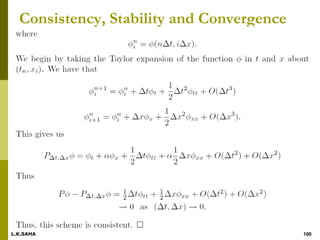
The document discusses consistency, stability, and convergence for finite difference approximations of partial differential equations (PDEs). It states that a finite difference approximation is consistent if the difference between the PDE and approximation goes to zero as the grid is refined. It is stable if errors do not grow from one time step to the next. Von Neumann stability analysis determines stability by examining the growth of Fourier components of the numerical solution.

1. Consistency, Stability and Convergence
L.K.SAHA 96
 Truncation Error
Consider the heat equation
Using a forward-difference representation for the time
derivative and a central difference representation for the space
derivative, and include the truncation errors associated with the
difference representation of the derivatives we obtain

2. Consistency, Stability and Convergence
L.K.SAHA 97
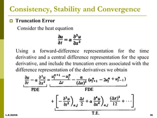
 truncation error for this finite-difference representation of the
heat equation is defined as the difference between the partial
differential equation and the difference approxi-mation to it.
That is, T.E. = PDE - FDE.
 The order of the truncation error in this case is O(t) + O[(x)2
] which is frequently expressed in the form O[t, (x)2 ].
Naturally, we solve only the finite-difference equations and
hope that the truncation error is small.
 How do we know that our difference representation is
acceptable and that a marching solution technique will work in
the sense of giving us an approximate solution to the PDE?
 In order to be acceptable, our difference representation for this
marching problem needs to meet the conditions of consistency
and stability.

3. Consistency, Stability and Convergence
L.K.SAHA 98
 A finite-difference representation of a PDE is said to be consistent if we can
show that the difference between the PDE and its difference representation
vanishes as the mesh is refined,
 This should always be the case if the order of the truncation error vanishes
under the grid refinement [i.e., O(t), O(x), etc.].
   
0 0
. . lim lim . 0
mesh mesh
i e PDE FDE T E
 
  

4. Consistency, Stability and Convergence
L.K.SAHA 99
 A finite difference approximation of a PDE is consistent if the finite
difference equation approaches the PDE as the grid size approaches zero.
 Given a partial differential equation Pu = f and a finite difference scheme,
Pt, x v = f, we say that the finite difference scheme is consistent with the
partial differential equation if for any smooth function (x, t)

5. Consistency, Stability and Convergence
L.K.SAHA 100

6. Consistency, Stability and Convergence
L.K.SAHA 102
 A stable numerical scheme is one for which errors from any
source (round-off, truncation, mistakes) are not permitted to
grow in the sequence of numerical procedures as the
calculation proceeds from one marching step to the next.
 Generally, concern over stability occupies much more of our
time and energy than does concern over consistency.
Consistency is relatively easy to check and most schemes
which are conceived will be consistent just due to the
methodology employed in their development.
 Stability is much more subtle and usually a bit of hard work is
required in order to establish analytically that a scheme is
stable.

7. Von Neumann Stability Analysis
L.K.SAHA 103
 Von Neumann stability analysis is a commonly used procedure
for determining the stability requirements of finite difference
equations.
 In this method, a solution of the finite difference equation is
expanded in a Fourier series. The decay or growth of the
amplification factor indicates whether or not the numerical
algorithm is stable.
 Recall that, for a linear equation, various solutions may be
added. Therefore, when the FDE under investigation is linear, it
is sufficient to investigate only one component of the Fourier
series. In fact, the linearity of the equation is a general
requirement for the application of the von Neumann stability
analysis. Furthermore, the effect of the boundary condition on
the stability of the solution is not included with this procedure.

8. Von Neumann Stability Analysis
L.K.SAHA 104
 To overcome these limitations, one may locally linearize the
nonlinear equation and subsequently apply the von Neumann
stability analysis.
 However, note that the resulting stability requirement is
satisfied locally. Therefore, the actual stability requirement
may be more restrictive than the one obtained from the von
Neumann stability analysis. Nevertheless, the results will
provide very useful information on stability requirements.
 To illustrate the procedure, assume a Fourier component for ui
n,
as