The document discusses key concepts in computer architecture including:
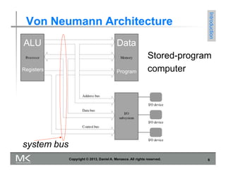
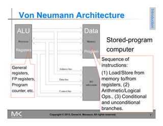
1) The Von Neumann architecture which defines the basic elements of a computer including the CPU, memory, and connection between them via a bus.
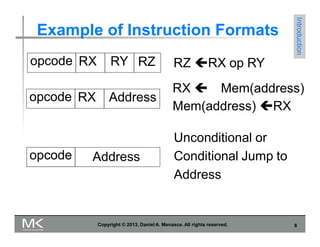
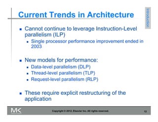
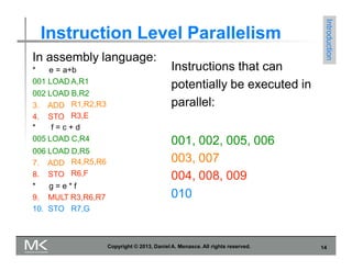
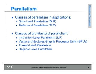
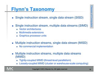
2) Different types of parallelism such as instruction-level, data-level, and task-level parallelism that have been exploited to improve performance.
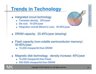
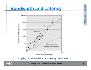
3) Trends that have driven computer performance over time, including improvements in semiconductor technology per Moore's Law, new architectures like RISC, and the shift to parallelism with multi-core processors.


![02 computer evolution and performance.ppt [compatibility mode]](https://cdn.slidesharecdn.com/ss_thumbnails/02computerevolutionandperformance-pptcompatibilitymode-120918022737-phpapp01-thumbnail.jpg?width=640&height=640&fit=bounds)


