บทที่ 1. ความสามารถเบื้องต้นของโปรแกรมMathcadMathcad – 4
8.4 สามารถเขียนกราฟแท่ง (Bar graph) ของข้อมูลทางสถิติ
ตัวอย่าง การเขียนกราฟของข้อมูล
คะแนน และ ความถี่
คะแนน ความถี่
1 15
2 35
3 40
4 10
8.5 สามารถเขียนกราฟในระบบพิกัดเชิงขั้ว
ตัวอย่าง การเขียนกราฟรูปหัวใจ r = 3 + 2sinθ, กราฟรูปกลีบกุหลาบ r = 4cos2θ
8.6 สามารถเขียนกราฟในระบบพิกัด 3 มิติ เช่นกราฟพื้นผิว กราฟ contour
ตัวอย่าง กราฟของพื้นผิวไฮเพอร์โบลิกพาราโบลอยด์
หรือพื้นผิวรูปอานม้า f(x, y) = 2
x – 2
y
ORIGIN 1:= i 1 4..:=
grade
1
2
3
4
:= frequency
15
35
40
10
:=
0 1 2 3 4 5
10
20
30
40
50
50
0
frequencyi
50 gradei
M M
i 1 20..:= j 1 20..:= xi 2− 0.2 i⋅+:= yj 2− 0.2 j⋅+:= f x y,( ) x
2
y
2
−:= M i j,( ) f xi yj,( ):=
θ 0 0.01, 2 π⋅..:=
0
30
60
90
120
150
180
210
240
270
300
330
5
4
3
2
1
0
3 2 sin θ( )⋅+
θ
0
30
60
90
120
150
180
210
240
270
300
330
5
4
3
2
1
0
4 cos 2 θ⋅( )⋅
θ
14.
บทที่ 1. ความสามารถเบื้องต้นของโปรแกรมMathcad Mathcaad – 5
8.7 สามารถปรับเปลี่ยนรูปแบบของกราฟให้เหมาะสมกับการใช้งาน
ตัวอย่าง กราฟของ f(x) = 3
x + 2
x – 9x – 9 บนช่วง [–4, 4]
แบบที่ 1. มีแกน X และแกน Y แต่ไม่มีสเกล แบบที่ 2. มีแกน X และแกน Y มีสเกล
แต่ไม่มีตัวเลขที่สเกล
แบบที่ 3. มีแกน X และแกน Y แบบที่ 4. มีแกน X และแกน Y
มีสเกลและมีตัวเลขที่สเกล มีสเกล มีตัวเลขที่สเกล
มีเส้นกริดช่วยในการประมาณค่า
8.8 สามารถเขียนกราฟ 2 ฟังก์ชันที่มีโดเมนต่างกันได้
ตัวอย่าง กราฟของ f(x) = 5 – 4x บนช่วง [–3, 1] และ g(t) = 2t + 10 บนช่วง [1, 4]
x 4− 3.99−, 4..:= f x( ) x
3
x
2
9 x⋅− 9−+:=
0
f x( )
x
x 4− 3.99−, 4..:= f x( ) x
3
x
2
9 x⋅− 9−+:=
f x( )
x
x 4− 3.99−, 4..:= f x( ) x
3
x
2
9 x⋅− 9−+:=
4 3 2 1 0 1 2 3 4
40
20
20
40
f x( )
x
x 3− 2.99−, 1..:= f x( ) 5 4 x⋅−:= t 1 1.01, 4..:= g t( ) 2 t⋅ 10+:=
4 3 2 1 0 1 2 3 4 5
5
5
10
15
20
f x( )
g t( )
x t,
.
x 4− 3.99−, 4..:= f x( ) x
3
x
2
+ 9 x⋅− 9−:=
4 3 2 1 0 1 2 3 4
40
20
20
40
f x( )
x
15.
บทที่ 1. ความสามารถเบื้องต้นของโปรแกรมMathcadMathcad – 6
9. การคํานวณในรูปแบบของเลขฐานอื่นๆ
ตัวอย่าง 12 ฐาน 8 บวกกับ 15 ฐาน 8 ได้ 23 ฐาน 10
12 ฐาน 16 บวกกับ 15 ฐาน 16 ได้ 39 ฐาน 10
หมายเหตุ อักษร o ท้ายตัวเลขหมายถึงเลขฐาน 8 และ อักษร h ท้ายตัวเลขหมายถึงเลขฐาน 16
10. การคํานวณในรูปแบบเวกเตอร์
Mathcad สามารถหาผลบวก ผลต่าง dot product cross product และ ขนาดของเวกเตอร์ได้
11. การคํานวณในรูปแบบเมทริกซ์
Mathcad สามารถหา ผลบวก ผลต่าง อินเวอร์ส ค่ากําหนด ของเมทริกซ์ได้
12. การคํานวณจํานวนเชิงซ้อน
Mathcad สามารถหาผลบวก ผลต่าง อินเวอร์ส ค่าสัมบูรณ์ของจํานวนเชิงซ้อนได้
13. การหาผลบวกในรูปแบบผลบวก ∑
ตัวอย่าง การหาผลบวกของตัวเลข
12o 15o+ 23=
12h 15h+ 39=
u
2
3
6
:= v
3
4
0
:=
u v+
5
7
6
= u v−
1−
1−
6
= u v×
24−
18
1−
= u v⋅ 18= u 7=
A
1
3
2
5
:= B
2
0
0
4
:= A B⋅
2
6
8
20
=
A B+
3
3
2
9
= 4 A⋅
4
12
8
20
= B 8= A 1−= A
1− 5−
3
2
1−
=
z 3 4i+:= w 5 12i+:=
z w+ 8 16i+= z w⋅ 33− 56i+= z 5= z
1−
0.12 0.16i−=
1
10
i
i∑
=
55=
1
10
i
i
2
∑
=
385=
1
10
i
i i 1+( )⋅∑
=
440=
16.
บทที่ 1. ความสามารถเบื้องต้นของโปรแกรมMathcad Mathcaad – 7
ตัวอย่าง การหาผลบวกของตัวแปร ix เมื่อ i = 1, 2, 3, ... , n
14. การคํานวณค่าสถิติเบื้องต้น
ตัวอย่าง การหาค่าสถิติเบื้องต้นของข้อมูล 2, 3, 7, 12, 16
mean = ค่าเฉลี่ย min = ค่าตํ่าสุด
median = มัธยฐาน max = ค่าสูงสุด
var = ความแปรปรวนของประชากร = n
)xx( 2
i
n
1i
−∑
=
stdev = ส่วนเบี่ยงเบนมาตรฐานของประชากร = )xvar(
Var = ความแปรปรวนของตัวอย่าง = 1n
)xx( 2
i
n
1i
−
−∑
=
Stdev = ส่วนเบี่ยงเบนมาตรฐานของตัวอย่าง = )x(Var
15. สามารถหาความสัมพันธ์เชิงฟังก์ชันของข้อมูลในรูปแบบ y = mx + c ได้
ตัวอย่าง การหาความสัมพันธ์เชิงเส้นตรงระหว่าง นํ้าหนัก (x) กับส่วนสูง (y)
นํ้าหนัก ความสูง
53 156
58 165
55 162
60 170
62 165
68 173
x เป็นตัวแปรอิสระ
y เป็นตัวแปรตาม
slope(x, y) คือ สัมประสิทธิ์การถดถอยเชิงเส้น
intercept(x, y) คือค่าคงตัวของสมการเส้นตรง y = mx + c
corr(x, y) คือ สัมประสิทธิ์สหสัมพันธ์เชิงเส้นตรง
ORIGIN 1:= i 1 5..:= xi
2
3
7
12
16
:=
1
5
i
xi∑
=
40=
1
5
i
xi( )2
∑
=
462=
ORIGIN 1:= i 1 5..:=
xi
2
3
7
12
16
:=
mean x( ) 8=
median x( ) 7=
stdev x( ) 5.329=
var x( ) 28.4=
Stdev x( ) 5.958=
Var x( ) 35.5=
max x( ) 16=
min x( ) 2=
ORIGIN 1:= i 1 6..:=
x
53
58
55
60
62
68
:= y
156
165
162
170
165
173
:=
m slope x y,( ):= m 0.995=
c intercept x y,( ):= c 106.109=
r corr x y,( ):= r 0.891=
17.
บทที่ 1. ความสามารถเบื้องต้นของโปรแกรมMathcadMathcad – 8
16. ความสามารถในการจัดรูปพีชคณิต การแยกตัวประกอบ การกระจายพหุนาม
16.1 การกระจายพหุนาม
ตัวอย่าง
16.2 การแยกตัวประกอบ
ตัวอย่าง
16.3 การจัดรูปแบบทางพีชคณิต
ตัวอย่าง
17. ความสามารถในการหาอนุพันธ์ และอนุพันธ์ย่อย ทั้งแบบค่าตัวเลขและเป็ นสูตร
17.1 การหาอนุพันธ์เป็นค่าตัวเลข
ตัวอย่าง การหาอนุพันธ์
ตัวอย่าง การหาอนุพันธ์ย่อย
17.2 การหาอนุพันธ์เป็นสูตร
ตัวอย่าง การหาอนุพันธ์
ตัวอย่าง การหาอนุพันธ์ย่อย
x 1−( ) x 2+( )⋅ expand x
2
x 2−+→
x 1+( ) x 2+( )
2
⋅ expand x
3
5 x
2
⋅+ 8 x⋅+ 4+→
x
2
5 x⋅+ 6+ factor x 3+( ) x 2+( )⋅→
x
3
5 x
2
⋅+ 8 x⋅+ 4+ factor x 1+( ) x 2+( )
2
⋅→
1
2
2
3
+ factor
7
6
→
1
1 2+
factor 2 1−→
1
1 x−
1
1 x+
+ factor
2−
x 1−( ) x 1+( )⋅[ ]
→
x 1:= f x( ) x
3
4 x
2
⋅+ 5 x⋅+ 4−:=
f x( ) 6=
x
f x( )
d
d
16=
2
x
f x( )
d
d
2
14=
3
x
f x( )
d
d
3
6=
x 2:= y 1:=
x
x
3
2 x
2
⋅ y⋅+ y
4
+( )d
d
20=
y y
x
3
2 x
2
⋅ y⋅+ y
4
+( )d
d
d
d
12=
x
x
3
4 x
2
⋅+ 5 x⋅+ 4−( )d
d
expand 3 x
2
⋅ 8 x⋅+ 5+→
2
x
x
3
4 x
2
⋅+ 5 x⋅+ 4−( )d
d
2
expand 6 x⋅ 8+→
x
x
3
2 x
2
⋅ y⋅+ y
4
+( )d
d
simplify 3 x
2
⋅ 4 x⋅ y⋅+→
y y
x
3
2 x
2
⋅ y⋅+ y
4
+( )d
d
d
d
simplify 12 y
2
⋅→
18.
บทที่ 1. ความสามารถเบื้องต้นของโปรแกรมMathcad Mathcaad – 9
18. ความสามารถในการหาปริพันธ์เป็ นสูตรและค่าตัวเลข
18.1 การหาปริพันธ์เป็นค่าตัวเลข
18.2 การหาปริพันธ์เป็นสูตร
19. สามารถหาค่าลิมิตได้
20. ความสามารถในการคํานวณเป็ นโปรแกรม
ตัวอย่าง โปรแกรมหาพื้นที่สามเหลี่ยมเมื่อรู้ความยาวทั้งสามด้าน
0
2
xx
3
1+( )⌠
⌡
d 6=
0
1
y
0
2
xx
3
y( )⌠
⌡
d
⌠
⌡
d 2=
0
1
z
1
2
y
1−
1
xx y
3
⋅ z+( )⌠
⌡
d
⌠
⌡
d
⌠
⌡
d 1=
xx
3
1+( )⌠
⌡
d simplify
1
4
x
4
⋅ x+→
yxx
3
y⋅( )⌠
⌡
d
⌠
⌡
d simplify
1
8
x
4
⋅ y
2
⋅→
zyxx y
3
⋅ z+( )⌠
⌡
d
⌠
⌡
d
⌠
⌡
d simplify
1
8
x
2
⋅ y
4
⋅ z⋅
1
2
z
2
⋅ x⋅ y⋅+→
1x
x
2
x+ 1+lim
→
3→
1x
x
2
1−
x 1−
lim
→
2→
0x
sin x( )
x
lim
→
1→
0x
x
x
lim
+→
1→
0x
x
x
lim
−→
1−→
∞x
1
1
x
+
2 x⋅
lim
→
exp 2( )→
a 3:=
b 4:=
c 5:=
s
a b+ c+
2
:=
Area s s a−( )⋅ s b−( )⋅ s c−( )⋅:=
Area 6=
1
x
2
t4 t
3
⋅ 1+( )⌠
⌡
d x
8
x
2
2−+→
1
t
y
0
t
2
x2x 4 y⋅+( )
⌠
⌡
d
⌠
⌡
d t
5
t
4
2 t
2
⋅−+→
19.
บทที่ 1. ความสามารถเบื้องต้นของโปรแกรมMathcadMathcad – 10
เมื่อเปลี่ยนค่า a, b, c ใหม่จะได้ผลการคํานวณเป็นดังนี้
21. ความสามารถในการหารากของสมการ f(x) = 0
ตัวอย่าง การหารากของสมการ 2
x - 2 = 0
เพราะฉะนั้นรากของสมการ
คือ x = 1.414 และ –1.414
ตัวอย่าง การหารากของสมการ sinx - cosx = 0
รากสมการ sinx - cosx = 0 คือ x = 0.785 radian หรือ 45 degree
22. ความสามารถในการหาผลเฉลยของระบบสมการ
22.1 การหาผลเฉลยของระบบสมการเชิงเส้น
ตัวอย่าง การหาผลเฉลยของระบบสมการ
2x + y = 4
9x – 4y = 1
เพราะฉะนั้น x = 1, y = 2
22.2 การหาผลเฉลยของระบบสมการไม่เชิงเส้น
ตัวอย่าง การหาผลเฉลยของระบบสมการ
2
x + 2
y = 1
และ x – y = 0
เพราะฉะนั้น x = 0.707, y = 0.707
23. ความสามารถในการหาผลเฉลยของสมการเชิงอนุพันธ์
ตัวอย่าง การหาผลเฉลยของสมการเชิงอนุพันธ์
dx
dy
= 1 + 4x, y(0) = 1
โปรแกรม Mathcad จะสามารถหาผลเฉลย y(x) ได้
ความสามารถอื่น ๆ ในการประยุกต์
เนื้อหาคณิตศาสตร์ขอให้ศึกษาในบทต่อไป
x 1:= root x
2
2− x,( ) 1.414=
x 1−:= root x
2
2− x,( ) 1.414−=
x 0:= y 0:=
Given
2 x⋅ y+ 4
9x 4 y⋅− 1
Find x y,( )
1
2
=
x 0:= y 0:=
Given
x
2
y
2
+ 1
x y− 0
Find x y,( )
0.707
0.707
=
x 1:= root sin x( ) cos x( )− x,( ) 45deg=
root sin x( ) cos x( )− x,( ) 0.785rad=
a 5:=
b 12:=
c 13:=
s
a b+ c+
2
:=
Area s s a−( )⋅ s b−( )⋅ s c−( )⋅:=
Area 30=
Given
x
y x( )
d
d
1 4 x⋅+ y 0( ) 1 .
y Odesolve x 10,( ):=
0 1 2 3 4
8
16
24
32
40
y x( )
x
y 1( ) 4= .
y 2( ) 11=
บทที่ 2. การใช้โปรแกรมสําเร็จรูปMathcad Mathcad - 29
2.8 การคํานวณค่าเกี่ยวกับผลบวกในรูปแบบ ∑
ตัวอย่าง การหาค่าของ ∑
=
10
1i
i , ∑
=
10
1i
2
i , (i2
− −
=
∑ 4 5
1
10
i
i
)
ขั้นตอนการนําแถบเครื่องมือคํานวณขึ้นมาใช้งาน
ขั้นที่ 1. เลือกเมนู View
ขั้นที่ 2. เลื่อนมาที่ Toolbars
ขั้นที่ 3. เลื่อนเมาส์มาที่ Math
ขั้นที่ 4. คลิกเมาส์ที่คําสั่ง Math
จะได้แถบเครื่องมือของการคํานวณ Math
ขั้นที่ 5. คลิกเมาส์ที่ Icon จะได้แถบเครื่องมือของ Calculus
หมายเหตุ การเข้ามาใช้งานโปรแกรม Mathcad
ในบางครั้งอาจมีแถบเครื่องมือของการคํานวณต่าง ๆ ปรากฏอยู่บนจอภาพแล้ว
การหาค่าของ ∑
=
10
1i
i , ∑
=
10
1i
2
i , (i2
− −
=
∑ 4 5
1
10
i
i
)
พิมพ์ ผลบนจอภาพ
การหาผลบวก ∑
=
10
1i
i
คลิกที่สัญลักษณ์
จะได้แถบเครื่องมือดังนี้
คลิกที่สัญลักษณ์
i<Tab>
i<Tab>
39.
บทที่ 2. การใช้โปรแกรมสําเร็จรูปMathcadMathcad - 30
1<Tab>
10=↵
1
10
i
i∑
=
55=
ในทํานองเดียวกันจะได้ว่า
2.9 การคํานวณค่าปริพันธ์ dx)x(f
b
a
∫ ตัวอย่างการหาค่าของ dxx
2
1
0
∫
พิมพ์ ผลบนจอภาพ
จากแถบเครื่องมือ Calculus
คลิกที่สัญลักษณ์
x^2<Tab>
x<Tab>
0<Tab>
1=↵
0
1
xx
2⌠
⌡
d 0.333=
1
10
i
i
2
∑
=
385=
1
10
i
i
2
4 i⋅− 5−( )∑
=
115=
40.
บทที่ 2. การใช้โปรแกรมสําเร็จรูปMathcad Mathcad - 31
หมายเหตุ ในกรณีที่เรากําหนด f(x) = 2
x จะทําให้การคํานวณสะดวกขึ้นดังนี้
2.10 การคํานวณค่าอนุพันธ์ )x(f
dx
d หรือ )x(f
dx
d
n
n
ตัวอย่าง การคํานวณ )x(f
dx
d เมื่อ f(x) = 2x ที่ x = 1
พิมพ์ ผลบนจอภาพ
f(x):x^2↵ f x( ) x
2
:=
x:1↵ x 1:=
จากแถบเครื่องมือ Calculus
คลิกที่สัญลักษณ์
x<Tab>
f(x)=↵
x
f x( )
d
d
2=
การคํานวณ )x(f
dx
d
2
2
เมื่อ f(x) = 4x ที่ x = 2
พิมพ์ ผลบนจอภาพ
f(x):x^4↵ f x( ) x
4
:= .
x:2↵ x 2:= .
จากแถบเครื่องมือ Calculus
คลิกที่สัญลักษณ์
f x( ) x
2
:=
0
1
xf x( )
⌠
⌡
d 0.333=
3−
3
xf x( )
⌠
⌡
d 18=
0
3
xf x( )
⌠
⌡
d 9=
41.
บทที่ 2. การใช้โปรแกรมสําเร็จรูปMathcadMathcad - 32
f(x)<Tab>
x<Tab>
2=↵
2
x
f x( )
d
d
2
48=
หมายเหตุ 1. กดเครื่องหมาย ? บนแป้ นพิมพ์จะได้สัญลักษณ์
2. กด <Ctrl> + ? บนแป้ นพิมพ์จะได้สัญลักษณ์
2.11 การกําหนดหน่วยให้กับผลการคํานวณ
พิมพ์ ผลบนจอภาพ
sin(30)=↵ sin 30( ) 0.988−=
หมายเหตุ ขณะนี้คอมพิวเตอร์จะคิดเป็นหน่วย เรเดียน
sin(30*deg)=↵ sin 30 deg⋅( ) 0.5=
หมายเหตุ 30.deg คือ 30 องศา
atan(1)=
หมายเหตุ ขณะนี้ผลลัพธ์มีหน่วยเป็น เรเดียน
<Tab>
d
eg↵ atan 1( ) 45deg=
ในทํานองเดียวกัน
2.12 การคํานวณในรูปแบบของเลขฐานอื่นๆ
ตัวอย่าง 12o + 17o = 25 o หมายถึงเลขฐาน 8
(12o)(11o) =
10h + 12h = 34 h หมายถึงเลขฐาน 16
(2h)(11h) = 32
cos 30( ) 0.154= cos 30 deg⋅( ) 0.866= asin 1( ) 1.571= asin 1( ) 90deg= .
s 1000 m⋅:= t 5 sec⋅:=
s
t
200
m
s
=
s 60 km⋅:= t 2 min⋅:=
s
t
500
m
s
=
s
t
30
km
min
=
42.
บทที่ 2. การใช้โปรแกรมสําเร็จรูปMathcad Mathcad - 33
พิมพ์ ผลบนจอภาพ
12o+17o=↵ 12o 17o+ 25=
หมายเหตุ 12 ฐาน 8 บวก 17 ฐาน 8 ได้ 25 ฐาน 10
12o*11o=↵ 12o 11o⋅ 90=
หมายเหตุ 10 ฐาน 8 คูณ 11 ฐาน 8 ได้ 90 ฐาน 10
10h+12h=↵ 10h 12h+ 34=
หมายเหตุ 10 ฐาน 16 บวก 12 ฐาน 16 ได้ 34 ฐาน 10
2h*11h=↵ 2h 10h⋅ 32=
หมายเหตุ 2 ฐาน 16 คูณ 11 ฐาน 16 ได้ 32 ฐาน 10
2.13 การหาผลบวกในรูปแบบ ∑
=
n
1i
ix
ตัวอย่างเช่น
พิมพ์ ผลบนจอภาพ
ORIGIN:1↵ ORIGIN 1:=
กําหนดเมทริกซ์ x และ y
การกําหนดเมทริกซ์ x และ y
ดูที่หัวข้อ 2.6
x
2
3
6
9
:= y
12
15
14
19
:=
การพิมพ์เพื่อหาผลบวก
จากแถบเครื่องมือ Calculus
คลิกที่สัญลักษณ์
ORIGIN 1:= x
2
3
6
9
:= y
12
15
14
19
:=
1
4
i
x
i∑
=
20=
1
4
i
y
i∑
=
60=
1
4
i
x
i( )2
∑
=
130=
1
4
i
y
i( )2
∑
=
926=
1
4
i
x
i
y
i
⋅∑
=
324=
บทที่ 2. การใช้โปรแกรมสําเร็จรูปMathcad Mathcad - 35
1<Tab>
4=↵
1
4
i
x
i( )2
∑
=
130=
การพิมพ์เพื่อหาผลบวก ii
4
1i
yx∑
=
คลิกที่สัญลักษณ์
x[i
<Space Bar>
*
y[i<Tab>
i<Tab>
1<Tab>
4=↵
1
4
i
x
i
y
i
⋅∑
=
324=
45.
บทที่ 2. การใช้โปรแกรมสําเร็จรูปMathcadMathcad - 36
2.14 การสร้างตารางฟังก์ชัน
การสร้างตารางฟังก์ชันมีขั้นตอนที่สําคัญดังต่อไปนี้
ขั้นที่ 1. กําหนดช่วงของตัวแปร x
ขั้นที่ 2. กําหนดสูตรของฟังก์ชัน f(x)
ขั้นที่ 3. พิมพ์ค่าของ x และ f(x)
ตัวอย่างเช่น
พิมพ์ ผลบนจอภาพ
x:1;4↵ x 1 4..:= .
f(x):2*x+4↵ f x( ) 2 x⋅ 4+:= .
x=↵ x
1
2
3
4
=
f(x)=↵ f x( )
6
8
10
12
=
หมายเหตุ ในกรณีที่ค่า x เพิ่มไม่เท่ากันสามารถคํานวณในรูปแบบตารางได้ดังนี้
2.15 การคํานวณค่าเกี่ยวกับจํานวนเชิงซ้อน
ตัวอย่าง (3 + 4i) + (5 - 9i) = 8 - 5i
| 3 + 4i | = 5
พิมพ์ ผลบนจอภาพ
z : 3+4i↵ z 3 4i+:= .
w : 5-9i↵ w 5 9i−:= .
x 1 4..:=
f x( ) 2 x⋅ 4+:=
x
1
2
3
4
= f x( )
6
8
10
12
=
x
2
5
7
12
:= f x( ) 2 x⋅ 4+:= f x( )
8
14
18
28
=
46.
บทที่ 2. การใช้โปรแกรมสําเร็จรูปMathcad Mathcad - 37
z+w=↵ z w+ 8 5i−=
|
z=↵ z 5=
2.16 การหารากของสมการ f(x) = 0
ตัวอย่าง การหารากของสมการ 2
x - 2 = 0
พิมพ์ ผลบนจอภาพ
f(x):x^2
<Space Bar>
-2↵ f x( ) x
2
2−:= .
x:1↵ x 1:= .
root(f(x), x)=↵ root f x( ) x,( ) 1.414= .
หมายเหตุ คําสั่ง root เป็นคําสั่งที่ใช้หารากของสมการ f(x) = 0 โดยวีธีของนิวตัน
โดยกําหนดจุดเริ่มต้นของการหารากที่ x = 1
ตัวอย่างการหารากของสมการอื่น ๆ เช่น
2.17 การผลเฉลยของระบบสมการ
ตัวอย่าง การหาผลเฉลยของระบบสมการ 2x + 3y = 8
x + y = 3
พิมพ์ ผลบนจอภาพ
x:0↵ x 0:= .
y:0↵ y 0:= .
Given↵ Given .
2*x+3*y
<Ctrl>+=
หมายเหต◌ุ กด <Ctrl>+= จึงจะได้สัญลักษณ์ = ที่มีสีดํา
เข้ม ตามรูปแบบของชุดคําสั่ง Given
8↵ 2 x⋅ 3y+ 8
x+y↵
f x( ) x
2
x− 20−:=
x 1:= root f x( ) x,( ) 5=
x 2−:= root f x( ) x,( ) 4−=
47.
บทที่ 2. การใช้โปรแกรมสําเร็จรูปMathcadMathcad - 38
<Ctrl>+=
3↵ x y+ 3
Find(x, y)=↵ Find x y,( )
1
2
=
หมายเหตุ ชุดคําสั่ง Given และ Find เป็นคําสั่งที่ใช้หาผลเฉลยของระบบสมการด้วยวิธีของนิวตัน
โดยกําหนดจุดเริ่มต้นของการหาผลเฉลย x = 0 และ y = 0
ตัวอย่าง การหาผลเฉลยของระบบสมการไม่เชิงเส้น
การหาจุดตัดของวงกลม 2
x + 2
y = 25
และเส้นตรง 3x + 4y = 0
2.18 การคํานวณค่า r
n
C และ r
n
P
สูตร r
n
C = )!rn(!r
!n
−
สามารถกําหนดเป็นสูตรในโปรแกรม Mathcad ได้ดังนี้
พิมพ์ ผลบนจอภาพ
C(n, r):n!
/
r!*
(n-r)!↵ C n r,( )
n!
r! n r−( )!⋅
:=
C(5, 1)= ↵ C 5 1,( ) 5=
C(5, 2)= ↵ C 5 2,( ) 10=
การกําหนดสูตร r
n
P = )!rn(
!n
−
P(n, r):
/
(n-r)!↵ P n r,( )
n!
n r−( )!
:=
P(5, 1)= ↵ P 5 1,( ) 5=
P(5, 2)= ↵ P 5 2,( ) 20=
x 1:= y 1:=
Given
x
2
y
2
+ 25 3x 4y+ 0 .
Find x y,( )
4
3−
=
48.
บทที่ 2. การใช้โปรแกรมสําเร็จรูปMathcad Mathcad - 39
ตัวอย่างการคํานวณในรูปแบบตาราง
2.19 การคํานวณที่ให้ผลลัพธ์เป็ นสูตร
โปรแกรม Mathcad สามารถคํานวณและแสดงผลออกมาในรูปแบบของสูตรได้เช่น
การกระจายพหุนาม (x - 1)(x + 2) กระจายได้เป็น 2
x + x - 2
การแยกตัวประกอบ 4
x - 2 2
x - 3x - 2 แยกตัวประกอบได้เป็น (x - 2)(x + 1)( 2
x + x + 1)
การแสดงผลเป็นเศษส่วนอย่างตํ่า
15
11
12
5
4
3
+
จัดรูปเป็น 23
15
การหาอนุพันธ์เป็นสูตร dx
d 2
x ผลการหาอนุพันธ์คือ 2x
การหาปริพันธ์เป็นสูตร dx)7x4( +∫ ผลการคํานวณเป็นสูตรคือ 2 2
x + 7x
สามารถหาค่าลิมิตได้
1x
lim
→
( 2
x + 2x + 4) หาค่าลิมิตได้เป็น 7
การคํานวณเพื่อให้โปรแกรม Mathcad แสดงผลเป็นสูตร มีขั้นตอนดังนี้
1. พิมพ์สูตรที่ต้องการคํานวณให้เรียบร้อย
2. ใช้การกด <Space bar> เพื่อขยาย curser ให้คลุมบริเวณสูตร การลดขนาด curser ที่คลุมสูตรให้กด ↓
หรือใช้การลากเมาส์เข้ามาคลุมบริเวณที่ต้องการผลการคํานวณเป็นสูตร
3. เลือกคําสั่งให้โปรแกรม Mathcad แสดงผลเป็นสูตร
ตัวอย่าง การกระจายสูตรพหุนาม (x - 1)(x + 2)
พิมพ์ ผลบนจอภาพ
(x-1)*(x+2)↵
<Space bar>
คลิก บนแถบเมนู จะได้เมนูย่อยเป็น
คลิก บนแถบเมนู x
2
x 2−+
หมายเหตุ หลังจากเลือกบริเวณสูตรแล้ว การสั่งอีกแบบทําได้โดยการกด <Alt>+s ค้างไว้ แล้วกด x
r 0 4..:= r
0
1
2
3
4
= C 4 r,( )
1
4
6
4
1
= P 4 r,( )
1
4
12
24
24
=
บทที่ 3. การเขียนกราฟด้วยMathcadMathcad – 52
การ Format รูปแบบกราฟให้มีลักษณะต่าง ๆ มีขั้นตอนดังนี้
พิมพ์ ผลบนจอภาพ
เลือกรูปของกราฟที่ต้องการ
เปลี่ยนรูปแบบ โดยการนําเมาส์
ไปคลิกที่บริเวณของกราฟ
จะเกิดกรอบคลุมบริเวณกราฟ
คลิก Format ที่เมนูบาร์
เลือกเมนูย่อย Graph
เลือกเมนูย่อย X-Y Plot
จะได้เมนูของการ Format กราฟดังนี้
หมายเหตุ วิธีที่สะดวกที่สุดในการ Format กราฟคือ กดดับเบิลคลิก ในบริเวณกราฟที่เราต้องการจัดรูปแบบ
เมนูย่อยที่มีคือ X-Y Axes เมนูย่อยเกี่ยวกับลักษณะของกรอบ และ สเกล
Traces เมนูย่อยเกี่ยวกับลักษณะของเส้นกราฟ สีของกราฟ การพล็อตจุด
Labels เมนูย่อยเกี่ยวกับการพิมพ์ชื่อของ แกน X แกน Y
Defaults เมนูย่อยของการกําหนดค่ามาตรฐานของการเขียนกราฟ
X-Y Axes เมนูย่อยของการจัดรูปแบบเกี่ยวกับแกนพิกัด
Log Scale ใช้กําหนดว่าแกน X หรือ แกน Y เป็นสเกล log
Grids Lines ใช้กําหนดว่าต้องการตีเส้น grid หรือไม่
Numbered ใช้กําหนดว่าต้องการพิมพ์ตัวเลขที่แกน X หรือ แกน Y หรือไม่
Autoscale ใช้กําหนดว่าต้องการในคอมพิวเตอร์คํานวณสเกลให้หรือไม่
Show Markers ใช้กําหนดว่าต้องการให้พิมพ์สัญลักษณ์ที่ Plot กราฟหรือไม่
Auto Grid ใช้กําหนดว่าต้องการกําหนดจํานวน grid เองหรือไม่
62.
บทที่ 3. การเขียนกราฟด้วยMathcad Mathcad – 53
◌ฺBoxed ใช้กําหนดว่าต้องการเขียนกราฟในกรอบสี่เหลี่ยม
Crossed ใช้กําหนดว่าต้องการเขียนกราฟโดยไม่มีกรอบสี่เหลี่ยมล้อมรอบ
None เป็นการกําหนดว่าไม่ต้องเขียนแกน X และ แกน Y
หมายเหตุ มีเครื่องหมาย ถูก ในช่องสี่เหลี่ยมแปลว่าต้องการเลือก Option นั้น
Traces เมนูย่อยของการจัดรูปแบบ
เกี่ยวกับการพล็อตจุดของกราฟ
Legend Label ใช้แสดงหมายเลขเส้นกราฟ
Symbol ใช้กําหนดสัญลักษณ์ในการเขียนจุด
เช่นใช้เครื่องหมาย +, x
Line ใช้กําหนดชนิดของเส้นกราฟ
เป็นเส้บทึบ เส้นปะ
Color ใช้กําหนดสีของเส้นกราฟเป็น
สีดํา สีแดง สีนํ้าเงิน
Type ใช้กําหนดรูปแบบของเส้นกราฟ
เช่น พล็อตเป็นจุด พล็อตเป็นจุดและโยงเส้น
Weigth ใช้กําหนดความเข้มหรือความหนาของเส้นกราฟโดยที่ความเข้มเพิ่มจาก 1 ถึง 9
ตัวอย่างของทางเลือก (Options)
ที่มีให้เลือกดูจากภาพนี้
หมายเหตุ
การเลือกให้คลิกที่บริเวณ
ของช่องตรงตําแหน่งหมายเลข 1
Label เมนูย่อยของการกําหนดคําอธิบายเกี่ยวกับแกนพิกัด
ตัวอย่างเช่น
กําหนด Title เป็น Graph of function y = f(x)
กําหนด Label ของแกน X เป็น Value of X
กําหนด Label ของแกน Y เป็น Value of Y
และเลือก Option Show Title
ด้วยการ check box หน้า Show Title ด้วย
เสร็จแล้วคลิก OK หรือทดลองคลิก Apply
63.
บทที่ 3. การเขียนกราฟด้วยMathcadMathcad – 54
ภาพที่ได้คือ
Defaults เมนูย่อยกําหนดค่ามาตรฐานของการเขียนกราฟ
ใช้ในการเลือกการ
การกําหนดลักษณะกราฟ (Format)
ตามที่โปรแกรม Mathcad กําหนดไว้
ตัวอย่างการเปลี่ยนรูปแบบ การเขียนกราฟของ f(x) = 2x + 3 บนช่วง [0, 10]
จากรูปเดิม ให้กลายเป็น
ขั้นที่ 1. นําเมาส์ไปกดดับเบิลคลิกที่บริเวณ
ของกราฟจะได้เมนูของการ Format กราฟ
ขั้นที่ 2.
กําหนดทางเลือก (Options) ใน X-Y Axes ดังนี้
1. คลิกที่ Auto Grid ของ แกน X
ให้เครื่องหมายถูก หายไปเพื่อยกเลิก Auto Grid
2. พิมพ์ 5 ในช่อง No. of Grids ของ แกน X
3. คลิกที่ Auto Grid ของ แกน Y
ให้เครื่องหมายถูก หายไปเพื่อยกเลิก Auto Grid
4. พิมพ์ 3 ในช่อง No. of Grids ของ แกน Y
ขั้นที่ 3. คลิก OK หรือ คลิก Apply ภาพที่ได้คือ
0 2 4 6 8 10
0
10
20
30
30
0
f x( )
100 x
0 2 4 6 8 10
0
10
20
30
30
0
f x( )
100 x
0 5 10
0
20
30
0
f x( )
100 x
0 5 10
0
20
Graph of function y = f(x)
Value of x
Valueofy
30
0
f x( )
100 x
64.
บทที่ 3. การเขียนกราฟด้วยMathcad Mathcad – 55
ตัวอย่างการเปลี่ยนรูปแบบ การเขียนกราฟของ f(x) = 2x + 3 บนช่วง [0, 10]
จากรูปเดิม ให้กลายเป็น
ขั้นที่ 1. นําเมาส์ไปกดดับเบิลคลิกที่บริเวณของกราฟจะได้เมนูของการ Format กราฟ
ขั้นที่ 2.
กําหนดทางเลือก (Options) ใน X-Y Axes ดังนี้
1. คลิกที่ Auto Grid ของ แกน X
ให้เครื่องหมายถูกหายไป
เพื่อยกเลิก Auto Grid
2. พิมพ์ 10 ในช่อง No. of Grids ของ แกน X
3. คลิกที่ Auto Grid ของ แกน Y
ให้เครื่องหมายถูก หายไป
เพื่อยกเลิก Auto Grid
4. พิมพ์ 6 ในช่อง No. of Grids ของ แกน Y
5. คลิกที่วงกลมหน้า Crossed
ให้เกิดจุดดําในวงกลม
6. เสร็จแล้วคลิก OK หรือ คลิก Apply
จะได้ภาพตามที่ต้องการ
ตัวอย่างการเปลี่ยนรูปแบบ การเขียนกราฟของ f(x) = 2x + 3 บนช่วง [0, 10]
จากรูปเดิม ให้กลายเป็น
01 2 3 4 5 6 7 8 910
5
10
15
20
25
30
30
0
f x( )
100 x
0 2 4 6 8 10
0
10
20
30
30
0
f x( )
100 x
01 2 3 4 5 6 7 8 910
5
10
15
20
25
30
30
0
f x( )
100 x
0 2 4 6 8 10
5
10
15
20
25
30
30
0
f x( )
100 x
65.
บทที่ 3. การเขียนกราฟด้วยMathcadMathcad – 56
ขั้นที่ 1. นําเมาส์ไปกดดับเบิลคลิกที่บริเวณของกราฟจะได้เมนูของการ Format กราฟ
ขั้นที่ 2.
กําหนดทางเลือก (Options) ใน X-Y Axes ดังนี้
1. คลิกที่ Auto Grid ของ แกน X
ให้เครื่องหมายถูกหายไป
เพื่อยกเลิก Auto Grid
2. พิมพ์ 10 ในช่อง No. of Grids ของ แกน X
3. คลิกที่ Auto Grid ของแกน Y
ให้เครื่องหมายถูกหายไป
เพื่อยกเลิก Auto Grid
4. พิมพ์ 6 ในช่อง No. of Grids ของ แกน Y
5. คลิกที่ช่อง Grid Line ให้เกิดเครื่องหมายถูก
ทั้งของแกน X และแกน Y
6. เสร็จแล้วคลิก OK หรือ คลิก Apply
จะได้ภาพตามที่ต้องการ
3.2 การย่อและขยายขนาดของกราฟ
เขียนกราฟ f(x) = 2x + 3 บนช่วง [0, 10]
เพื่อเป็นตัวอย่างในการย่อและขยาย
ขั้นตอนการย่อและขยายขนาดกราฟ
ขั้นที่ 1. ลากเมาส์เข้าไปคลุมบริเวณของกราฟ จะเกิดกรอบสี่เหลี่ยมที่มีเส้นแบบเส้นไข่ปลาล้อมรอบกราฟ
บทที่ 5. การเขียนโปรแกรมด้วยคําสั่งของMathcad Mathcad – 85
บทที่ 5.
การเขียนโปรแกรมด้วยคําสั่งของ Mathcad
ในบทนี้จะเป็นการนําคําสั่งต่างของโปรแกรมสําเร็จรูป Mathcad มาใช้ในการเขียนโปรแกรมเพื่อเพิ่ม
ความสามารถในการคํานวณให้มากขึ้น แผนภูมิสายงานที่ใช้ในการคํานวณเป็นดังนี้
เริ่มต้น
↓
กําหนดค่าต่างๆ ของตัวแปร
↓
คํานวณค่าต่างๆ ตามสูตร
↓
แสดงผลการคํานวณ
↓
จบการทํางาน
โปรแกรมที่ 1. การหาพื้นที่สามเหลี่ยมเมื่อกําหนดความยาวของด้าน a, b, c
แนวคิดของโปรแกรมภาษา Mathcad คือการนํา คําสั่งกําหนดค่า คําสั่งคํานวณ มาประกอบกันเป็นการทํางาน
แบบโปรแกรม จากโปรแกรมที่ 1. เราสามารถจําแนกส่วนของการทํางานต่างๆ ดังนี้
ส่วนของ INPUT คือ ส่วนประมวลผลคือ ส่วนแสดงผลคือ
Program 1. Find area of triangle
a 3:=
b 4:=
c 5:=
s
a b+ c+
2
:=
Area s s a−( )⋅ s b−( )⋅ s c−( )⋅:=
Area 6=
a 3:=
b 4:=
c 5:=
s
a b+ c+
2
:=
Area s s a−( )⋅ s b−( )⋅ s c−( )⋅:=
Area 6=
95.
บทที่ 5. การเขียนโปรแกรมด้วยคําสั่งของMathcadMathcad – 86
เมื่อเราเปลี่ยนค่า a, b, c ใหม่ก็จะได้ผลการคํานวณใหม่ดังนี้
โปรแกรมที่ 2. การหาเมทริกซ์ผกผัน และ เมทริกซ์ผูกพันของ A
โปรแกรมที่ 3. การหารากที่ n ของจํานวนเชิงซ้อน
โปรแกรมที่ 4. การหาพื้นที่สามเหลี่ยมเมื่อกําหนดพิกัดจุดยอด 3 จุด
หมายเหตุ ถ้า ( 1a , 1b ), ( 2a , 2b ), ( 3a , 3b ) เป็นพิกัดจุดยอดสามเหลี่ยม
แล้วพื้นที่สามเหลี่ยมเท่ากับ )
bbaa
bbaa
det()
2
1
(
1313
1212
−−
−−
a 5:=
b 12:=
c 13:=
s
a b+ c+
2
:=
Area s s a−( )⋅ s b−( )⋅ s c−( )⋅:=
Area 30=
Program 2. Find inverse and adjoint matrix of A
A
1
5
2
9
:=
adjA A A
1−
⋅:=
A 1−= A
1− 9−
5
2
1−
= adjA
9
5−
2−
1
=
Program 3. Find root of complex number
ORIGIN 0:= a 81:= b 0:= i 1−:= z a b i⋅+:= n 4:= r z:=
θ arg z( ):= k 0 n 1−..:= αk
θ 2 k⋅ π⋅+
n
:= x
k
n
r cos αk( ) i sin αk( )⋅+( )⋅:=
x
k
3
3i
-3
-3i
=
k
0
1
2
3
=
Program 4. Find area of triangle
a1 0:= b1 0:= a2 5:= b2 0:= a3 0:= b3 12:= .
Area
1
2
a2 a1−
a3 a1−
b2 b1−
b3 b1−
⋅:=
Area 30=
96.
บทที่ 5. การเขียนโปรแกรมด้วยคําสั่งของMathcad Mathcad – 87
โปรแกรมที่ 5. การหาค่าเฉลี่ย และ ส่วนเบี่ยงเบนมาตรฐาน
โปรแกรมที่ 6. การหาระยะทางจากจุด ( 0x , 0y ) ไปยังเส้นตรง ax + by + c = 0
โปรแกรมที่ 7. การเขียนกราฟของ f(x) และ )x(f
'
โปรแกรมที่ 8. การหาความน่าจะเป็น
มีลูกบอลทั้งหมด N = 20 ลูก เป็นสีดํา k = 5 ลูก
หยิบออกมาพร้อมกัน n = 4 ลูก
P(x) = ความน่าจะเป็นที่จะได้ลูกบอลสีดํา x ลูกเท่ากับเท่าใด
Program 5. Find mean and standard deviation
ORIGIN 1:=
x
2
5
7
11
15
:=
n length x( ):=
i 1 n..:=
xbar
1
n
i
x
i∑
=
n
:= xbar 8= sd
1
n
i
x
i( )2
∑
=
n
xbar
2
−:= sd 4.561=
Program 6. Find distance from (xo,yo) to line ax+by+c = 0
a 3:= b 4:= c 10:= xo 2:= yo 5:=
distance
a xo⋅ b yo⋅+ c+
a
2
b
2
+
:= distance 7.2=
Program 8. Find Probability P(x)
C n r,( )
n!
r! n r− !⋅
:= N 20:= k 5:= n 4:= x 0 n..:= P x( )
C k x,( ) C N k− n x−,( )⋅
C N n,( )
:=
5 4 3 2 1 0 1 2 3 4
10
5
5
10
15
20
20
10−
f x( )
fpi x( )
45− x
Program 7. Graph of f(x) and f '(x)
f x( ) x
2
4 x⋅+ 5−:= fpi x( )
x
f x( )
d
d
:=
x 5− 4.99−, 4..:=
x
0
1
2
3
4
= P x( )
0.2817
0.4696
0.2167
0.0310
0.0010
=
97.
บทที่ 5. การเขียนโปรแกรมด้วยคําสั่งของMathcadMathcad – 88
โปรแกรมที่ 9. การคํานวณในรูปแบบการกระทําซํ้า การหารากโดยวิธีของนิวตัน
การหารากของสมการ f(x) = 3
x + 3 2
x – 4x +6, 0x = 1 สูตรการหารากคือ
)x(f
)x(f
xx
n
'
n
n1n −=+
โปรแกรมที่ 10. การคํานวณค่าเจาะจงและเวกเตอร์เจาะจงของเมทริกซ์
โปรแกรมที่ 11. การคํานวณค่าความยาวเส้นโค้ง
การหาความยาวเส้นโค้ง r(t) = (6 2
t , 4 2 t, 3 4
t ) จาก t = –1 ถึง t = 2
โปรแกรมที่ 12. การหารากของพหุนามระดับขั้น 2 เช่นการหารากของสมการ 2
x + 2x –3 = 0
Program 10. Find eigen value and eigen vector of A
A
1
2
1
2
:= eigenvals A( )
0
3
= eigenvec A 0,( )
0.707−
0.707
= eigenvec A 3,( )
0.447
0.894
=
Program 11. Find length of curve
t1 1−:= t2 2:= x t( ) 6 t
2
⋅:= y t( ) 4 2⋅ t
3
⋅:= z t( ) 3 t
4
⋅:=
t1
t2
t
t
x t( )( )
d
d
2
t
y t( )( )
d
d
2
+
t
z t( )( )
d
d
2
+
⌠
⌡
d 81=
Program 12. Find root of polynomial degree 2
a 1:= b 2:= c 3−:=
x1
b− b
2
4 a⋅ c⋅−−
2 a⋅
:= x2
b− b
2
4 a⋅ c⋅−+
2 a⋅
:=
x1 3−= x2 1=
Program 9. Find root of f(x) = 0 using Newton's Method
ORIGIN 0:= f x( ) x
3
3 x
2
⋅+ 4 x⋅− 6+:= fpi x( )
x
f x( )
d
d
:= x
0
4−:= n 0 10..:= .
x
n 1+
x
n
f x
n( )
fpi x
n( )
−:=
n 1 5..:=
x
n
-4.30000000
-4.26739384
-4.26697468
-4.26697461
-4.26697461
=
n
1
2
3
4
5
=
98.
บทที่ 5. การเขียนโปรแกรมด้วยคําสั่งของMathcad Mathcad – 89
โปรแกรมที่ 13. การหารากของพหุนามระดับขั้น 3 เช่นสมการ 3
x – 6 2
x + 3x + 10 = 0
เพราะฉะนั้นรากสมการคือ 5, –1, 2
โปรแกรมที่ 14. การหาพื้นที่ใต้โค้งปกติมาตรฐาน จาก z = a ถึง z = b
โปรแกรมที่ 15. การหาสมการวงกลมที่ผ่านจุด 3 จุดที่กําหนดให้
จงหาสมการวงกลมที่ผ่านจุด (3, –4), (3, 4), (4, 3)
Program 12. Find root of polynomial degree 3
ORIGIN 1:= i 1 3..:= p 6−:= q 3:= r 10:= a
1
3
3 q⋅ p
2
−( )⋅:= b
1
27
2 p
3
⋅ 9 p⋅ q⋅− 27 r⋅+( )⋅:=
A
3
b
2
−
b
2
4
a
3
27
++:= B
3
b
2
−
b
2
4
a
3
27
+−:=
x
1
A B+( )
p
3
−:= x
1
5=
x
2
A B+
2
−
A B−
2
3−⋅+
p
3
−:= x
2
1−=
x
3
A B+
2
−
A B−
2
3−⋅−
p
3
−:= x
3
2=
Program 14. Find area from z = a to z = b
a 1:= b 2:= f z( )
1
2 π⋅
e
z
2
2
−
⋅:= z 4− 3.99−, 4..:= t a a 0.06+, b..:=
P a b,( ) cnorm b( ) cnorm a( )−:= P a b,( ) 0.1359=
4 3 2 1 0 1 2 3 4
0.1
0.2
0.3
0.4
f z( )
f t( )
z t,
Program 15. Find circle
x
2
y
2
+
25
25
25
x
3
3
4
y
4−
4
3
1
1
1
1
0 8− x
2
⋅ 8 y
2
⋅− 200+ 0→ .
99.
บทที่ 5. การเขียนโปรแกรมด้วยคําสั่งของMathcadMathcad – 90
สมการวงกลมที่ผ่านจุด (3, –4), (3, 4), (4, 3) คือ 8− x
2
⋅ 8 y
2
⋅− 200+ 0 .
จงหาสมการวงกลมที่ผ่านจุด (1, 1), (1, –1), (–1, 1)
สมการวงกลมคือ 4− x
2
⋅ 4 y
2
⋅− 8+ 0 .
โปรแกรมที่ 16. การหาสมการทรงกลมที่ผ่านจุด 4 จุดที่กําหนดให้
ตัวอย่าง จงหาทรงกลมที่ผ่าน 4 จุดที่กําหนดให้คือ (1, 2, 3), (–1, 2, 3), (1, –2, 3), (1, 2, –3)
สมการทรงกลมคือ 48 x
2
⋅ 48 y
2
⋅+ 48 z
2
⋅+ 672− 0 .
ตัวอย่าง จงหาทรงกลมที่ผ่าน 4 จุดที่กําหนดให้คือ (1, 1, 1), (–1, 1, 1), (1, –1, 1), (1, 1, –1)
สมการทรงกลมคือ 8 x
2
⋅ 8 y
2
⋅+ 8 z
2
⋅+ 24− 0 .
Program 15. Find circle
x
2
y
2
+
2
2
2
x
1
1
1−
y
1
1−
1
1
1
1
1
0 4− x
2
⋅ 4 y
2
⋅− 8+ 0→ .
Program 16. Find conic equation
x
2
y
2
+ z
2
+
14
14
14
14
x
1
1−
1
1
y
2
2
2−
2
y
3
3
3
3−
1
1
1
1
1
0 48 x
2
⋅ 48 y
2
⋅+ 48 z
2
⋅ 672−+ 0→ .
Program 16. Find conic equation
x
2
y
2
+ z
2
+
3
3
3
3
x
1
1−
1
1
y
1
1
1−
1
y
1
1
1
1−
1
1
1
1
1
0 8 x
2
⋅ 8 y
2
⋅+ 8 z
2
⋅ 24−+ 0→ .
บทที่ 6. การคํานวณคณิตศาสตร์ม. ปลาย ด้วย MathcadMathcad – 98
ตัวอย่างการคํานวณ
1. การบวกและลบเวกเตอร์ สเกลาร์คูณเวกเตอร์ ผลคูณเชิงสเกลาร์ ขนาดของเวกเตอร์
2. มุมระหว่างของสองเวกเตอร์ เวกเตอร์หนึ่งหน่วยในทิศทางแกน X และ แกน Y และ แกน Z
3. การบวกและลบจํานวนเชิงซ้อน ค่าสัมบรูณ์ อาร์กิวเมนต์ ส่วนจริง และ ส่วนจินตภาพของจํานวนเชิงซ้อน
4. การหารากที่ n ของจํานวนเชิงซ้อน
5. การหาเฉลี่ยเลขคณิตและค่าความแปรปรวน
u
3
4
:= v
5
12
:= u v+
8
16
= 4 u⋅
12
16
= u v⋅ 63= u 5=
i
1
0
:= j
0
1
:= u 3 i⋅ 4 j⋅+:= u
3
4
= u 5= 4 u⋅
12
16
=
i 1−:= z 3 4 i⋅+:= w 5 12 i⋅+:= z w+ 8 16i+= z w⋅ 33− 56i+= z 5=
z
w
0.101 0.041i−= arg z( ) 0.785= arg z( ) 45deg= Re w( ) 5= Im w( ) 12=
z 16−:= r z:= θ arg z( ):= k 0 3..:= x k( )
4
r cos
θ 2 k⋅ π⋅+
4
i sin
θ 2 k⋅ π⋅+
4
⋅+
⋅:=
k
0
1
2
3
= x k( )
1.414+1.414i
-1.414+1.414i
-1.414-1.414i
1.414-1.414i
=
x
2
3
5
10
:= mean x( ) 5= median x( ) 4= stdev x( ) 3.082= var x( ) 9.5=
u
1
0
:= v
1
1
:= angle acos
u v⋅
u v⋅
:= angle 0.7854= angle 45deg= .
i
1
0
0
:= j
0
1
0
:= k
0
0
1
:= u 2 i⋅ 3 j⋅+ 6 k⋅+:= v 3 i⋅ 2− j⋅+ 6 k⋅+:= .
v
3
2−
6
= u
2
3
6
= u 7= u v×
30
6
13−
= u v⋅ 36=
108.
บทที่ 6. การคํานวณคณิตศาสตร์ม. ปลาย ด้วย Mathcad Mathcad – 99
6. การหาพื้นที่ใต้โค้งปกติ
หมายเหตุ cnorm(k) = พื้นที่ใต้โค้งปกติตั้งแต่ -∞ ถึง k
P(a, b) = cnorm(b) – cnorm(a) = พื้นที่ใต้โค้งปกติตั้งแต่ a ถึง b
6.5 เสริมการคํานวณคณิตศาสตร์ ค. 015
1. กราฟของลําดับ และการหาลิมิตของลําดับ
2. การหาผลบวกของอนุกรม และ สูตรผลบวกของอนุกรม
3. การหาลิมิตของฟังก์ชัน อนุพันธ์ของฟังก์ชันโดยใช้นิยามลิมิต
4. การหาอนุพันธ์ของฟังก์ชันเป็นสูตร และ อนุพันธ์อันดับสูง
5. การเขียนกราฟของ f, f′
6. การหาค่าอินทิกรัล การหาสูตรอินทิกรัล และ การหาพื้นที่ใต้โค้ง
ตัวอย่างการคํานวณ
1. กราฟของลําดับ และการหาลิมิตของลําดับ
2. การหาผลบวกของอนุกรม และ สูตรผลบวกของอนุกรม
z 4− 3.99−, 4..:= t 0 .04, 2..:=
f z( )
1
2 π⋅
e
z
2
2
−
⋅:=
4 3 2 1 0 1 2 3 4
0.1
0.2
0.3
0.4
0.5
.5
0
f z( )
f t( )
44− z t,
n 1 30..:=
a
n
1
1−( )
n
n
+:=
0 5 10 15 20 25 30
1
1
2
2
1−
an
300 n
cnorm 1( ) 0.8413= cnorm 2( ) 0.9772=
P a b,( ) cnorm b( ) cnorm a( )−:=
.
P 1 2,( ) 0.1359= P 0 2,( ) 0.4772= P 0 1,( ) 0.3413=
∞n
1
1−( )
n
n
+lim
→
1→
∞n
2 n⋅ 1+
3 n⋅ 3−
lim
→
2
3
→
∞n
2 n
2
⋅ 1+
n
2
3−
lim
→
2→ .
1
10
i
i∑
=
55=
1
10
i
i
2
∑
=
385=
1
10
i
2 i⋅ 3+( )
2
∑
=
2290= .
1
n
i
i∑
=
1
2
n 1+( )
2
⋅
1
2
n⋅−
1
2
−→
1
n
i
i∑
=
factor
1
2
n⋅ n 1+( )⋅→
109.
บทที่ 6. การคํานวณคณิตศาสตร์ม. ปลาย ด้วย MathcadMathcad – 100
3. การหาลิมิตของฟังก์ชัน อนุพันธ์ของฟังก์ชันโดยใช้นิยามลิมิต
4. การหาอนุพันธ์ของฟังก์ชันเป็นสูตร และ อนุพันธ์อันดับสูง
5. การเขียนกราฟของ f, f′
6. การหาค่าอินทิกรัล การหาสูตรอินทิกรัล
และ การหาพื้นที่ใต้โค้ง
1x
2 x⋅ 1+lim
→
3→
1x
x
2
1−
x 1−
lim
→
2→
0x
x
x
lim
+→
1→
0x
25 x+ 5−
x
lim
−→
1
10
→
x 3− 2.99−, 7..:= f x( ) x
3
6 x
2
⋅− x− 30+:= t 1 1.05, 2..:=
3 2 1 0 1 2 3 4 5 6 7
20
10
40
f x( )
f t( )
x t,
1
2
xf x( )
⌠
⌡
d 18.25=
3
5
xf x( )
⌠
⌡
d 8=
1
t
xx
2
x+ 1+( )⌠
⌡
d
1
3
t
3
⋅
1
2
t
2
⋅+ t
11
6
−+→
0
t
xx x
2
1+⋅
⌠
⌡
d
1
3
t
2
1+( )
3
2
⋅
1
3
−→
1
n
i
i
2
∑
=
1
3
n 1+( )
3
⋅
1
2
n 1+( )
2
⋅−
1
6
n⋅+
1
6
+→
1
n
i
i
2
∑
=
factor
1
6
n⋅ n 1+( )⋅ 2 n⋅ 1+( )⋅→ .
0h
x h+( )
2
x
2
−
h
lim
→
2 x⋅→
0h
x h+( )
3
x
3
−
h
lim
→
3 x
2
⋅→
x
x
2d
d
2 x⋅→
x
x
3d
d
3 x
2
⋅→
2
x
x
3d
d
2
6 x⋅→ .
0
4
xx
⌠
⌡
d 8=
0
3
xx
2
2+( )⌠
⌡
d 15= xx
⌠
⌡
d
1
2
x
2
⋅→ xx
2
2+
⌠
⌡
d
1
3
x
3
⋅ 2 x⋅+→ .
x 4− 3.99−, 4..:= f x( ) 2 x
3
⋅ 3 x
2
⋅+ 12 x⋅− 7−:= .
4 2 0 2 4
20
20
40
60
80
100
120
f x( )
x
f x( )
d
d
x
110.
บทที่ 6. การคํานวณคณิตศาสตร์ม. ปลาย ด้วย Mathcad Mathcad – 101
6.6 เสริมการคํานวณคณิตศาสตร์ ค. 016
1. การคํานวณ n!, r
n
P , r
n
C และ การกระจายทวินาม
2. กราฟแผนภาพการกระจายของข้อมูล
3. การวิเคราะห์ความสัมพันธ์เชิงฟังก์ชันระหว่างข้อมูล
3.1 การหาค่า m และ c จากสมการปกติ และ ใช้ฟังก์ชันสําเร็จรูปของ Mathcad
3.2 กราฟของข้อมูลและสมการแสดงความสัมพันธ์ y = mx + c
ตัวอย่างการคํานวณ
1. การคํานวณ n!, r
n
P , r
n
C และ การกระจายทวินาม
2. กราฟแผนภาพการกระจายของข้อมูล
3. การวิเคราะห์ความสัมพันธ์เชิงฟังก์ชันระหว่างข้อมูล
n 5:= r 1 n..:= nPr n r,( )
n!
n r−( )!
:= nCr n r,( )
n!
r! n r−( )!⋅
:=
r
1
2
3
4
5
= r!
1
2
6
24
120
= nPr n r,( )
5
20
60
120
120
= nCr n r,( )
5
10
10
5
1
=
a b+( )
3
expand a
3
3 a
2
⋅ b⋅+ 3 a⋅ b
2
⋅+ b
3
+→
a b+( )
4
expand a
4
4 a
3
⋅ b⋅+ 6 a
2
⋅ b
2
⋅+ 4 a⋅ b
3
⋅+ b
4
+→
a b+( )
5
expand a
5
5 a
4
⋅ b⋅+ 10 a
3
⋅ b
2
⋅+ 10 a
2
⋅ b
3
⋅+ 5 a⋅ b
4
⋅+ b
5
+→
2 x⋅ y+( )
5
expand 32 x
5
⋅ 80 x
4
⋅ y⋅+ 80 x
3
⋅ y
2
⋅+ 40 x
2
⋅ y
3
⋅+ 10 x⋅ y
4
⋅+ y
5
+→
ORIGIN 1:= i 1 5..:=
x
2
3
5
12
18
:= y
22
32
55
64
92
:=
0 5 10 15 20
20
40
60
80
100
100
0
yi
200 xi
1
5
i
x
i∑
=
40=
1
5
i
x
i( )2
∑
=
506=
1
5
i
y
i∑
=
265=
1
5
i
y
i( )2
∑
=
17093=
1
5
i
x
i
y
i
⋅∑
=
2839=
111.
บทที่ 6. การคํานวณคณิตศาสตร์ม. ปลาย ด้วย MathcadMathcad – 102
3.1 การหาค่า m และ c จากสมการปกติ
การหาค่า m และ c โดยใช้ฟังก์ชันสําเร็จรูปของ Mathcad
3.2 กราฟของข้อมูลและสมการแสดงความสัมพันธ์ y = mx + c
6.7 Mathcad กับการเฉลยข้อสอบคณิตศาสตร์ Entrance
ในหัวข้อนี้จะเป็นการนําความสามารถของ Mathcad เข้ามาช่วยหาคําตอบของข้อสอบ Entrance ซึ่งมีข้อสอบ
Entrance เป็นจํานวนมากที่เราอาจจะหาคําตอบได้ด้วยการแทนค่า คํานวณค่า หรือแม้แต่เขียนกราฟดูก็จะได้
คําตอบ
ข้อสอบคณิตศาสตร์ 1. มีนาคม 2546 ข้อ 18.
0x
lim
→ 3
x
1 [ x1+ – x1− – )x1)(x1( 2
−+ + )x1)(x1( 2
−− ] มีค่าเท่ากับข้อใดต่อไปนี้
1. 0 2. 4
1
3. 2
1 4. 1
การคํานวณด้วย Mathcad
เพราะฉะนั้นตอบข้อ 3.
m 0:= c 0:= Given 5 c⋅ 40 m⋅+ 265
40 c⋅ 506 m⋅+ 2839
Find m c,( )
3.866
22.075
=
m slope x y,( ):= m 3.866=
c intercept x y,( ):= c 22.075=
t 0 0.1, 20..:= ycap t( ) m t⋅ c+:=
0 5 10 15 20
20
40
60
80
100
yi
ycap t( )
xi t,
0x
1
x
3
1 x+ 1 x−− 1 x+( ) 1 x
2
−( )⋅− 1 x−( ) 1 x
2
−( )⋅+
⋅lim
→
1
2
→
บทที่ 6. การคํานวณคณิตศาสตร์ม. ปลาย ด้วย MathcadMathcad – 104
ข้อสอบคณิตศาสตร์ 1. ตุลาคม 2545 ข้อ 22.
กําหนดให้ f(x) = 2
x – 2 | x | และ g(x) = 2
x + 1
( fg )′(–3) + ( gf )′(3) เท่ากับข้อใดต่อไปนี้
1. –132 2. –84
3. 84 4. 132
การคํานวณด้วย Mathcad
เพราะฉะนั้น ( fg )′(–3) + ( gf )′(3) = –24 + 108 = 84
ข้อสอบคณิตศาสตร์ 2. ตุลาคม 2545 ข้อ 8.
ให้ x เป็นจํานวนจริง ซึ่ง 0 ≤ x ≤ 2π
ช่วงที่ทําให้ sec x – tan x > 0 และ sec x + tan x > 0 คือช่วงในข้อใดต่อไปนี้
1. (0, π) 2. ( 2
π , 2
3π )
3. (0, 2
π ) ∪ (π, 2
3π ) 4. (0, 2
π ) ∪ ( 2
3π , 2π)
การคํานวณด้วย Mathcad
เพราะฉะนั้น ช่วงที่ทําให้ sec x – tan x > 0 และ sec x + tan x > 0 คือ (0, 2
π ) ∪ ( 2
3π , 2π)
f x( ) x
2
2 x⋅−:=
g x( ) x
2
1+:=
x 3−:=
x
g f x( )( )
d
d
24−=
x 3:=
x
f g x( )( )
d
d
108=
x 0 0.001, 2 π⋅..:=
10
10
sec x( ) tan x( )−
sec x( ) tan x( )+
x
114.
บทที่ 7. การคํานวณระดับอุดมศึกษาด้วยMathcad Mathcad – 105
บทที่ 7.
การคํานวณระดับอุดมศึกษาด้วย Mathcad
ในระดับอุดมศึกษามีปัญหาทางด้านการคํานวณมากมาย หากนักเรียนนิสิต นักศึกษา หรือ ผู้สอน ได้นํา
ความสามารถของโปรแกรมสําเร็จรูป Mathcad มาใช้ในการคํานวณจะทําให้เกิดประโยชน์อย่างมาก ในบทที่ 7
จึงนํา Mathcad มาเสริมการคํานวณคณิตศาสตร์ระดับอุดมศึกษาจําแนกเป็นกลุ่มต่างๆ ดังนี้
1. แคลคูลัส 2. สมการเชิงอนุพันธ์ 3. การวิเคราะห์เชิงตัวเลข
4. พีชคณิตเชิงเส้น 5. สถิติและความน่าจะเป็น 6. คณิตศาสตร์ขั้นสูง
7.1 เสริมการคํานวณแคลคูลัสด้วย Mathcad
7.1.1 การคํานวณค่าลิมิต
7.1.2 การคํานวณอนุพันธ์ ผลการคํานวณเป็นสูตร และ ผลการคํานวณเป็นตัวเลข
0x
x 4+ 2−
x
lim
→
simplify
1
4
→
0h
1
h
1
2 h+
1
2
−
⋅lim
→
simplify
1−
4
→
0x
x sin x( )⋅
1 cos x( )−
lim
+→
simplify 2→
2−x
x
2
1−
2 x⋅ 4+
lim
+→
simplify ∞→
∞x
x
2
4+
x 4+
lim
→
simplify 1→
2−x
x
2
1−
2 x⋅ 4+
lim
−→
simplify ∞−→
x
x
3
x
2
+ 1+( )d
d
simplify 3 x
2
⋅ 2 x⋅+→
x
x sin x( )⋅
d
d
simplify sin x( ) x cos x( )⋅+→
x 1:= f x( ) x
3
x
2
+ 1+:=
x
f x( )
d
d
5=
2
x
f x( )
d
d
2
8=
x
2 x
2
⋅ y
3
⋅ x
3
+( )d
d
4 x⋅ y
3
⋅ 3 x
2
⋅+→
y
2 x
2
⋅ y
3
⋅ x
3
+( )d
d
6 x
2
⋅ y
2
⋅→
x x
2 x
2
⋅ y
3
⋅ x
3
+( )d
d
d
d
4 y
3
⋅ 6 x⋅+→
y y
2 x
2
⋅ y
3
⋅ x
3
+( )d
d
d
d
12 x
2
⋅ y⋅→
x y
2 x
2
⋅ y
3
⋅ x
3
+( )d
d
d
d
12 x⋅ y
2
⋅→
y x
2 x
2
⋅ y
3
⋅ x
3
+( )d
d
d
d
12 x⋅ y
2
⋅→
115.
บทที่ 7. การคํานวณระดับอุดมศึกษาด้วยMathcadMathcad – 106
7.1.3 การคํานวณปริพันธ์ ผลการคํานวณเป็นสูตร และ ผลการคํานวณเป็นตัวเลข
7.1.4 กราฟของฟังก์ชัน f, f′ และ f′′
7.1.5 การหาผลบวกรีมันน์ (Riemann sum) เช่นผลบวกรีมันน์ของ f(x) = 2
x – 4x + 6 บนช่วง [1, 3]
7.1.6 การแทนฟังก์ชันด้วยพหุนามเทย์เลอร์
อนุกรมเทย์เลอร์ของฟังก์ชัน sin(x)
x 4− 3.999−, 4..:= f x( ) x
3
x
2
− 4 x⋅− 4+:=
4 3 2 1 0 1 2 3 4
30
20
10
10
20
30
40
f x( )
x
f x( )
d
d
x
4 3 2 1 0 1 2 3 4
30
20
10
10
20
30
40
f x( )
x
f x( )
d
d
2
x
f x( )
d
d
2
x
sin x( ) series x, 5, 1 x⋅
1
6
x
3
⋅−→ sin x( ) series x, 6, 1 x⋅
1
6
x
3
⋅−
1
120
x
5
⋅+→
f x( ) x
2
4 x⋅− 6+:= n 10:=
a 1:= b 3:= i 1 n..:=
h
b a−
n
:= x
0
a:= x
i
x
i 1−
h+:=
S
1
n
i
f x
i( ) x
i
x
i 1−
−( )⋅∑
=
:=
S 4.68=
f x( ) x
2
4 x⋅− 6+:= n 100:=
a 1:= b 3:= i 1 n..:=
h
b a−
n
:= x
0
a:= x
i
x
i 1−
h+:=
S
1
n
i
f x
i( ) x
i
x
i 1−
−( )⋅∑
=
:=
S 4.6668=
0
3
xx
2⌠
⌡
d 9=
0
π
xsin x( )
⌠
⌡
d 2=
1
t
xx
2⌠
⌡
d
1
3
t
3
⋅
1
3
−→
xx
2
⌠
⌡
d simplify
1
3
x
3
⋅→ xsin x( )
⌠
⌡
d simplify cos x( )−→ xln x( )
⌠
⌡
d x ln x( )⋅ x−→ .
yxx
2
y⋅
⌠
⌡
d
⌠
⌡
d
1
6
x
3
⋅ y
2
⋅→
0
t
y
0
s
xx
2
y⋅
⌠
⌡
d
⌠
⌡
d
1
6
t
2
⋅ s
3
⋅→
0
3
y
0
2
xx
2
y
⌠
⌡
d
⌠
⌡
d 12=
a
b
xf x( )
⌠
⌡
d 4.667= .
116.
บทที่ 7. การคํานวณระดับอุดมศึกษาด้วยMathcad Mathcad – 107
อนุกรมเทย์เลอร์ของฟังก์ชัน cos(x)
อนุกรมเทย์เลอร์ของฟังก์ชัน arctan(x)
อนุกรมเทย์เลอร์ของฟังก์ชัน f(x) = 2
x1
1
+
7.1.7 การกําหนดค่า ฟังก์ชันที่นิยามต่างกันเป็นเป็นช่วงๆ และการเขียนกราฟ
ตัวอย่าง f(x) =
<≤
<≤
4x23
2x0x
ตัวอย่าง f(x) =
≤
<≤
<≤
x4,4
4x2,x
2x0,2
7.1.8 การเขียนกราฟในพิกัดเชิงขั้ว ตัวอย่างเช่นกราฟของ r = 4cos2θ และ r = 5sinθ
0
45
90
135
180
225
270
315
543210
5
04 cos 2 θ⋅( )⋅
θ
0
45
90
135
180
225
270
315
6420
6
05 sin θ( )⋅
θ
f x( ) if x 2< x, 3,( ):= x 0 4..:= x
0
1
2
3
4
= f x( )
0
1
3
3
3
=
f x( ) if x 2< 2, if x 4< x, 4,( ),( ):=
x 1 5..:= x
1
2
3
4
5
= f x( )
2
2
3
4
4
=
1
1 x
2
+
series x, 5, 1 1 x
2
⋅− 1 x
4
⋅+→
1
1 x
2
+
series x, 7, 1 1 x
2
⋅− 1 x
4
⋅ 1 x
6
⋅−+→ .
atan x( ) series x, 5, 1 x⋅
1
3
x
3
⋅−→ atan x( ) series x, 7, 1 x⋅
1
3
x
3
⋅−
1
5
x
5
⋅+→ .
cos x( ) series x, 3, 1
1
2
x
2
⋅−→ cos x( ) series x, 5, 1
1
2
x
2
⋅−
1
24
x
4
⋅+→ .
x 0 0.01, 5..:=
0 1 2 3 4 5
1
2
3
4
f x( )
x
x 0 0.01, 5..:=
0 1 2 3 4 5
1
2
3
4
f x( )
x
117.
บทที่ 7. การคํานวณระดับอุดมศึกษาด้วยMathcadMathcad – 108
7.1.9 การเขียนกราฟ 3 มิติ เช่น กราฟของ z = 2
x – 2
y
7.1.10 การเขียนกราฟของส่วนโค้ง
เช่นเส้นโค้งที่เป็นรอยทางของ r(t) = (t, 2
t ) บนช่วง 0 < t < 2
7.1.11 การหาพื้นที่ระหว่างเส้นโค้ง
เช่น การหาพื้นที่ระหว่าง f(x) = 2
x + x – 1 และ g(x) = 4x + 3
7.1.12 การคํานวณค่าความยาวส่วนโค้ง ตัวอย่างเช่น
การหาความยาวเส้นโค้ง r(t) = (6 2
t , 4 2 3
t , 3 4
t ), –1 < t < 2
คํานวณโดยตรง
หรือใช้สูตร
3 2 1 0 1 2 3 4 5
5
5
10
15
20
20
5−
f x( )
g x( )
53− x
t 0 0.01, 2..:= x t( ) t:= y t( ) t
2
:=
1−
2
t
t
6 t
2
⋅( )d
d
2
t
4 2⋅ t
3
⋅( )d
d
2
+
t
3 t
4
⋅( )d
d
2
+
⌠
⌡
d 81=
x t( ) 6 t
2
⋅:= y t( ) 4 2⋅ t
3
⋅:= z t( ) 3 t
4
⋅:=
1−
2
t
t
x t( )( )
d
d
2
t
y t( )( )
d
d
2
+
t
z t( )( )
d
d
2
+
⌠
⌡
d 81=
0 1 2
1
2
3
4
5
5
0
y t( )
20 x t( )
x 2− 1.9−, 2..:=
y 2− 1.9−, 2..:=
f x y,( ) x
2
y
2
−:=
f
.
f x( ) x
2
x+ 1−:= g x( ) 4 x⋅ 3+:= x 3− 2.99−, 5..:= .
x 0:= root f x( ) g x( )− x,( ) 1−=
x 5:= root f x( ) g x( )− x,( ) 4=
1−
4
xg x( ) f x( )−( )
⌠
⌡
d 20.833=
118.
บทที่ 7. การคํานวณระดับอุดมศึกษาด้วยMathcad Mathcad – 109
7.2 เสริมการคํานวณเกี่ยวกับสมการเชิงอนุพันธ์ด้วย Mathcad
7.2.1 กราฟของการเคลื่อนที่แบบซิมเปิลฮาร์มอนิก
7.2.2 การหาผลเฉลยของสมการเชิงอนุพันธ์เชิงเส้น
ตัวอย่าง จงหาผลเฉลยของสมการ dx
dy
– 2xy = x
สมการเชิงเส้น dx
dy
+ P(x)y = Q(x) มีสูตรผลเฉลย y = ∫
∫∫−
C)+dx)x(Qe(e
dx)x(Pdx)x(P
เพราะว่า P(x) = –2x และ Q(x) = x เพราะฉะนั้นผลเฉลยด้วยการคํานวณของ Mathcad คือ
7.2.3 การหารอนสเกียน ตัวอย่างเช่นการหารอนสเกียนของ x x
e , 2
x x
e
เพราะฉะนั้น W(x x
e , 2
x x
e : x) = 2
x x2
e
7.2.4 การหาผลเฉลยของสมการเชิงอนุพันธ์
ตัวอย่าง กําหนดสมการเชิงอนุพันธ์ 2
2
dx
yd
+ 3 dx
dy
– 4y = 0 และ y(0) = 1, y′(0) = –5
จงหาค่าของ y(1)
หมายเหตุ สัญลักษณ์ ′ ใน Mathcad ที่ใช้ในการพิมพ์
.
y' 0( ) 5− ได้จากการพิมพ์ <Ctrl>+F7
0 2 4 6 8 10
5
3
1
1
3
5
5−
5
x t( )
0
100 t
x t( ) 4 sin 3 t⋅
π
3
+
⋅:= t 0 0.001, 10..:= .
e
x2− x⋅
⌠
⌡
d−
xe
x2− x⋅
⌠
⌡
d
x( )⋅
⌠
⌡
d C+
⋅ expand
1−
2
exp x
2( ) C⋅+→ .
x e
x
⋅
x
x e
x
⋅
d
d
x
2
e
x
⋅
x
x
2
e
x
⋅
d
d
x
2
exp x( )
2
⋅→
Given
2
x
y x( )
d
d
2
3
x
y x( )
d
d
⋅+ 4 y x( )⋅+ 0
y' 0( ) 5−
y 0( ) 1
y Odesolve x 3,( ):=
y 1( ) 0.518−=
0 1 2 3
1
0.5
0.5
1
1
1−
y x( )
30 x
119.
บทที่ 7. การคํานวณระดับอุดมศึกษาด้วยMathcadMathcad – 110
7.2.5 การหาผลการแปลงลาปลาซ และ ผลการแปลงลาปลาซผกผัน
7.2.6 การหาผลเฉลยเชิงตัวเลขของสมการเชิงอนุพันธ์ด้วยวิธีของออยเลอร์ (Euler’s method)
ตัวอย่างเช่นกําหนด y′ = 1 + x และ y(0) = 1 จงหาค่าประมาณของ y(1)
สูตรของออยเลอร์ ny = 1ny − + hf( 1nx − , 1ny − ) เมื่อ f(x, y) = y′, 0x = 0, 0y = 1
หมายเหตุ สมการ y′ = 1 + x และ y(0) = 1 มีผลเฉลย y(x) = x + 2
x2
+ 1 และ y(1) = 2.5
7.3 เสริมการคํานวณเกี่ยวกับการวิเคราะห์เชิงตัวเลขด้วย Mathcad
7.3.1 การประมาณเส้นโค้ง y(x) ที่ผ่านจุด ( 1x , 1y ), ( 2x , 2y ), ... , ( nx , ny )
จงหาสมการเส้นโค้ง y(x) ที่ผ่านจุด (3, 4), (6, 13), (8, 6), (11, 10), (15, 13) และ (17, 18)
การคํานวณด้วย Mathcad แบบที่ 1.
การคํานวณด้วย Mathcad แบบที่ 2. ใช้คําสั่ง lspline, pspline, cspline และ interp
หมายเหตุ lspline, pspline, cspline และ interp เป็นฟังก์ชันสําเร็จรูปที่ใช้ประมาณเส้นโค้งเมื่อกําหนดจุดผ่าน
0 2 4 6 8 10
5
3
1
1
3
5
5−
5
x t( )
0
100 t
ORIGIN 1:= i 1 6..:= t 0 0.1, 20..:=
x
3
6
8
11
15
17
:= y
4
13
6
10
13
18
:=
m slope x y,( ):=
c intercept x y,( ):=
liney x( ) m x⋅ c+:=
0 5 10 15 20
5
10
15
20
20
0
yi
liney t( )
200 xi t,
Vs lspline x y,( ):=
liney t( ) interp Vs x, y, t,( ):=
0 5 10 15 20
5
10
15
20
yi
liney t( )
xi t,
Vs pspline x y,( ):=
liney t( ) interp Vs x, y, t,( ):=
0 5 10 15 20
5
10
15
20
yi
liney t( )
xi t,
Vs cspline x y,( ):=
liney t( ) interp Vs x, y, t,( ):=
0 5 10 15 20
5
10
15
20
yi
liney t( )
xi t,
t
2
e
t
⋅ laplace t,
2
s 1−( )
3
→ sin t( ) laplace t,
1
s
2
1+( )
→
2
s 1−( )
3
invlaplace s, t
2
exp t( )⋅→
1
s
2
1+
invlaplace s, sin t( )→ .
f x y,( ) 1 x+:= x
0
0:= y
0
1:= c 1:= n 10000:= i 1 n..:= h
c x
0
−
n
:=
x
i
x
i 1−
h+:= y
i
y
i 1−
h f x
i 1−
y
i 1−
,( )⋅+:= y
n
2.49995=
120.
บทที่ 7. การคํานวณระดับอุดมศึกษาด้วยMathcad Mathcad – 111
7.3.2 การหารากของสมการ
ตัวอย่าง การหาราก 2
x – 5 = 0
เพราะฉะนั้นรากสมการ 2
x – 5 = 0 คือ x = 2.23607, –2.23607
การหารากของสมการ sinx – cosx = 0
เพราะฉะนั้นรากสมการ sinx – cosx = 0
คือ x = 0.785398 เรเดียน หรือ x = 45 องศา
7.3.3 การหาผลเฉลยของระบบสมการเชิงเส้น และ ไม่เชิงเส้น
ตัวอย่าง การหาผลเฉลยของระบบสมการ ตัวอย่าง การหาผลเฉลยของระบบสมการ
x + y + z = 12 2
x + 2
y = 25
x – y + z = 4 x + y = 7
x + y – z = 2 การคํานวณด้วย Mathcad
การคํานวณด้วย Mathcad
เพราะฉะนั้น x = 4, y = 3
เพราะฉะนั้น x = 3, y = 4, z = 5
7.3.4 การประมาณค่า y(c) เมื่อกําหนด )y,x(f
dx
dy
= และผ่านจุด ( 0x , 0y )
โดยวิธีของออยเลอร์ที่ปรับปรุงแล้วที่มีสูตร 1ny + = ny + 2
h (f( nx , ny )+ f( 1nx + , ny + hf( nx , ny ))
เมื่อ h = n
xc 0−
, 1nx + = nx + h
จงหาค่าประมาณค่า y(1) เมื่อกําหนด yx
dx
dy
+= และผ่านจุด (0, 0)
หมายเหตุ ผลเฉลยแท้จริงคือ y(x) = x
e – x – 1 เพราะฉะนั้นค่าจริง y(1) = 0.718282
7.4 เสริมการคํานวณเกี่ยวกับพีชคณิตเชิงเส้นด้วย Mathcad
7.4.1 การคํานวณเกี่ยวกับเมทริกซ์
f x( ) x
2
5−:= x 2.5:= root f x( ) x,( ) 2.23607=
x 2.5−:= root f x( ) x,( ) 2.23607−=
A
3
4
5
6
:= B
4
6
7
8
:= A B+
7
10
12
14
= A B⋅
42
52
61
76
= A
1− 3−
2
2.5
1.5−
= A 2−=
TOL 0.000001:= x 0:= root sin x( ) cos x( )− x,( ) 0.785398= .
root sin x( ) cos x( )− x,( ) 45deg=
x 0:= y 0:= z 0:=
Given x y+ z+ 12
x y− z+ 4
x y+ z− 2
Find x y, z,( )
3
4
5
=
x 0:= y 0:=
Given x
2
y
2
+ 25
x y+ 7
Find x y,( )
4
3
=
ORIGIN 0:= f x y,( ) x y+:= x
0
0:= y
0
0:= c 1:= n 1000:=
h
c x
0
−
n
:= i 1 n..:= x
i
x
i 1−
h+:= i 0 n 1−..:=
y
i 1+
y
i
h
2
f x
i
y
i
,( ) f x
i 1+
y
i
h f x
i
y
i
,( )⋅+,( )+( )⋅+:= y
n
0.718281= .
บทที่ 7. การคํานวณระดับอุดมศึกษาด้วยMathcadMathcad – 114
การหาสมการไฮเพอร์โบลาที่ผ่านจุด (1, 1), (–1, 1), (2, -4) และ (-4, 3)
การคํานวณด้วย Mathcad
สมการไฮเพอร์โบลาคือ –12 2
x – 84 2
y + 432y – 336 = 0
การหาสมการวงรีที่ผ่านจุด (5, 0), (–5, 0), (0, -4) และ (0, -4)
การคํานวณด้วย Mathcad
สมการวงรีคือ 1280 2
x + 2000 2
y – 32000 = 0
7.5 เสริมการคํานวณเกี่ยวกับความน่าจะเป็ นและสถิติด้วย Mathcad
7.5.1 การสร้างตารางความน่าจะเป็นของตัวแปรสุ่มทวินาม
หมายเหตุ ฟังก์ชัน dbinom(x, n, p) เป็นฟังก์ชันที่ให้ค่าเท่ากับ b(x, n, p)
7.5.2 การสร้างตารางความน่าจะเป็นของตัวแปรสุ่มปัวส์ซง
หมายเหตุ ฟังก์ชัน dpois(x, µ ) มีค่าเท่ากับ !x
e
x
µ
µ−
เป็นฟังก์ชันความน่าจะเป็นของตัวแปรสุ่มปัวส์ซง
µ 0.2:= x 0 2..:= p x( )
e
µ−
µ
x
⋅
x!
:= x
0
1
2
= p x( )
0.8187
0.1637
0.0164
= dpois x 0.2,( )
0.8187
0.1637
0.0164
x
2
1
1
4
16
y
2
1
1
16
4
x
1
1−
2
4
y
1
1
4
2
1
1
1
1
1
0 12− x
2
⋅ 84 y
2
⋅− 432 y⋅ 336−+ 0→ .
x
2
25
25
0
0
y
2
0
0
16
16
x
5
5−
0
0
y
0
0
4
4−
1
1
1
1
1
0 1280 x
2
⋅ 2000 y
2
⋅ 32000−+ 0→ .
n 4:= p 0.2:= x 0 n..:= b x n, p,( )
n!
x! n x−( )!⋅
p
x
⋅ 1 p−( )
n x−
⋅:= .
x
0
1
2
3
4
= b x n, p,( )
0.4096
0.4096
0.1536
0.0256
0.0016
= dbinom x n, p,( )
0.4096
0.4096
0.1536
0.0256
0.0016
=
124.
บทที่ 7. การคํานวณระดับอุดมศึกษาด้วยMathcad Mathcad – 115
7.5.3 การเขียนกราฟของการแจกแจงความน่าจะเป็นของตัวแปรสุ่มต่อเนื่อง z, t, f, 2
χ
Normal distribution
Standard Normal distribution
หมายเหตุ X เป็นตัวแปรสุ่มปกติ ค่าเฉลี่ย µ และ ส่วนเบี่ยงเบนมาตรฐาน σ
dnorm(x, µ , σ ) =
2
)
x
(
2
1
e
2
1 σ
µ−
−
σπ
pnorm(k, µ , σ ) = dxe
2
1
2)
x
(
2
1k
σ
µ−
−
∞−
σπ∫ = P(–∞ < X < k)
qnorm(A, µ , σ ) = ค่าของ k ที่ทําให้ pnorm(k, µ , σ ) มีค่าเท่ากับ A
t distribution
z 4− 3.99−, 4..:= f z( )
1
2 π⋅
e
z
2
2
−
⋅:=
4 3 2 1 0 1 2 3 4
f z( )
z
4 3 2 1 0 1 2 3 4
dnorm z 0, 1,( )
z
µ 4:= σ 2:= x 4− 3.99−, 12..:= f x( )
1
2 π⋅ σ⋅
e
1
2
−
x µ−
σ
2
⋅
⋅:=
4 2 0 2 4 6 8 10 12
f x( )
x
4 2 0 2 4 6 8 10 12
dnorm x 4, 2,( )
x
dnorm 1 4, 2,( ) 0.0648=
pnorm 4 4, 2,( ) 0.5=
qnorm 0.5 4, 2,( ) 4=
v 14:= t 5− 4.99−, 5..:=
dt 2 14,( ) 0.0595=
pt 2 14,( ) 0.9674=
h t( )
Γ
v 1+
2
Γ
v
2
π v⋅⋅
1
t
2
v
+
v 1+
2
−
⋅:=
qt 0.9674 14,( ) 2=
h 2( ) 0.0595=
125.
บทที่ 7. การคํานวณระดับอุดมศึกษาด้วยMathcadMathcad – 116
หมายเหตุ t เป็นตัวแปรสุ่มที ระดับขั้นความเสรี ν
dt(t, ν ) = 2
12
)
v
t1(
)
2
(
)
2
1( +ν−
+
πννΓ
+νΓ
ฟังก์ชันความหนาแน่นของความน่าจะเป็นของตัวแปรสุ่มที
pt(k, ν ) = dt)
v
t1(
)
2
(
)
2
1(
2
12k +ν−
∞−
+
πννΓ
+νΓ
∫ = P(–∞ < t < k)
qt(A, ν ) = ค่าของ k ที่ทําให้ pt(k, ν ) มีค่าเท่ากับ A
Chi-square distribution
หมายเหตุ 2
χ เป็นตัวแปรสุ่มไคสแควร์ ระดับขั้นความเสรี ν
dchisq(x, ν ) = 2
x
2
2
ex
)
2
(2
1 −ν
ν
νΓ
ฟังก์ชันความหนาแน่นของความน่าจะเป็นของตัวแปรสุ่มไคสแควร์
pchisq(k, ν ) = 2
x
2
2
k
0
ex
)
2
(2
1 −ν
ν
νΓ
∫ = P(–∞ < 2
χ < k)
qchisq(A, ν ) = ค่าของ k ที่ทําให้ pchisq(k, ν ) มีค่าเท่ากับ A
v 15:= x 0 0.1, 40..:=
dchisq 10 15,( ) 0.0629=
f x( )
1
2
v
2
Γ
v
2
⋅
x
v
2
1−
⋅ e
x
2
−
⋅:= pchisq 10 15,( ) 0.1803=
qchisq 0.1803 15,( ) 10=
f 10( ) 0.0629=
0 5 10 15 20 25 30 35 40
0.02
0.04
0.06
0.08
f x( )
x
0 5 10 15 20 25 30 35 40
0.02
0.04
0.06
0.08
dchisq x 15,( )
x
5 4 3 2 1 0 1 2 3 4 5
h t( )
t
5 4 3 2 1 0 1 2 3 4 5
dt t 14,( )
t
126.
บทที่ 7. การคํานวณระดับอุดมศึกษาด้วยMathcad Mathcad – 117
F distribution
หมายเหตุ F เป็นตัวแปรสุ่มเอฟ ระดับขั้นความเสรี 1ν และ 2ν
dF(f, 1ν , 2ν ) =
2
21
2
121
1
2
1
2
1
2
121
)f1)(
2
()
2
(
f))(
2
(
ν+ν
−
νν
ν
ν
+
ν
Γ
ν
Γ
ν
νν+ν
Γ
ฟังก์ชันความหนาแน่นของความน่าจะเป็นของตัวแปรสุ่มเอฟ
pF(k, 1ν , 2ν ) = df
)f1)(
2
()
2
(
f))(
2
(
2
21
2
121
1
2
1
2
1
2
121k
0
ν+ν
−
νν
ν
ν
+
ν
Γ
ν
Γ
ν
νν+ν
Γ
∫ = P(–∞ < F < k)
qF(A, 1ν , 2ν ) = ค่าของ k ที่ทําให้ pF(k, 1ν , 2ν ) มีค่าเท่ากับ A
7.5.4 การหาค่าเฉลี่ย และ ความแปรปรวนของตัวแปรสุ่มชนิดต่อเนื่อง
X เป็นตัวแปรสุ่มชนิดต่อเนื่องที่มีฟังก์ชันการแจกแจงความน่าจะเป็น f(x) = 3
x2
เมื่อ –1 < x < 2
เพราะฉะนั้นตัวแปรสุ่ม X มีค่าเฉลี่ย เท่ากับ 1.25 และ ความแปรปรวนเท่ากับ 0.6375
v
1
4:= v
2
10:= f 0 0.005, 8..:=
dF 3 4, 10,( ) 0.0577=
h f( )
Γ
v
1
v
2
+
2
v
1
v
2
v1
2
⋅ f
v1
2
1−
⋅
Γ
v
1
2
Γ
v
2
2
⋅ 1
v
1
v
2
f⋅+
v1 v2+
2
⋅
:=
pF 3 4, 10,( ) 0.9277=
qF 0.9277 4, 10,( ) 3=
h 3( ) 0.0577=
0 1 2 3 4 5 6 7 8
0.1
0.2
0.3
0.4
0.5
0.6
0.7
h f( )
f
0 1 2 3 4 5 6 7 8
0.1
0.2
0.3
0.4
0.5
0.6
0.7
dF f 4, 10,( )
f
f x( )
x
2
3
:= µ
1−
2
xx f x( )⋅
⌠
⌡
d:= µ 1.25= variance
1−
2
xx µ−( )2
f x( )⋅
⌠
⌡
d:= variance 0.6375=
127.
บทที่ 7. การคํานวณระดับอุดมศึกษาด้วยMathcadMathcad – 118
7.5.5 การหาสมการถดถอยและสัมประสิทธิ์สหสัมพันธ์
สมการถดถอยคือ y = a + bx = 0.25 + 8.55x
สัมประสิทธิ์สหสัมพันธ์คือ 0.98043
7.5.6 การเขียนแผนภาพกระจายข้อมูลได้หลายๆ แบบ
แผนภาพการกระจายของข้อมูล
สเกลบนแกน (X, Y) และ (lnY, lnX)
แผนภาพการกระจายของข้อมูล สเกลบนแกน (lnX, Y) และ (lnY, X)
7.6 เสริมการคํานวณเกี่ยวกับคณิตศาสตร์ขั้นสูงด้วย Mathcad
7.6.1 การหาสูตรของฟังก์ชันที่นิยามในพจน์ของปริพันธ์
7.6.2 การหาสูตรอนุพันธ์ของฟังก์ชันที่นิยามในพจน์ของปริพันธ์
ORIGIN 1:= i 1 8..:=
x
150
235
432
511
645
759
834
915
:= y
10
12
15
23
32
34
36
38
:=
4.5 5 5.5 6 6.5 7
2
3
4
ln yi( )
ln xi( )
4.5 5 5.5 6 6.5 7
2
3
4
ln yi( )
ln xi( )
4.5 5 5.5 6 6.5 7
10
20
30
40
yi
ln xi( )
0 200 400 600 800 1000
2
3
4
ln yi( )
xi
x
x
2
t
1
1 t
2
+
⌠
⌡
d atan x
2( ) atan x( )−→
1
x
tt
⌠
⌡
d
1
2
x
2
⋅
1
2
−→
x 1
x
tt
⌠
⌡
d
d
d
x→
x
x
x
2
t
1
1 t
2
+
⌠
⌡
d
d
d
2
x
1 x
4
+( )
⋅
1
1 x
2
+( )
−→
x
1
3
5
7
9
:= y
14
23
35
64
79
:=
a intercept x y,( ):= a 0.2500=
b slope x y,( ):= b 8.5500=
r corr x y,( ):= r 0.9804=
128.
บทที่ 7. การคํานวณระดับอุดมศึกษาด้วยMathcad Mathcad – 119
7.6.3 กราฟของฟังก์ชันแกมมา (Gamma function) และการคํานวณค่า
7.6.4 ฟังก์ชันเบสเซล (Bessel function) และ กราฟของฟังก์ชันเบสเซล
หมายเหตุ J0(x) คือ ฟังก์ชันเบสเซลอันดับ 0, J1(x) คือ ฟังก์ชันเบสเซลอันดับ 1, Jn(v, x) คือ ฟังก์ชัน
เบสเซลอันดับ v
7.6.5 การหาอนุพันธ์อันดับสูง และ อนุพันธ์ย่อย
7.6.6 การหาพหุนามเลอจองด์ )x(Pn อันดับต่างๆ จากสูตรโรดริกส์ )x(Pn = n2
n
n
n
)1x(
dx
d
!n2
1 −
7.6.7 การหาสัมประสิทธิ์ 0a , na , nb ของอนุกรมฟูเรียร์
x 0.1 0.101, 5..:=
Γ 2( ) 1= Γ 3( ) 2= π 1.772454=
0 1 2 3 4 5
5
10
15
20
25
Γ x( )
x
Γ
1
2
1.772454= Γ
3
2
0.886227=
Γ
1
2
π
1
2
→ Γ
3
2
1
2
π
1
2
⋅→
x 0 0.01, 10..:= J0 0( ) 1= J1 0( ) 0= Jn 1 0,( ) 0= Jn 2 0,( ) 0=
0 2 4 6 8 10
1.5
1
0.5
0.5
1
1.5
J0 x( )
x
0 2 4 6 8 10
1.5
1
0.5
0.5
1
1.5
J1 x( )
x
0 2 4 6 8 10
1.5
1
0.5
0.5
1
1.5
Jn 1 x,( )
x
0 2 4 6 8 10
1.5
1
0.5
0.5
1
1.5
Jn 2 x,( )
x
1
2
1
1!⋅
x
x
2
1−( )d
d
⋅ x→
1
2
2
2!⋅
2
x
x
2
1−( )
2
d
d
2
⋅
3
2
x
2
⋅
1
2
−→
3
x
x
4( )d
d
3
24 x⋅→
x y
y x⋅( )
2
x y⋅( )
2
+
d
d
d
d
8 y⋅ x⋅→
x y
ln x
2
y
2
+( )( )d
d
d
d
4−
y
x
2
y
2
+( )
2
⋅ x⋅→ .
x y
sin x( ) cos y( )⋅( )
d
d
d
d
cos x( )− sin y( )⋅→
129.
บทที่ 7. การคํานวณระดับอุดมศึกษาด้วยMathcadMathcad – 120
ตัวอย่าง f(x) = x และ f(x + 2π) = f(x)
ตัวอย่าง f(x) = 2
x และ f(x + 2π) = f(x)
การเขียนกราฟของ f(x) และ อนุกรมฟูเรียร์ที่หาได้
7.6.8 การคํานวณปริพันธ์ตามเส้นโค้ง
การหาค่า ∫
C
dz)z(f เมื่อ f(z) = z, C เป็นเส้นโค้ง z(t) = t + i 2
t , 1 < t < 2
การหาค่า ∫
C
dz)z(f เมื่อ f(z) = z, C เป็นเส้นโค้ง z(t) = cost + isint , 4
π < t <
2
π
3.14 1.57 0 1.57 3.14
3.14
1.57
1.57
3.14
π
π−
f x( )
S n x( )
ππ− x
i 1−:= z t( ) t i t
2
⋅+:= f z( ) z:=
1
2
tf z t( )( )
t
z t( )
d
d
⋅
⌠
⌡
d 6− 7i+=
i 1−:= z t( ) cos t( ) i sin t( )⋅+:= f z( ) z:=
π
4
π
2
tf z t( )( )
t
z t( )
d
d
⋅
⌠
⌡
d 0.5− 0.5i−=
f x( ) x:=
1
π π−
π
xf x( )
⌠
⌡
d⋅ expand 0→
1
π π−
π
xf x( ) cos n x⋅( )⋅
⌠
⌡
d⋅ expand 0→ .
1
π π−
π
xf x( ) sin n x⋅( )⋅
⌠
⌡
d⋅ expand
2
π n
2
⋅
sin n π⋅( )⋅
2
n
cos n π⋅( )⋅−→
f x( ) x
2
:=
1
π π−
π
xf x( )
⌠
⌡
d⋅ expand
2
3
π
2
⋅→
1
π π−
π
xf x( ) sin n x⋅( )⋅
⌠
⌡
d⋅ expand 0→ .
1
π π−
π
xf x( ) cos n x⋅( )⋅
⌠
⌡
d⋅ expand 2
π
n
⋅ sin n π⋅( )⋅
4
π n
3
⋅
sin n π⋅( )⋅−
4
n
2
cos n π⋅( )⋅+→
f x( ) x:= ORIGIN 0:= n 0 5..:=
.
a
0
1
π π−
π
xf x( )
⌠
⌡
d⋅:= a
n
1
π π−
π
xf x( ) cos n x⋅( )⋅
⌠
⌡
d⋅:= b
n
1
π π−
π
xf x( ) sin n x⋅( )⋅
⌠
⌡
d⋅:=
Sn x( )
a
0
2
1
5
n
a
n
cos n x⋅( )⋅ b
n
sin n x⋅( )⋅+( )∑
=
+:=
บทที่ 6. การคํานวณคณิตศาสตร์ม. ปลาย ด้วย Mathematica Mathematica – 77
6.6 เสริมการคํานวณคณิตศาสตร์ ค. 016
1. การคํานวณ n!, r
n
P , r
n
C และ การกระจายทวินาม
2. กราฟแผนภาพการกระจายของข้อมูล
3. การวิเคราะห์ความสัมพันธ์เชิงฟังก์ชันระหว่างข้อมูล
ตัวอย่างการคํานวณ
1. การคํานวณ n!, r
n
P , r
n
C และ การกระจายทวินาม
2. กราฟแผนภาพการกระจายของข้อมูล
ตัวอย่างข้อมูลเช่น
x y
2 3
4 7
9 12
10 15
14 22
3. การวิเคราะห์ความสัมพันธ์เชิงฟังก์ชันระหว่างข้อมูล
สมการแสดงความสัมพันธ์ของข้อมูลคือ y = 1.50647x + 0.049596
บทที่ 7. การคํานวณระดับอุดมศึกษาด้วยMathematica Mathematica – 85
7.3.3 การหาผลเฉลยของระบบสมการเชิงเส้น และ ไม่เชิงเส้น
ตัวอย่าง การหาผลเฉลยของระบบสมการ x + y + z = 12
x – y + z = 4
x + y – z = 2
เพราะฉะนั้นผลเฉลยคือ x = 3, y = 4 และ z =5
ตัวอย่าง การหาผลเฉลยของระบบสมการ 2
x + 2
y = 25
x + y = 7
รากของสมการคือ (3, 4) และ (4, 3)
7.3.4 การประมานค่า y(c) เมื่อกําหนด )y,x(f
dx
dy
= และผ่านจุด ( 0x , 0y )
โดยวิธีของออยเลอร์ที่ปรับปรุงแล้วที่มีสูตร 1ny + = ny + 2
h (f( nx , ny )+ f( 1nx + , ny + hf( nx , ny ))
เมื่อ h = n
xc 0−
, 1nx + = nx + h
จงหาค่าประมานค่า y(1) เมื่อกําหนด yx
dx
dy
+= และผ่านจุด (0, 0)
หมายเหตุ ผลเฉลยแท้จริงคือ y(x) = x
e – x – 1 เพราะฉะนั้นค่าจริง y(1) = 0.718282
บทที่ 4. การใช้งานเบื้องต้นเกี่ยวกับโปรแกรมMATLAB MATLAB – 47
บทที่ 4.
การใช้งานเบื้องต้นเกี่ยวกับโปรแกรม MATLAB
ในบทนี้เป็นการใช้งานเบื้องต้นเกี่ยวกับโปรแกรมสําเร็จรูป MATLAB เช่น การทํางานใน Command
Window การกําหนดทศนิยม ตัวแปร ฟังก์ชัน และตัวแปรที่สําคัญทางคณิตศาสตร์
4.1 การกําหนดค่าต่างๆ ในการแสดงผลเกี่ยวกับตัวเลข
โปรแกรม MATLAB สามารถแสดงผลการคํานวณของตัวเลขได้หลายแบบ โดยใช้คําสั่ง format ดังนี้
format short แสดงตัวเลขทศนิยม 4 ตําแหน่ง
format long แสดงตัวเลขทศนิยม 14 ตําแหน่ง
format short e แสดงตัวเลขในลักษณะ N × k
10 โดยที่ N เป็นทศนิยม 4 ตําแหน่ง
format long e แสดงตัวเลขในลักษณะ N × k
10 โดยที่ N เป็นทศนิยม 14 ตําแหน่ง
format bank แสดงตัวเลขทศนิยม 2 ตําแหน่ง
บทที่ 4. การใช้งานเบื้องต้นเกี่ยวกับโปรแกรมMATLAB MATLAB – 49
กําหนดค่าของตัวแปร x เป็นเมทริกซ์ 1 แถว 3 หลัก
การเว้นช่องว่างหรือคั่นด้วย , มีผลเหมือนกัน
กําหนดค่าของตัวแปร x เป็นเมทริกซ์ 3 แถว 1 หลัก
การเว้นด้วย ; หมายถึงการขึ้นแถวใหม่
กําหนดค่าของตัวแปร x เป็นเมทริกซ์ 2 แถว 2 หลัก
การเว้นช่องว่าง แปลว่าอยู่แถวเดียวกัน
การเว้นด้วย ; หมายถึงการขึ้นแถวใหม่
การกําหนด x = a : d : b หมายถึง x มีค่าเป็นเวกเตอร์
x = [a, a + d, a+ 2d, ... ตัวสุดท้ายมีค่าไม่เกิน b]
4.3 การคํานวณเบื้องต้น
การคํานวณเกี่ยวกับตัวเลข และ ตัวแปรใน MATLAB มีหลายแบบดังนี้
การดําเนินงาน ตัวดําเนินการ ตัวอย่าง
การบวก +
การลบ –
การคูณ *
การคูณเชิงสมาชิก .*
การหารทางขวา /
a/b = b
a
277.
บทที่ 4. การใช้งานเบื้องต้นเกี่ยวกับโปรแกรมMATLABMATLAB – 50
การหารทางซ้าย
ab = b 1
a−
การหารเชิงสมาชิก ./
การยกกําลัง ^
การยกกําลังเชิงสมาชิก .^
หมายเหตุ ในกรณีที่ A, B เป็นเมทริกซ์จัตุรัส AB = 1
A
−
B แต่ A/B = A 1
B
−
ตัวอย่างเช่น
4.4 ตัวแปรที่สําคัญทางคณิตศาสตร์ของ MATLAB ที่มีการกําหนดค่าไว้แล้ว
โปรแกรม MATLAB มีการกําหนดค่าให้กับตัวแปรเฉพาะ ดังนี้
ตัวแปร ความหมายและตัวอย่างการใช้งาน
pi ค่าคงที่ pi ซึ่งเท่ากับ π = 3.1415926
i หรือ j สัญลักษณ์แทน 1−
inf ∞
NaN NaN = Not – a – Number คือจํานวนที่ไม่สามารถระบุค่าได้
clock ให้ค่า ปี-เดือน-วัน-ชั่วโมง-นาที และวินาที
บทที่ 4. การใช้งานเบื้องต้นเกี่ยวกับโปรแกรมMATLABMATLAB – 52
1. กําหนดค่า x = [1 2 3]
ใน Command Window
2. ใน Window Workspace
จะแสดงว่ามีการใช้ตัวแปร x ขนาด 1 × 3
3. ใน Command History
จะบันทึกคําสั่ง ที่สั่งไว้ใน Command Window
4.7 ฟังก์ชันทางคณิตศาสตร์และฟังก์ชันอื่น ๆ ที่สําคัญ
ฟังก์ชันทางคณิตศาสตร์
ฟังก์ชัน ความหมายและตัวอย่างการใช้งาน
abs(x) ค่าสัมบูรณ์ของ x หรือ ค่าสัมบูรณ์ของจํานวนเชิงซ้อน a + bi
angle(a + bi) ค่าอาร์กิวเมนต์ของจํานวนเชิงซ้อน a + bi
real(a + bi)
imag(a + bi)
ส่วนจริง และส่วนจินตภาพของจํานวนเชิงซ้อน
ceil(x) จํานวนเต็มที่เล็กที่สุดที่มีค่ามากกว่าหรือเท่ากับ x
conj(a + bi) ค่า conjugate ของตัวเลขเชิงซ้อน a + bi
280.
บทที่ 4. การใช้งานเบื้องต้นเกี่ยวกับโปรแกรมMATLAB MATLAB – 53
exp(x) ฟังก์ชันเอกซ์โพเนนเชียล x
e
fix(x) การปัดเศษจํานวนจริง x ให้เป็นตัวเลขจํานวนเต็มที่เข้าใกล้ 0 มากที่สุด
floor(x) จํานวนเต็มที่ใหญ่ที่สุดที่มีค่าน้อยกว่าหรือเท่ากับ x
log(x) ln(x) ค่าลอกาลิทึมฐาน e
log10(x) log(x) ค่าลอกาลิทึมฐาน 10
mod(x, y) เศษเหลือจากการหาร x ด้วยจํานวนเต็ม y
dot(u, v)
norm(u)
ผลคูณเชิงสเกลาร์ของ u และ v, ขนาดของเวกเตอร์ u
rem(x, y) เศษที่เหลือจากการหาร x ด้วย y
round(x) การปัดเลขจํานวนทศนิยม x ให้เป็นจํานวนเต็ม
sign(x) เท่ากับ +1 ถ้า x > 0 และเท่ากับ –1 ถ้า x< 0
sqrt(x) square root ของ x
281.
บทที่ 4. การใช้งานเบื้องต้นเกี่ยวกับโปรแกรมMATLABMATLAB – 54
sin(x), cos(x)
tan(x), csc(x)
sec(x), cot(x)
ฟังก์ชันตรีโกณมิติ
asin(x), acos(x)
atan(x), asec(x)
acsc(x),acot(x)
ฟังก์ชันตรีโกณมิติผกผัน
sinh(x), cosh(x)
tanh(x), csch(x)
sech(x), coth(x)
ฟังก์ชันไฮเพอร์โบลิก
asinh(x)
acosh(x)
atanh(x)
acsch(x)
asech(x)
acoth(x)
ฟังก์ชันไฮเพอร์โบลิกผกผัน
ฟังก์ชันเกี่ยวกับเมทริกซ์
ฟังก์ชัน ความหมายและตัวอย่างการใช้งาน
zeros(n)
zeros(m, n)
zeros(size(A))
เมทริกซ์ศูนย์มิติ n × n, เมทริกซ์ศูนย์มิติ m × n,
เมทริกซ์ศูนย์มิติเดียวกับ A
ones(n)
ones(m, n)
ones(size(A))
เมทริกซ์มิติ n × n ที่สมาชิกทุกตัวเป็น 1
เมทริกซ์มิติ m × n ที่สมาชิกทุกตัวเป็น 1
เมทริกซ์ที่สมาชิกทุกตัวเป็น 1 และมิติเดียวกับ A
282.
บทที่ 4. การใช้งานเบื้องต้นเกี่ยวกับโปรแกรมMATLAB MATLAB – 55
eye(n)
eye(m, n)
eye(size(A))
เมทริกซ์เอกลักษณ์มิติ n × n
เมทริกซ์ m × n ที่สมาชิกในแนวทแยงมุมเป็น 1 นอกนั้นเป็น 0
เมทริกซ์ที่สมาชิกในแนวทแยงมุมเป็น 1 นอกนั้นเป็น 0 และมีมิติเหมือน
A
det(A), inv(A)
trace(A)
diag(A)
rank(A), poly(A)
ค่ากําหนดของเมทริกซ์ A, อินเวอร์สของเมทริกซ์ A
ผลบวกแนวทแยงมุมของเมทริกซ์ A
สมาชิกในแนวทแยงมุมของเมทริกซ์ A
ค่าลําดับชั้นของ A, พหุนามลักษณะเฉพาะของ A
eig(A)
[V, D] = eig(A)
eig(A) คือค่าเจาะจงของเมทริกซ์ A
V คือเวกเตอร์เจาะจงของเมทริกซ์ A
D คือเมทริกซ์ที่มีแนวทแยงมุมเป็นค่าเจาะจงของเมทริกซ์ A
283.
บทที่ 4. การใช้งานเบื้องต้นเกี่ยวกับโปรแกรมMATLABMATLAB – 56
ฟังก์ชันเกี่ยวกับพหุนาม
หมายเหตุ p = [ na 1na − ... 1a 0a ] หมายถึงพหุนาม na
n
x + 1na −
1n
x
−
+ ... + 1a x + 0a
ฟังก์ชัน ความหมายและตัวอย่างการใช้งาน
1. polyder(p)
2. polyval(p, a)
3. [q, p]
= polyder(a, b)
1. อนุพันธ์ของพหุนาม p(x), 2. ค่าของฟังก์ชันพหุนาม p(a)
3. อนุพันธ์ของ )x(b
)x(a
มีค่าเป็น )x(p
)x(q
ตัวอย่างเช่น p(x) = 2 2
x + x + 4, p(3) = 25, p′(x) = 4x + 1
ความหมายคือ dx
d ( 1x
2xx2
−
++ ) =
1x2x
3x2x
2
2
+−
−−
conv(p, q) ผลคูณพหุนาม p(x)q(x) ตัวอย่างเช่น p(x) = x + 2, q(x) = 3x + 4,
p(x)q(x) = 3 2
x + 10x + 8
deconv(p, q) ผลลัพธ์ของการหารพหุนาม p(x) ด้วย q(x)
ความหมายคือ
2x3x
5x51x
2x3x
3x4x2x
22
23
++
++−=
++
+++
roots(p)
fzero(f, a)
roots(p) = รากของพหุนาม p(x) = 0
fzero(f, x) = รากของ f(x) = 0 โดยมีค่าเริ่มต้นที่ a
บทที่ 4. การใช้งานเบื้องต้นเกี่ยวกับโปรแกรมMATLABMATLAB – 58
ความหมายคือ
x
1 + 1x
2
−
+ 1x
3
+
+ 2x + 3 =
xx
1x4x4x3x2
3
234
−
−−++
[p, q]
= residue(a, b, k)
จัดรูปผลบวกของเศษส่วนย่อยเป็น )x(q
)x(p
xx
1x4x4x3x2
3
234
−
−−++ = x
1 + 1x
2
−
+ 1x
3
+
+ 2x + 3
โดยการคํานวณของ MATLAb
คําสั่งเกี่ยวกับแคลคูลัส
ฟังก์ชัน ความหมายและตัวอย่างการใช้งาน
sum(x)
symsum(f(n))
symsum(f(n),a,b)
ผลบวกสมาชิกใน x
หาผลรวม f(n) จาก 1 ถึง n, หาผลรวม f(n) จาก a ถึง b
limit(f)
limit(f, a)
limit(f, h, a)
limit(f, n, inf)
limit(f,x,a,'left')
limit(f,x,a,'right')
)x(flim
0x→
, )x(flim
ax→
, )h,x(flim
ah→
, )n(flim
n ∞→
, )x(flim
ax −→
,
)x(flim
ax +→
ตามลําดับ
286.
บทที่ 4. การใช้งานเบื้องต้นเกี่ยวกับโปรแกรมMATLAB MATLAB – 59
diff(f), diff(f, k)
diff(f, x)
diff(f, x, k)
หมายถึง dx
df , k
k
dx
fd , x
f
∂
∂ และ k
k
x
f
∂
∂ ตามลําดับ
int(f)
int(f, a, b)
int(f, t)
int(f, t, a, b)
หมายถึง fdx∫ , dx)x(f
b
a
∫ , fdt∫ , fdt
b
a
∫ ตามลําดับ
laplace(f)
laplace(f, t)
laplace(f, x, t)
ผลการแปลงลาปลาซ F(s)
ผลการแปลงลาปลาซ F(t)
ผลการแปลงลาปลาซเทียบกับตัวแปร x
ilaplace(F)
ilaplace(F, x)
ilaplace(F, s, x)
ผลการแปลงลาปลาซผกผัน f(t)
ผลการแปลงลาปลาซ f(x)
ผลการแปลงลาปลาซผกผันเทียบกับตัวแปร s
บทที่ 4. การใช้งานเบื้องต้นเกี่ยวกับโปรแกรมMATLAB MATLAB – 61
คําสั่งเกี่ยวกับการวิเคราะห์เชิงตัวเลข
ฟังก์ชัน ความหมายและตัวอย่างการใช้งาน
polyfit(x, y, k)
polyfit(y, k)
polyval(p, x)
corrcoef(x, y)
หาฟังก์ชันพหุนามดีกรี k ที่แสดงสมการความสัมพันธ์ระหว่างตัวแปร
อิสระ x กับ ตัวแปรตาม y
หมายถึง polyfit(x, y, k) เมื่อ x = 1, 2, 3, ... , n
polyval(p, x) ค่าของพหุนาม p ที่จุด x
สัมประสิทธิ์สหสัมพันธ์ของตัวแปร x และ y
หมายเหตุ สมการแสดงความสัมพันธ์คือ y = 0.7569x + 3.0972
สัมประสิทธิ์สหสัมพันธ์ของตัวแปร x และ y มีค่า 0.7926
หมายเหตุ y(7) = 0.7569(7) + 3.0972 = 8.3958
หมายเหตุ สมการแสดงความสัมพันธ์คือ
y(x) = 0.0306 2
x + 0.1328x + 5.5404 และ y(7) = 7.9708
interp1(x, y, ix ) ประมาณค่าในช่วง iy ของค่า ix ที่สอดคล้องกับความสัมพันธ์ระหว่าง
ข้อมูล x และ y โดยการประมาณความสัมพันธ์ระหว่าง 2 จุดใด ๆ ของ
ข้อมูลด้วยเส้นตรง (linear interpolation)
หมายเหตุ
interp1(x, y, ix ,'linear') เหมือนกับ interp1(x, y, ix )
289.
บทที่ 4. การใช้งานเบื้องต้นเกี่ยวกับโปรแกรมMATLABMATLAB – 62
spline(x, y, ix ) ประมาณค่าในช่วง iy ของค่า ix ที่สอดคล้องกับความสัมพันธ์ระหว่าง
ข้อมูล x และ y โดยการประมาณความสัมพันธ์ระหว่าง 4 จุดใด ๆ ของ
ข้อมูลด้วยพหุนามดีกรี 3
หมายเหตุ interp1(x, y, ix ,'spline') เหมือนกับ spline(x, y, ix )
interp2 interp2(x, y, z, ix , iy , 'วิธี')
ประมาณค่าในช่วงของ z = f(x, y) ที่สอดคล้องกับความสัมพันธ์ระหว่าง
ข้อมูล (x, y, z) โดยการประมาณความสัมพันธ์ด้วยวิธีต่าง ๆ เช่น
'linear' วิธี linear interpolation
'spline' วิธี spline interpolation
ตัวอย่างจากข้อมูล (x, y, z) จากตารางข้อมูล
x
y
3 5 9
5 2 3 5
7 5 3 5
8 8 9 9
บทที่ 5. การเขียนโปรแกรมด้วยคําสั่งของMATLAB MATLAB – 69
if เงื่อนไข c1
ชุดคําสั่ง 1
else
ชุดคําสั่ง 2
end
คําสั่งการประมวลผลแบบมีเงื่อนไข
ถ้า เงื่อนไข c1 เป็นจริง ให้ทํางานตามคําสั่งในชุดคําสั่ง 1
ถ้า เงื่อนไข c1 เป็นเท็จ ให้ทํางานตามคําสั่งในชุดคําสั่ง 2
ตัวอย่างเช่น
for x = a : b : c
ชุดคําสั่ง 1
end
หมายเหตุ
n เป็นสัญลักษณ์
ให้ขึ้นบรรทัดใหม่
ทํางานวนลูปตามค่าของตัวแปร x โดย x มีค่าเริ่มต้น a และมีค่าเพิ่มขึ้น
ครั้งละ c และจะออกจากลูปเมื่อ x มีค่ามากกว่า b ตัวอย่างเช่น
ผลของการ run โปรแกรมคือ
while เงื่อนไข c1
ชุดคําสั่ง 1
end
คําสั่งการประมวลผลแบบมีเงื่อนไข
ถ้า เงื่อนไข c1 เป็นจริง ให้ทํางานตามคําสั่งในชุดคําสั่ง 1
ถ้า เงื่อนไข c1 เป็นเท็จ ให้ออกจากลูปของการทํางาน
ตัวอย่างเช่น
ตัวอย่างการ run โปรแกรม
run ชื่อโปรแกรม
ชื่อโปรแกรม
สั่งให้โปรแกรมทํางานด้วยการใช้คําสั่ง run หรือพิมพ์เฉพาะชื่อโปรแกรม
ตัวอย่างเช่น
297.
บทที่ 5. การเขียนโปรแกรมด้วยคําสั่งของMATLABMATLAB – 70
การเขียนโปรแกรมประยุกต์ใช้งานจาก แผนภูมิสายงาน
เริ่มต้น
↓
กําหนดค่าต่างๆ ของตัวแปร
↓
คํานวณค่าต่างๆ ตามสูตร
↓
แสดงผลการคํานวณ
↓
จบการทํางาน
โปรแกรมที่ 1. การหาพื้นที่สามเหลี่ยมเมื่อกําหนดความยาวของด้าน a, b, c
แนวคิดของโปรแกรมภาษา MATLAB คือการนําคําสั่งกําหนดค่า คําสั่งคํานวณ มาประกอบกันเป็นการทํางาน
แบบโปรแกรม จากโปรแกรมที่ 1. เราสามารถจําแนกส่วนของการทํางานต่างๆ ดังนี้
ส่วนของ INPUT คือ ส่วนประมวลผลคือ ส่วนแสดงผลคือ
การ run โปรแกรมใน Command Window
>> run area
จอภาพจะขึ้นข้อความ a = ... รอให้เราใส่ค่า a
ให้ใส่ค่า 3 แล้วกด enter
ในทํานองเดียวกันใส่ค่า b = 4 และ c = 5 จะได้ค่าพื้นที่ Area = 6
โปรแกรมที่ 2. การหาเมทริกซ์ผกผัน และ เมทริกซ์ผูกพันของ A
โปรแกรม การทํางานของโปรแกรม
บทที่ 6. การคํานวณคณิตศาสตร์ม. ปลาย ด้วย MATLAB MATLAB – 75
การเขียนกราฟของวงรี 16
x2
+ 1
y2
= 1
การเขียนกราฟของไฮเพอร์โบลา 4
y2
– 9
x2
= 1
2. การคํานวณค่าฟังก์ชันตรีโกณมิติ sin, cos, tan, sec, cosec, cot
3. กราฟของ sin, cos, tan, sec, cosec, cot
กราฟ y = sinx
กราฟ y = cosx
4. การหาค่าเฉลี่ยเลขคณิต
6.3 เสริมการคํานวณคณิตศาสตร์ ค. 013
1. การเขียนกราฟของ y = x
a และ y = xloga การทําตารางค่า log และ เลขยกกําลัง
2. การคํานวณค่าฟังก์ชันตรีโกณมิติผกผัน
3. กราฟของฟังก์ชันตรีโกณมิติผกผัน
4. การคํานวณเกี่ยวกับเมทริกซ์ และการหาผลเฉลยของระบบสมการ
303.
บทที่ 6. การคํานวณคณิตศาสตร์ม. ปลาย ด้วย MATLABMATLAB – 76
ตัวอย่างการคํานวณ
1. การเขียนกราฟของ y = x
a และ y = logax การทําตารางค่า log และ เลขยกกําลัง
กราฟ y = x
e
กราฟ y = lnx
2. การคํานวณค่าฟังก์ชันตรีโกณมิติผกผัน
3. กราฟของฟังก์ชันตรีโกณมิติผกผัน
กราฟ y = arcsinx
กราฟ y = arccosx
4. การคํานวณเกี่ยวกับเมทริกซ์
การบวกเมทริกซ์ การคูณเมทริกซ์ สเกลาร์คูณเมทริกซ์ ค่ากําหนดของเมทริกซ์
บทที่ 1. ความสามารถเบื้องต้นของโปรแกรมMaple Maple – 7
19. สามารถหาค่าลิมิตได้ การหาลิมิต
1x
lim
→
2
x + x + 1 และลิมิตทางซ้าย ทางขวา ของ x
|x|
ที่ x = 0
หมายเหตุ คําสั่ง Limit แสดงผลเป็นสัญลักษณ์ลิมิต แต่ คําสั่ง limit แสดงผลการคํานวณค่าที่ได้
20. ความสามารถในการคํานวณเป็ นโปรแกรม
ตัวอย่าง โปรแกรมหาพื้นที่สามเหลี่ยมเมื่อรู้ความยาวทั้งสามด้าน
21. ความสามารถในการหารากของสมการ f(x) = 0
ตัวอย่าง การหารากของสมการ 2
x - 2 = 0
22. ความสามารถในการหาผลเฉลยของระบบสมการ
ตัวอย่าง การหาผลเฉลยของระบบสมการเชิงเส้น x + y = 1
x – y = 3
ตัวอย่าง การหาผลเฉลยของระบบสมการไม่เชิงเส้น 2
x + 2
y = 25
3x – 4y = 0
327.
บทที่ 1. ความสามารถเบื้องต้นของโปรแกรมMapleMaple – 8
23. การหาผลการแปลงลาปลาซ และผลการแปลงลาปลาซผกผัน
เช่นผลการแปลงลาปลาซ L{sint} =
1s
1
2
+
และ ผลการแปลงลาปลาซผกผัน 1
L
−
{
1s
1
2
+
} = sint
24. การหาสูตรเทย์เลอร์ของฟังก์ชัน เช่นการหาสูตรเทย์เลอร์ของ sinx, cosx
25. การแยกเศษส่วนย่อย
2xx
x
2
3
−−
สามารถแยกเป็นผลบวกย่อยได้เป็น x + 1 + )2x(3
8
−
+ )1x(3
1
+
26. การหาผลเฉลยของสมการเชิงอนุพันธ์ เช่นการหาผลเฉลยของสมการ dx
dy
– 4y = 0
ตัวอย่าง การหาผลเฉลยของสมการ dx
dy
– 4y – 4= 0 และ y(0) = 1
27. การหาผลเฉลยของระบบสมการเชิงอนุพันธ์
ตัวอย่าง การหาผลเฉลยของสมการ dt
dy
– x + y = 0
dt
dx + x – 4y = 0
328.
บทที่ 2. การใช้โปรแกรมสําเร็จรูปMaple Maple – 9
บทที่ 2.
การใช้โปรแกรมสําเร็จรูป Maple
ในบทนี้จะเรียนรู้เกี่ยวกับการนําโปรแกรมสําเร็จรูป Maple เข้ามาทํางาน และการทํางานเบื้องต้นกับคําสั่ง
ของ Maple
หมายเหตุ โปรแกรม Maple ที่ใช้ในขณะนี้คือ Maple 8 ถ้าเป็น version อื่น ๆ เช่น Maple 3, Maple 6 จะมี
ลักษณะใช้งานที่ใกล้เคียงกัน
2.1 การเรียกโปรแกรม Maple ขึ้นมาใช้งาน
1. เปิดเครื่องคอมพิวเตอร์
2. รอจนจอภาพขึ้น รูปภาพ ข้อความและ icon ต่าง ๆ ครบ
คลิกที่ปุ่ม Start จะมีเมนูให้เลือก
คลิกที่เมนู All Programs จะมีเมนูย่อยให้เลือก
329.
บทที่ 2. การใช้โปรแกรมสําเร็จรูปMapleMaple – 10
คลิกที่ Maple 8 จะขึ้นเมนูย่อยให้เลือก
คลิกที่ Maple 8 จะเข้าสู่การทํางานของโปรแกรม Maple
หมายเหตุ Logo ของ Maple อาจแตกต่างกันใน version อื่นๆ
เมื่อเข้าสู่การทํางานของโปรแกรม Maple เรียบร้อยแล้วจอภาพจะเป็นดังนี้
330.
บทที่ 2. การใช้โปรแกรมสําเร็จรูปMaple Maple – 11
1. แสดงว่าเข้ามาทํางานในหน้าต่างของ Maple 8
2. แสดงชื่อแฟ้ มที่กําลังทํางานเมื่อมีการบันทึกแฟ้ มหรือนําแฟ้ มเดิมกลับมาใช้
แต่ถ้าเป็นการเข้ามาทํางานครั้งแรกชื่อแฟ้ มที่กําหนดให้มีชื่อว่า Untiled(1)
3. แถบเครื่องมือในการทํางานเช่น File เปิดปิดแฟ้ มข้อมูล Edit คัดลอกหรือลบทิ้ง
4. แถบเครื่องมือ icon ของการทํางานต่าง ๆ เช่น บันทึกแฟ้ ม การพิมพ์ การเปิดแฟ้ มใหม่
5. บริเวณบรรทัดของการรับคําสั่งต่าง ๆ ในการทํางานของโปรแกรม Maple
6. ตําแหน่งเริ่มต้นของการพิมพ์คําสั่งในการคํานวณต่าง ๆ ซึ่งต้องพิมพ์ที่ Maple prompt (>)
2.2 การใช้โปรแกรมสําเร็จรูป Maple
โปรแกรมสําเร็จรูป Maple เป็นโปรแกรมที่ช่วยในด้านการคํานวณทางคณิตศาสตร์ ที่สามารถใช้งานได้ง่ายเช่น
การหาผลบวกของ 45.25 + 17.5
1. ให้พิมพ์ 45.25 + 17.5 ;
2. แล้วกด ↵ จะได้ผลลัพธ์ทันที ผลบนจอภาพ Maple คือ
หมายเหตุ รูปแบบการพิมพ์คําสั่ง ต้องมี ; (semi colon ปิดท้ายคําสั่ง แล้วจึงกด Enter ↵)
การใช้งานโปรแกรม Maple จะเขียนในรูปแบบตารางโดยที่ ตารางช่องที่ 1 หมายถึงการพิมพ์ผ่านทาง
แป้ นพิมพ์ ตารางในช่องที่ 2 เป็นผลที่เกิดจากการคํานวณของ Maple และ การจัดรูปแบบการพิมพ์ของ Maple
ในการใช้งานครั้งแรกของผู้อ่าน ขอให้พิมพ์ช้า ๆ และ ดูผลของการจัดรูปแบบของ Maple
การคํานวณด้วยโปรแกรม Maple
1. การหาผลบวก 45.25 + 17.5
พิมพ์ ผลบนจอภาพ
45.25+17.5;↵
บทที่ 2. การใช้โปรแกรมสําเร็จรูปMapleMaple – 22
f:=x->2*x^2+4;↵
พิมพ์
for i from 1 to 3 do;↵ บรรทัดแรกของโปรแกรม เริ่มคําสั่ง for
printf(“%10.1f %20.2f”,x[i],f(x[i]));↵ บรรทัดที่ 2 ของโปรแกรม
od;↵ บรรทัดที่ 3 ของโปรแกรม จบคําสั่ง for
ผลบนจอภาพ
คําอธิบายเพิ่มเติม for i from a to b do
ชุดคําสั่ง
od
เป็นชุดคําสั่งของการทํางานเป็นลูบ โดยตัวแปร i เปลี่ยนค่าจาก a ถึง b
printf คือคําสั่งพิมพ์ โดยมีรูปแบบกําหนดการพิมพ์ตัวเลขเช่น
รูปแบบ %10.1f หมายถึงเตรียมช่องว่าง 10 ที่แล้วพิมพ์เลขทศนิยม 1 ตําแหน่ง
%n.kf หมายถึงเตรียมช่องว่าง n ที่แล้วพิมพ์เลขทศนิยม k ตําแหน่ง
n เป็นคําสั่งขึ้นบรรทัดใหม่ก่อนพิมพ์
2.15 การคํานวณค่าเกี่ยวกับจํานวนเชิงซ้อน
ตัวอย่าง z = 3 + 4i, w = 5 – 9i การหาค่า z + w, zw, | z |, อาร์กิวเมนต์ของ z, Re(z), Im(z) และ z
พิมพ์ ผลบนจอภาพ
z:=3+4*I:↵
หมายเหตุ I = 1−
w:=5–9*I;↵
z+w;↵
4*z;↵
z.w;↵
หมายเหตุ . แทนการคูณของ
จํานวนเชิงซ้อนกับจํานวนเชิงซ้อน
342.
บทที่ 2. การใช้โปรแกรมสําเร็จรูปMaple Maple – 23
abs(z);↵
conjugate(z);↵
argument(z);↵
Re(z);↵
Im(z);↵
2.16 การหารากของสมการ f(x) = 0
ตัวอย่าง การหารากของสมการ 2
x – 2 = 0
พิมพ์ ผลบนจอภาพ
solve({x^2-2=0});↵
2.17 การหาผลเฉลยของระบบสมการ
ตัวอย่าง การหาผลเฉลยของระบบสมการ 2x + 3y = 8
x + y = 3
พิมพ์ ผลบนจอภาพ
solve({2*x+3*y=8,x+y=3});↵
ตัวอย่าง การหาผลเฉลยของระบบสมการ 2
x + 2
y = 25
3x – 4y = 0
พิมพ์ ผลบนจอภาพ
solve({x^2+y^2=25,
3*x-4*y=0});↵
2.18 การคํานวณค่า r
n
C และ nPr r
n
P
r
n
C = )!rn(!r
!n
−
พิมพ์ ผลบนจอภาพ
nCr:=(n,r)->n!/((r!)*(n-r)!);↵
343.
บทที่ 2. การใช้โปรแกรมสําเร็จรูปMapleMaple – 24
nCr(5,2);↵
r
n
P = )!rn(
!n
−
nPr:=(n,r)->n!/(n-r)!;↵
nPr(5,2);↵
2.19 การคํานวณที่ให้ผลลัพธ์เป็ นสูตร
โปรแกรม Maple สามารถคํานวณและแสดงผลออกมาในรูปแบบของสูตรได้เช่น
การกระจายพหุนาม (x – 1)(x + 2) กระจายได้เป็น 2
x + x – 2
การแยกตัวประกอบ 4
x – 2 2
x – 3x – 2 แยกตัวประกอบได้เป็น (x – 2)(x + 1)( 2
x + x + 1)
การหาอนุพันธ์เป็นสูตร dx
d 2
x ผลการหาอนุพันธ์คือ 2x
การหาอนุพันธ์อันดับสูง 3
3
dx
d 4
x ผลการหาอนุพันธ์คือ 24x
การหาปริพันธ์เป็นสูตร dx)7x4( +∫ ผลการคํานวณเป็นสูตรคือ 2 2
x + 7x
การหาค่าลิมิต
1x
lim
→
( 2
x + 2x + 4) หาค่าลิมิตได้เป็น 7
ตัวอย่าง การกระจายสูตรพหุนาม (x – 1)(x + 2)
พิมพ์ ผลบนจอภาพ
expand((x-1)*(x-2));↵
ตัวอย่าง การแยกตัวประกอบ 4
x – 2 2
x – 3x – 2
พิมพ์ ผลบนจอภาพ
factor(x^4-2*x^2-3*x–2);↵
ตัวอย่าง การหาอนุพันธ์เป็นสูตร dx
d 2
x
diff(x^2,x);↵
ตัวอย่าง การหาอนุพันธ์อันดับสูง 3
3
dx
d 4
x
diff(x^4,x,x,x);↵
บทที่ 3. การเขียนกราฟด้วยMaple Maple – 39
tickmarks
xtickmarks
ytickmarks
tickmarks = [m, n] กําหนดจํานวนขีดบอกสเกลบนแกน X และ แกน Y
xtickmarks = m กําหนดจํานวนขีดบอกสเกลบนแกน X
ytickmarks = n กําหนดจํานวนขีดบอกสเกลบนแกน Y
view view=[xmin..xmax,ymin..ymax] กําหนดขอบเขตของการแสดงกราฟ
บทที่ 4. การใช้งานเบื้องต้นเกี่ยวกับโปรแกรมMapleMaple – 48
ขั้นที่ 2. กด <Ctrl> + C เพื่อ copy
ขั้นที่ 3. คลิกเมาส์ที่บรรทัดตรงหมายเลข 1. แล้วกด <Ctrl> + V เพื่อ paste จะได้ผลดังนี้
4.3 การบันทึกแฟ้ ม
จากตัวอย่างการทํางานข้างต้น การ save แฟ้ มข้อมูลมีขั้นตอนดังนี้
ขั้นที่ 1. คลิกคําสั่ง File
ขั้นที่ 2. เลือกคําสั่งย่อย Save
จะได้เมนูย่อยของการบันทึกแฟ้มข้อมูล
ขั้นที่ 3. พิมพ์ชื่อแฟ้ มเช่น Newfile แล้วคลิกแป้ น Save
4.4 การเปิ ดแฟ้ มข้อมูล
ขณะทํางานใน Window ของ Maple
การเปิดแฟ้ มข้อมูลมีขั้นตอนดังนี้
ขั้นที่ 1. คลิกคําสั่ง File
ขั้นที่ 2. เลือกคําสั่งย่อย Open
จะได้เมนูย่อยของการเปิดแฟ้ มข้อมูล
ขั้นที่ 3. พิมพ์ชื่อแฟ้ มเช่น Newfile แล้วคลิกแป้ น Open
จะได้แฟ้ มเก่าที่บันทึกไว้เพื่อจะได้ทํางานต่อไป
4.5 ฟังก์ชันทางคณิตศาสตร์และฟังก์ชันอื่น ๆ ที่สําคัญ
โปรแกรม Maple มีฟังก์ชันทางคณิตศาสตร์ที่สําคัญดังนี้
ฟังก์ชัน ความหมายและตัวอย่างการใช้งาน
abs(x) ค่าสัมบูรณ์ของ x หรือ ค่าสัมบูรณ์ของจํานวนเชิงซ้อน a + bi
หมายเหตุ I หมายถึง 1−
Re(z),
Im(z)argument(z)
conjugate(z)
ส่วนจริง ส่วน จินตภาพ ของจํานวนเชิงซ้อน z
ค่าอาร์กิวเมนต์ของจํานวนเชิงซ้อน z
ค่าสังยุค ของ z
368.
บทที่ 4. การใช้งานเบื้องต้นเกี่ยวกับโปรแกรมMaple Maple – 49
exp(x) เอกซ์โพเนนเชียลฟังก์ชัน ( x
e )
trunc(x) ปัดเศษของจํานวนจริง x ให้เป็นจํานวนเต็มด้านที่มีค่าเข้าใกล้ 0
frac(x) จํานวนตรรกยะที่ตัดส่วนของจํานวนเต็มทิ้งไป
ceil(x) จํานวนเต็มที่เล็กที่สุดที่มีค่ามากกว่าหรือเท่ากับ x
round(x) การปัดเศษจํานวนจริง x ให้เป็นตัวเลขจํานวนเต็มที่ใกล้ที่สุด
floor(x) จํานวนเต็มที่ใหญ่ที่สุดที่มีค่าน้อยกว่าหรือเท่ากับ x
ln(x)
log(x)
log10(x)
log[b](x)
ln(x) ค่าลอกาลิทึมฐาน e
log(x) ค่าลอกาลิทึมฐาน e
log10(x) ค่าลอกาลิทึมฐาน 10
log[b](x) ค่าลอกาลิทึมฐาน b
a mod b
modp(a, b)
mods(a, b)
เศษเหลือจากการหาร a ด้วยจํานวนเต็ม b
เศษเหลือจากการหาร a ด้วยจํานวนเต็ม b (เศษที่มีค่าเป็นบวก)
เศษเหลือจากการหาร a ด้วยจํานวนเต็ม b (เศษที่มีค่าเป็นลบ)
sign(พหุนาม)
signum(x)
เท่ากับ +1 ถ้า สัมประสิทธิ์นํา na > 0 และเท่ากับ –1 ถ้า na < 0
เท่ากับ +1 ถ้า x > 0 และเท่ากับ –1 ถ้า x < 0
และ signum(0)= 0, sign(0) = 0
sqrt(x) รากที่ 2 ของ x
บทที่ 4. การใช้งานเบื้องต้นเกี่ยวกับโปรแกรมMaple Maple – 51
combine(f(x)) จัดรูปแบบให้เป็นรูปแบบอย่างง่าย
expand(f(x)) กระจายสูตรของฟังก์ชัน
collect(f, x) จัดรูปแบบพีชคณิตโดยการกระจายตามพจน์ของตัวแปรที่กําหนด
factor(f(x)) แยกตัวประกอบ
denom(f(x))
numer(f(x))
ใช้ในการหาพหุนามส่วนของ f(x)
ใช้ในการหาพหุนามที่เป็นเศษของ f(x)
คําสั่งเกี่ยวกับผลบวก และ ผลคูณ
ฟังก์ชัน ความหมายและตัวอย่างการใช้งาน
sum
Sum
add
sum คํานวณหาผลรวม
Sum แสดงการคํานวณในรูปแบบสัญลักษณ์
add คํานวณหาผลรวม
371.
บทที่ 4. การใช้งานเบื้องต้นเกี่ยวกับโปรแกรมMapleMaple – 52
product(f(i), i = a .. b)
Product(f(i), i = a .. b)
mul(f(i), i = a .. b)
หาผลคูณ f(i) โดย i เปลี่ยนค่า จาก a ถึง b
สัญลักษณ์ผลคูณ f(i) โดย i เปลี่ยนค่า จาก a ถึง b
หาผลคูณ f(i) โดย i เปลี่ยนค่า จาก a ถึง b
คําสั่งเกี่ยวกับ ฟังก์ชัน ลิมิต อนุพันธ์ และ อินทิเกรต
ฟังก์ชัน ความหมายและตัวอย่างการใช้งาน
f:=x–>...
f(a)
f:=x–>......เป็นการกําหนดสูตรฟังก์ชัน
ค่าของ f(a)
limit(f(x), x = a)
limit(f(x), x = a,
right)limit(f(x), x = a,
left)
limit(f(x), x = infinity)
limit(f(x), x = –infinity)
หมายถึง )x(flim
ax→
, )x(flim
ax
+
→
, )x(flimx
ah
−
→
, )x(flim
x ∞→
,
)x(flim
x −∞→
ตามลําดับ
Diff(f, x)
Diff(f, x, x)
Diff(f, x$k)
Diff(f, x, y, ..)
diff(f, x)
อนุพันธ์ หรืออนุพันธ์ย่อยของ f เทียบกับ x
อนุพันธ์ หรืออนุพันธ์ย่อยอันดับ 2 ของ f เทียบกับ x
อนุพันธ์ หรืออนุพันธ์ย่อยอันดับ k ของ f เทียบกับ x
อนุพันธ์ หรืออนุพันธ์ย่อยของ f เทียบกับ x, y, ...
หมายเหตุ Diff จะได้ผลเป็นสัญลักษณ์ของอนุพันธ์
ditt จะได้ผลเป็นสูตรของอนุพันธ์หรือค่าตัวเลข
อนุพันธ์ หรืออนุพันธ์ย่อยของ f เทียบกับ x
372.
บทที่ 4. การใช้งานเบื้องต้นเกี่ยวกับโปรแกรมMaple Maple – 53
diff(f, x, x)
diff(f, x$k)
diff(f, x, y, ..)
อนุพันธ์ หรืออนุพันธ์ย่อยอันดับ 2 ของ f เทียบกับ x
อนุพันธ์ หรืออนุพันธ์ย่อยอันดับ k ของ f เทียบกับ x
อนุพันธ์ย่อย
D(f)
D[i](f)
D(f)(a)
(D@@k)(f)
ดิฟเฟอเรนเชียลของ f
D[i](f) = ดิฟเฟอเรนเชียลของ f เทียบกับตัวแปรลําดับที่ i
และ D[](f) คือ f
ดิฟเฟอเรนเชียลของ f ที่ x = a
ดิฟเฟอเรนเชียล )k(
D (f)
373.
บทที่ 4. การใช้งานเบื้องต้นเกี่ยวกับโปรแกรมMapleMaple – 54
Int(f, x)
Int(f, x = a .. b)
int(f,x)
int(f, x = a .. b)
Int(f, x) แสดงผลเป็นสัญลักษณ์อินทิเกรต fdx∫
Int(f, x = a .. b) แสดงผลเป็นสัญลักษณ์อินทิเกรต dx)x(f
b
a
∫
int(f,x) แสดงผลเป็นสูตร, int(f, x = a ..b ) = dx)x(f
b
a
∫
คําสั่งคณิตศาสตร์ขั้นสูง
ฟังก์ชัน ความหมายและตัวอย่างการใช้งาน
laplace(f(t), t, s)
invlaplace(F(s), s, t)
หมายเหตุ
ต้องมีการเรียก package
with(inttrans):
ผลการแปลงลาปลาซของ f(t)
ผลการแปลงลาปลาซผกผันของ F(s)
taylor(f, x = a, k)
series(f, x = a, k)
พหุนามเทย์เลอร์ของ f รอบจุด x = a ดีกรีไม่เกิน k
บทที่ 5. การเขียนโปรแกรมด้วยคําสั่งของMaple Maple – 61
คําสั่งต่าง ๆ ที่ควรทราบเพื่อใช้ในการเขียนโปรแกรมของ Maple
คําสั่ง รูปแบบและหน้าที่
print
printf
ใช้พิมพ์ ข้อความ
ใช้พิมพ์ ข้อความ และ ตัวแปร ตัวอย่างเช่น
หมายเหตุ
%n.df เป็นรูปแบบการพิมพ์ เลขนัยสําคัญ n ตัว และทศนิยม d ตําแหน่ง
for...
from ...
by...
to...
while...
do
...
end do
for ตัวแปรเริ่มต้น เช่น i
from ค่าเริ่มต้นของตัวแปรในลูบ for
by ค่าเพิ่มขึ้นสําหรับตัวแปร i (ถ้าไม่มี by i จะเพิ่มค่าที่ละ 1)
to ค่าของตัวแปรสิ้นสุด เช่น 12 แปลว่าลูป for หยุดทํางานเมื่อ i > 12
while เงื่อนไข ถ้าเงื่อนไขนี้เป็นเท็จ แล้วลูป for หยุดทํางาน
do
กลุ่มของคําสั่งที่ต้องการทํางานในลูป for
end do จบการทํางานของลูป for
ตัวอย่างที่ 1.
ไม่มีคําสั่ง by เพราะฉะนั้นตัวแปร i มีค่าเพิ่มครั้งละ 1
ตัวอย่างนี้ไม่มีการตรวจสอบเงื่อนไขของการทํางาน while
381.
บทที่ 5. การเขียนโปรแกรมด้วยคําสั่งของMapleMaple – 62
ตัวอย่างที่ 2.
มีคําสั่ง by กําหนดให้ตัวแปร i มีค่าเพิ่มครั้งละ 2
และไม่มีการตรวจสอบเงื่อนไขของการทํางาน while
ตัวอย่างที่ 3.
มีคําสั่ง by กําหนดให้ตัวแปร i
มีค่าเพิ่มครั้งละ 2
มีการตรวจสอบเงื่อนไขของการทํางาน while
เพราะฉะนั้นโปรแกรมจึงหยุดทํางานเมื่อ i มีค่า
ถึง 7 และหยุดทํางานเมื่อ i เท่ากับ 9
คําสั่ง รูปแบบและหน้าที่
1. if cond1 then comm1 fi
2. if cond1 then comm1
else comm2 fi
3. if cond1 then comm1
elif cond2 then comm3
else comm2 fi
1. ถ้า เงื่อนไข cond1 เป็นจริง ให้ทํา comm1
2. ถ้า เงื่อนไข cond1 เป็นจริง ให้ทํา comm1
ถ้า เงื่อนไข cond1 เป็นเท็จ ให้ทํา comm2
3. ถ้า เงื่อนไข cond1 เป็นจริง ให้ทํา comm1
ถ้า เงื่อนไข cond1 เป็นเท็จ และ cond2 เป็นจริง
ให้ทํา comm3
ถ้า เงื่อนไข cond1 เป็นเท็จ และ cond2 เป็นเท็จ
ให้ทํา comm2
ตัวอย่างเช่น
382.
บทที่ 5. การเขียนโปรแกรมด้วยคําสั่งของMaple Maple – 63
โปรแกรมที่ 3. การหาราก f(x) = 0 โดยใช้สูตรของนิวตัน
)x(f
)x(f
xx
n
'
n
n1n −=+ เมื่อกําหนดค่าเริ่มต้น 0x
ตัวอย่าง การหารากของสมการ f(x) = 2
x – 2, 0x = 1
ผลการคํานวณคือ
เปรียบเทียบกับ 2 = 1.4142135623730950488
โปรแกรมที่ 4. การหาผลเฉลยเชิงตัวเลขของสมการเชิงอนุพันธ์ dx
dy
= f(x, y) เมื่อกําหนด y( 0x ) = 0y
การหาค่าประมาณของ y(c) โดยวิธีของออยเลอร์
ตัวอย่าง dx
dy
= xy และ y(1) = 1 จงหาค่าประมาณของ y(1.5)
บทที่ 6. การคํานวณคณิตศาสตร์ม. ปลาย ด้วย Maple Maple – 67
1. การเขียนกราฟ วงกลม พาราโบลา วงรี ไฮเพอร์โบลา
การเขียนกราฟของวงกลม 2
x + (y + 3)2
= 16
การเขียนกราฟของพาราโบลา 2
y = x
การเขียนกราฟของวงรี 1
1
y
16
x
22
=+
การเขียนกราฟของไฮเพอร์โบลา 1
4
x
9
y 22
=−
387.
บทที่ 6. การคํานวณคณิตศาสตร์ม. ปลาย ด้วย MapleMaple – 68
2. การคํานวณค่าฟังก์ชันตรีโกณมิติ sin, cos, tan, sec, cosec, cot
3. กราฟของฟังก์ชันตรีโกณมิติ เช่น y = sinx, y = cosx
4. การหาค่าสถิติของข้อมูล
6.3 เสริมการคํานวณคณิตศาสตร์ ค. 013
1. การคํานวณค่า และ การเขียนกราฟของ y = x
a และ y = xloga การทําตารางค่า log และ เลขยกกําลัง
2. การคํานวณค่าฟังก์ชันตรีโกณมิติผกผัน
3. กราฟของฟังก์ชันตรีโกณมิติผกผัน
4. การคํานวณเกี่ยวกับเมทริกซ์
ตัวอย่างการคํานวณ
1. การคํานวณค่า และ การเขียนกราฟของ y = x
a และ y = alog x การทําตารางค่า log และ เลขยกกําลัง
388.
บทที่ 6. การคํานวณคณิตศาสตร์ม. ปลาย ด้วย Maple Maple – 69
2. การคํานวณค่าฟังก์ชันตรีโกณมิติผกผัน
3. กราฟของฟังก์ชันตรีโกณมิติผกผัน
389.
บทที่ 6. การคํานวณคณิตศาสตร์ม. ปลาย ด้วย MapleMaple – 70
4. การคํานวณเกี่ยวกับเมทริกซ์
การบวกเมทริกซ์ การคูณเมทริกซ์ สเกลาร์คูณเมทริกซ์ ค่ากําหนดของเมทริกซ์
การหาผลเฉลยของระบบสมการ 2x + 3y = 2
5x + 8y = 1
การแปลงแถวเมทริกซ์ โดยใช้คําสั่ง with(LinearAlgebra) เรียก package การคํานวณเกี่ยวกับการแปลงแถว
RowOperation(A, i, k) คือแถวที่ i ถูกคูณด้วยค่าคงตัว k
RowOperation(A, [i, j], inplace = true) คือการสลับแถว i กับ j
RowOperation(A, [i, j], k) คือแถวที่ i ถูกบวกด้วย k เท่าของแถวที่ j
บทที่ 6. การคํานวณคณิตศาสตร์ม. ปลาย ด้วย Maple Maple – 73
3. การหาค่าอินทิกรัล การหาสูตรอินทิกรัล และการหาพื้นที่
6.6 เสริมการคํานวณคณิตศาสตร์ ค. 016
1. การคํานวณ n!, r
n
P , r
n
C และ การกระจายทวินาม
2. กราฟแผนภาพการกระจายของข้อมูล
3. การวิเคราะห์ความสัมพันธ์เชิงฟังก์ชันระหว่างข้อมูล
ตัวอย่างการคํานวณ
1. การคํานวณ n!, r
n
P , r
n
C และ การกระจายทวินาม
2. กราฟแผนภาพการกระจายของข้อมูล ตัวอย่างข้อมูลเช่น x y
2 3
4 7
9 12
10 15
14 22
บทที่ 7. การคํานวณระดับอุดมศึกษาด้วยMapleMaple – 82
ตัวอย่าง การหารากของสมการ sinx – cosx = 0
7.3.3 การหาผลเฉลยของระบบสมการเชิงเส้น และ ไม่เชิงเส้น
ตัวอย่าง การหาผลเฉลยของระบบสมการเชิงเส้นโดยใช้คําสั่ง solve
x + y + z = 12
x – y + z = 4
x + y – z = 2
ตัวอย่าง การหาผลเฉลยของระบบสมการเชิงเส้นโดยใช้คําสั่ง linsolve
x – 2y = 1
2x – y = 5
หมายเหตุ คําสั่ง linsolve(A, B) เป็นคําสั่ง
หาผลเฉลยของระบบสมการ AX = B
เพราะฉะนั้น ผลเฉลยของระบบสมการคือ x = 3, y = 1
การหาผลเฉลยของระบบสมการเชิงเส้น
โดยวิธีของเกาส์-จอร์แดน
x – 2y = 1
2x – y = 5
หมายเหตุ คําสั่ง augment(A, B)
เป็นคําสั่งรวมเมทริกซ์ A และ B ของระบบสมการ AX = B
ให้กลายเป็นเมทริกซ์แต่งเติม
คําสั่ง gaussjord เป็นคําสั่งหาเมทริกซ์ลดรูปเป็นขั้นแบบแถว
เพราะฉะนั้นจากเมทริกซ์ลดรูปที่ได้ จะได้ว่า x = 3, y = 1
ตัวอย่าง การหาผลเฉลยของระบบสมการไม่เชิงเส้น 2
x + 2
y = 25
x + y = 7
เพราะฉะนั้นผลเฉลยของสมการคือ (3, 4) และ (4, 3)
402.
บทที่ 7. การคํานวณระดับอุดมศึกษาด้วยMaple Maple – 83
7.3.4 การประมานค่า y(c) เมื่อกําหนด )y,x(f
dx
dy
= และผ่านจุด ( 0x , 0y )
โดยวิธีของออยเลอร์ที่ปรับปรุงแล้วที่มีสูตร 1ny + = ny + 2
h (f( nx , ny )+ f( 1nx + , ny + hf( nx , ny ))
เมื่อ h = n
xc 0−
, 1nx + = nx + h
จงหาค่าประมานค่า y(1) เมื่อกําหนด yx
dx
dy
+= และผ่านจุด (0, 0)
หมายเหตุ ผลเฉลยแท้จริงคือ y(x) = x
e – x – 1 เพราะฉะนั้นค่าจริง y(1) = 0.718282
7.4 เสริมการคํานวณเกี่ยวกับพีชคณิตเชิงเส้นด้วย Maple
7.4.1 การคํานวณเกี่ยวกับเมทริกซ์


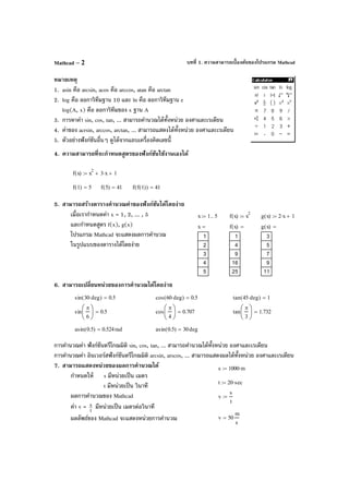
![บทที่ 1. ความสามารถเบื้องต้นของโปรแกรม Mathcad Mathcaad – 3
8. ความสามารถในการเขียนกราฟได้หลายแบบ
8.1 กราฟในระบบพิกัดมุมฉาก
ตัวอย่าง กราฟของ f(x) = 2x + 3 บนช่วง [–5, 5]
8.2 สามารถเขียนกราฟได้หลายเส้นพร้อมกัน
ตัวอย่าง กราฟของ f(x) = 2x + 3 กับ g(x) = 2
x – 4 บนช่วง [–5, 5]
8.3 สามารถเขียนกราฟแบบคู่ลําดับ
ตัวอย่าง การเขียนกราฟของข้อมูล
นํ้าหนักและส่วนสูง
นํ้าหนัก ความสูง
53 156
58 165
55 162
60 170
62 165
68 173
x 5− 4.99−, 5..:= f x( ) 2 x⋅ 3+:=
5 4 3 2 1 0 1 2 3 4 5
10
5
5
10
15
20
f x( )
x
x 5− 4.99−, 5..:= f x( ) 2 x⋅ 3+:= g x( ) x
2
4−:=
5 4 3 2 1 0 1 2 3 4 5
10
5
5
10
15
20
f x( )
g x( )
x
ORIGIN 1:= i 1 6..:=
x
53
58
55
60
62
68
:= y
156
165
162
170
165
173
:=
50 55 60 65 70
150
160
170
180
180
150
yi
7050 xi](https://image.slidesharecdn.com/bookmathcadmathemeticamatlapmaple-160531122930/85/Book-mathcad-mathematica-matlap-maple-12-320.jpg)
![บทที่ 1. ความสามารถเบื้องต้นของโปรแกรม Mathcad Mathcaad – 5
8.7 สามารถปรับเปลี่ยนรูปแบบของกราฟให้เหมาะสมกับการใช้งาน
ตัวอย่าง กราฟของ f(x) = 3
x + 2
x – 9x – 9 บนช่วง [–4, 4]
แบบที่ 1. มีแกน X และแกน Y แต่ไม่มีสเกล แบบที่ 2. มีแกน X และแกน Y มีสเกล
แต่ไม่มีตัวเลขที่สเกล
แบบที่ 3. มีแกน X และแกน Y แบบที่ 4. มีแกน X และแกน Y
มีสเกลและมีตัวเลขที่สเกล มีสเกล มีตัวเลขที่สเกล
มีเส้นกริดช่วยในการประมาณค่า
8.8 สามารถเขียนกราฟ 2 ฟังก์ชันที่มีโดเมนต่างกันได้
ตัวอย่าง กราฟของ f(x) = 5 – 4x บนช่วง [–3, 1] และ g(t) = 2t + 10 บนช่วง [1, 4]
x 4− 3.99−, 4..:= f x( ) x
3
x
2
9 x⋅− 9−+:=
0
f x( )
x
x 4− 3.99−, 4..:= f x( ) x
3
x
2
9 x⋅− 9−+:=
f x( )
x
x 4− 3.99−, 4..:= f x( ) x
3
x
2
9 x⋅− 9−+:=
4 3 2 1 0 1 2 3 4
40
20
20
40
f x( )
x
x 3− 2.99−, 1..:= f x( ) 5 4 x⋅−:= t 1 1.01, 4..:= g t( ) 2 t⋅ 10+:=
4 3 2 1 0 1 2 3 4 5
5
5
10
15
20
f x( )
g t( )
x t,
.
x 4− 3.99−, 4..:= f x( ) x
3
x
2
+ 9 x⋅− 9−:=
4 3 2 1 0 1 2 3 4
40
20
20
40
f x( )
x](https://image.slidesharecdn.com/bookmathcadmathemeticamatlapmaple-160531122930/85/Book-mathcad-mathematica-matlap-maple-14-320.jpg)
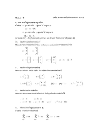
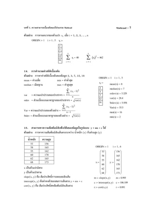
![บทที่ 1. ความสามารถเบื้องต้นของโปรแกรม MathcadMathcad – 8
16. ความสามารถในการจัดรูปพีชคณิต การแยกตัวประกอบ การกระจายพหุนาม
16.1 การกระจายพหุนาม
ตัวอย่าง
16.2 การแยกตัวประกอบ
ตัวอย่าง
16.3 การจัดรูปแบบทางพีชคณิต
ตัวอย่าง
17. ความสามารถในการหาอนุพันธ์ และอนุพันธ์ย่อย ทั้งแบบค่าตัวเลขและเป็ นสูตร
17.1 การหาอนุพันธ์เป็นค่าตัวเลข
ตัวอย่าง การหาอนุพันธ์
ตัวอย่าง การหาอนุพันธ์ย่อย
17.2 การหาอนุพันธ์เป็นสูตร
ตัวอย่าง การหาอนุพันธ์
ตัวอย่าง การหาอนุพันธ์ย่อย
x 1−( ) x 2+( )⋅ expand x
2
x 2−+→
x 1+( ) x 2+( )
2
⋅ expand x
3
5 x
2
⋅+ 8 x⋅+ 4+→
x
2
5 x⋅+ 6+ factor x 3+( ) x 2+( )⋅→
x
3
5 x
2
⋅+ 8 x⋅+ 4+ factor x 1+( ) x 2+( )
2
⋅→
1
2
2
3
+ factor
7
6
→
1
1 2+
factor 2 1−→
1
1 x−
1
1 x+
+ factor
2−
x 1−( ) x 1+( )⋅[ ]
→
x 1:= f x( ) x
3
4 x
2
⋅+ 5 x⋅+ 4−:=
f x( ) 6=
x
f x( )
d
d
16=
2
x
f x( )
d
d
2
14=
3
x
f x( )
d
d
3
6=
x 2:= y 1:=
x
x
3
2 x
2
⋅ y⋅+ y
4
+( )d
d
20=
y y
x
3
2 x
2
⋅ y⋅+ y
4
+( )d
d
d
d
12=
x
x
3
4 x
2
⋅+ 5 x⋅+ 4−( )d
d
expand 3 x
2
⋅ 8 x⋅+ 5+→
2
x
x
3
4 x
2
⋅+ 5 x⋅+ 4−( )d
d
2
expand 6 x⋅ 8+→
x
x
3
2 x
2
⋅ y⋅+ y
4
+( )d
d
simplify 3 x
2
⋅ 4 x⋅ y⋅+→
y y
x
3
2 x
2
⋅ y⋅+ y
4
+( )d
d
d
d
simplify 12 y
2
⋅→](https://image.slidesharecdn.com/bookmathcadmathemeticamatlapmaple-160531122930/85/Book-mathcad-mathematica-matlap-maple-17-320.jpg)
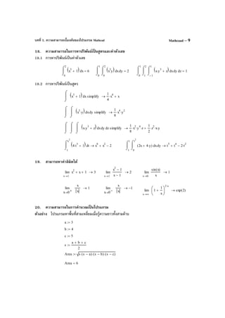
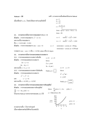
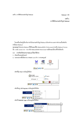
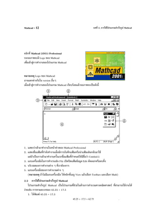
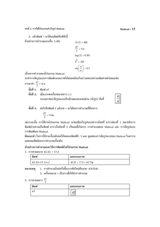
![บทที่ 2. การใช้โปรแกรมสําเร็จรูป Mathcad Mathcad - 17
&
หมายเหตุ กด & จะได้เครื่องหมายปริพันธ์
f(x)<Tab>
หมายเหตุ การกด Tab จะทําให้ curser เลื่อน
ตําแหน่งไปตําแหน่งถัดไป
x<Tab>
1<Tab>
4=↵
1
4
xf x( )
⌠
⌡
d 33=
2.3 การเขียนกราฟของฟังก์ชัน ตัวอย่าง การเขียนกราฟของ f(x) = 2
x - 3x - 7 บนช่วง [-8, 8]
พิมพ์ ผลบนจอภาพ
กําหนดสูตรของ f(x) โดยพิมพ์
f(x):x^2
<Space bar>
-3*x-7↵ f x( ) x
2
3 x⋅− 7−:= .
กําหนดช่วงของ x โดยพิมพ์
x:-8
,
หมายเหตุ กด , เพื่อบอกค่าถัดไปของ x
-7.9
หมายเหตุ x เพิ่มค่าครั้งละ 0.1
;
หมายเหตุ กด ; จะได้สัญลักษณ์ ..
8↵ x 8− 7.9−, 8..:= .
หมายเหตุ x มีค่าจาก -8 ถึง 8 โดยเพิ่มค่าครั้งละ 0.1](https://image.slidesharecdn.com/bookmathcadmathemeticamatlapmaple-160531122930/85/Book-mathcad-mathematica-matlap-maple-26-320.jpg)
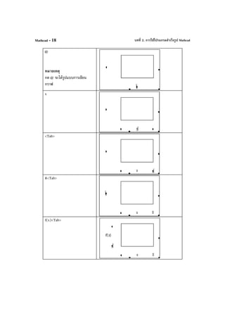
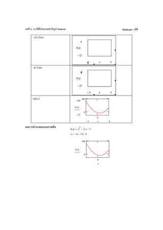
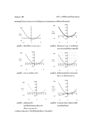
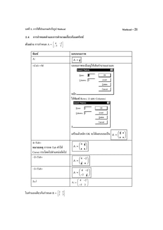
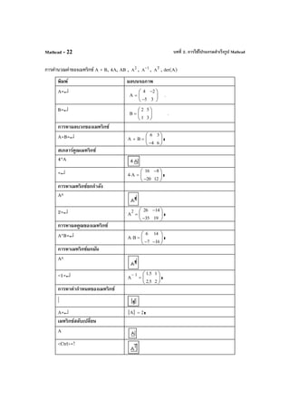
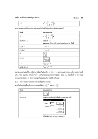
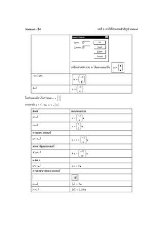
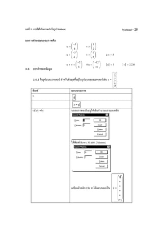
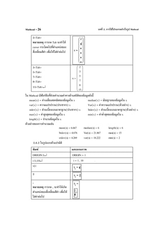
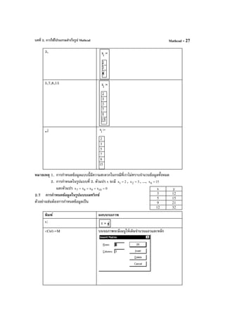
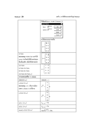
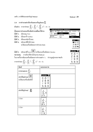
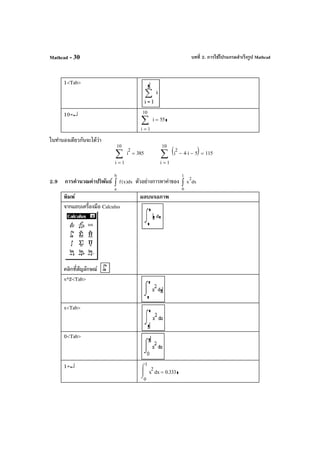
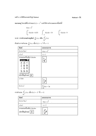
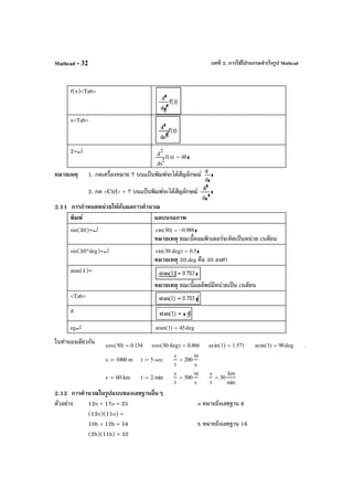
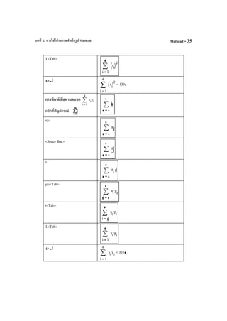
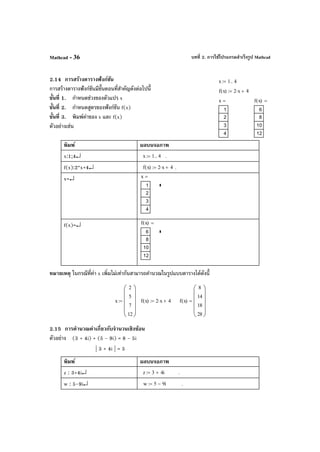
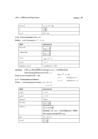
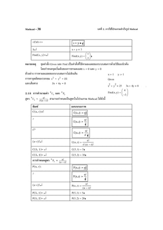
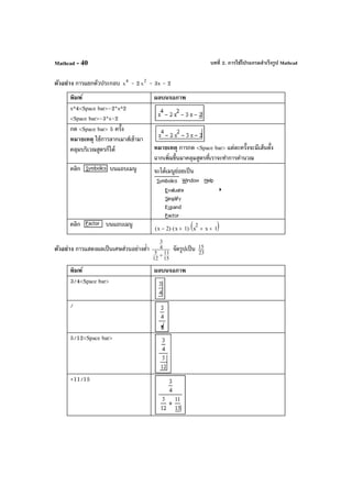
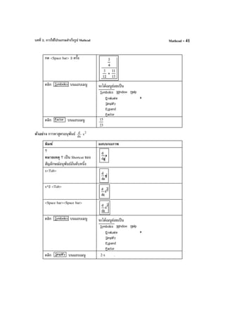
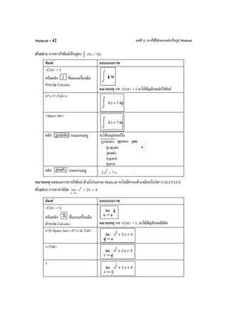
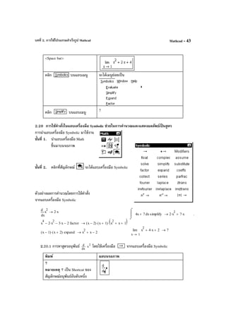
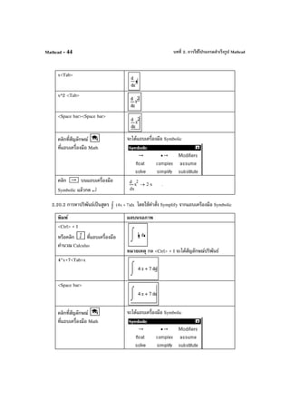
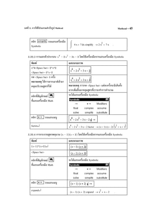
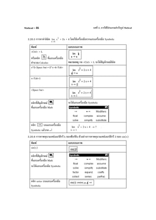
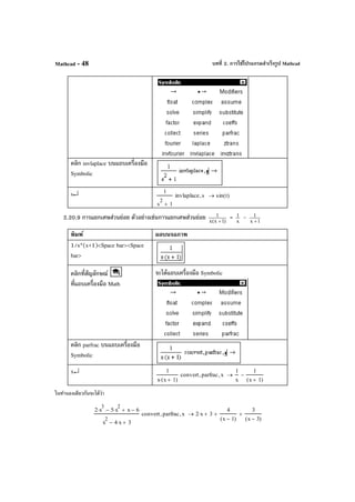
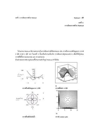
![บทที่ 3. การเขียนกราฟด้วย MathcadMathcad – 50
3.1 การเขียนกราฟในพิกัด XY และการปรับรูปแบบของกราฟ
ตัวอย่าง การเขียนกราฟของ f(x) = 2x + 3 บนช่วง [0, 10]
พิมพ์ ผลบนจอภาพ
f(x):2*x+3↵ f x( ) 2 x⋅ 3+:=
x:0,0.1;10 x 0 0.1, 10..:= .
คลิก ที่แถบเครื่องมือ
จะได้แถบเครื่องมือ Graph
คลิก
บนแถบเครื่องมือ Graph
หมายเหตุ กดเครื่องหมาย @
จะได้สัญลักษณ์ของการเขียน
กราฟ X-Y เหมือนกัน
x<Tab>
10<Tab>
หมายเหตุ 1. การกําหนด x:=0,0.1..10 แปลว่าค่า x มีค่าเป็น 0, 0.1, 0.2, ... , 10
เพราะฉะนั้นมีการเขียนกราฟทั้งหมด 101 จุด
2. ในกรณีที่พิมพ์เฉพาะ x และ f(x) โปรแกรม Mathcad ก็สามารถเขียนกราฟได้](https://image.slidesharecdn.com/bookmathcadmathemeticamatlapmaple-160531122930/85/Book-mathcad-mathematica-matlap-maple-59-320.jpg)
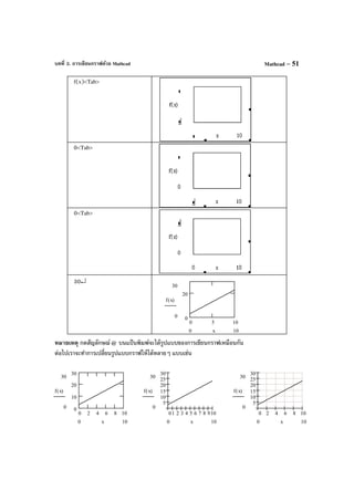
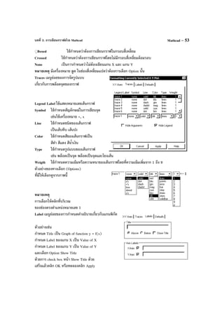
![บทที่ 3. การเขียนกราฟด้วย MathcadMathcad – 54
ภาพที่ได้คือ
Defaults เมนูย่อยกําหนดค่ามาตรฐานของการเขียนกราฟ
ใช้ในการเลือกการ
การกําหนดลักษณะกราฟ (Format)
ตามที่โปรแกรม Mathcad กําหนดไว้
ตัวอย่างการเปลี่ยนรูปแบบ การเขียนกราฟของ f(x) = 2x + 3 บนช่วง [0, 10]
จากรูปเดิม ให้กลายเป็น
ขั้นที่ 1. นําเมาส์ไปกดดับเบิลคลิกที่บริเวณ
ของกราฟจะได้เมนูของการ Format กราฟ
ขั้นที่ 2.
กําหนดทางเลือก (Options) ใน X-Y Axes ดังนี้
1. คลิกที่ Auto Grid ของ แกน X
ให้เครื่องหมายถูก หายไปเพื่อยกเลิก Auto Grid
2. พิมพ์ 5 ในช่อง No. of Grids ของ แกน X
3. คลิกที่ Auto Grid ของ แกน Y
ให้เครื่องหมายถูก หายไปเพื่อยกเลิก Auto Grid
4. พิมพ์ 3 ในช่อง No. of Grids ของ แกน Y
ขั้นที่ 3. คลิก OK หรือ คลิก Apply ภาพที่ได้คือ
0 2 4 6 8 10
0
10
20
30
30
0
f x( )
100 x
0 2 4 6 8 10
0
10
20
30
30
0
f x( )
100 x
0 5 10
0
20
30
0
f x( )
100 x
0 5 10
0
20
Graph of function y = f(x)
Value of x
Valueofy
30
0
f x( )
100 x](https://image.slidesharecdn.com/bookmathcadmathemeticamatlapmaple-160531122930/85/Book-mathcad-mathematica-matlap-maple-63-320.jpg)
![บทที่ 3. การเขียนกราฟด้วย Mathcad Mathcad – 55
ตัวอย่างการเปลี่ยนรูปแบบ การเขียนกราฟของ f(x) = 2x + 3 บนช่วง [0, 10]
จากรูปเดิม ให้กลายเป็น
ขั้นที่ 1. นําเมาส์ไปกดดับเบิลคลิกที่บริเวณของกราฟจะได้เมนูของการ Format กราฟ
ขั้นที่ 2.
กําหนดทางเลือก (Options) ใน X-Y Axes ดังนี้
1. คลิกที่ Auto Grid ของ แกน X
ให้เครื่องหมายถูกหายไป
เพื่อยกเลิก Auto Grid
2. พิมพ์ 10 ในช่อง No. of Grids ของ แกน X
3. คลิกที่ Auto Grid ของ แกน Y
ให้เครื่องหมายถูก หายไป
เพื่อยกเลิก Auto Grid
4. พิมพ์ 6 ในช่อง No. of Grids ของ แกน Y
5. คลิกที่วงกลมหน้า Crossed
ให้เกิดจุดดําในวงกลม
6. เสร็จแล้วคลิก OK หรือ คลิก Apply
จะได้ภาพตามที่ต้องการ
ตัวอย่างการเปลี่ยนรูปแบบ การเขียนกราฟของ f(x) = 2x + 3 บนช่วง [0, 10]
จากรูปเดิม ให้กลายเป็น
01 2 3 4 5 6 7 8 910
5
10
15
20
25
30
30
0
f x( )
100 x
0 2 4 6 8 10
0
10
20
30
30
0
f x( )
100 x
01 2 3 4 5 6 7 8 910
5
10
15
20
25
30
30
0
f x( )
100 x
0 2 4 6 8 10
5
10
15
20
25
30
30
0
f x( )
100 x](https://image.slidesharecdn.com/bookmathcadmathemeticamatlapmaple-160531122930/85/Book-mathcad-mathematica-matlap-maple-64-320.jpg)
![บทที่ 3. การเขียนกราฟด้วย MathcadMathcad – 56
ขั้นที่ 1. นําเมาส์ไปกดดับเบิลคลิกที่บริเวณของกราฟจะได้เมนูของการ Format กราฟ
ขั้นที่ 2.
กําหนดทางเลือก (Options) ใน X-Y Axes ดังนี้
1. คลิกที่ Auto Grid ของ แกน X
ให้เครื่องหมายถูกหายไป
เพื่อยกเลิก Auto Grid
2. พิมพ์ 10 ในช่อง No. of Grids ของ แกน X
3. คลิกที่ Auto Grid ของแกน Y
ให้เครื่องหมายถูกหายไป
เพื่อยกเลิก Auto Grid
4. พิมพ์ 6 ในช่อง No. of Grids ของ แกน Y
5. คลิกที่ช่อง Grid Line ให้เกิดเครื่องหมายถูก
ทั้งของแกน X และแกน Y
6. เสร็จแล้วคลิก OK หรือ คลิก Apply
จะได้ภาพตามที่ต้องการ
3.2 การย่อและขยายขนาดของกราฟ
เขียนกราฟ f(x) = 2x + 3 บนช่วง [0, 10]
เพื่อเป็นตัวอย่างในการย่อและขยาย
ขั้นตอนการย่อและขยายขนาดกราฟ
ขั้นที่ 1. ลากเมาส์เข้าไปคลุมบริเวณของกราฟ จะเกิดกรอบสี่เหลี่ยมที่มีเส้นแบบเส้นไข่ปลาล้อมรอบกราฟ](https://image.slidesharecdn.com/bookmathcadmathemeticamatlapmaple-160531122930/85/Book-mathcad-mathematica-matlap-maple-65-320.jpg)
![บทที่ 3. การเขียนกราฟด้วย Mathcad Mathcad – 57
ขั้นที่ 2. ขณะที่กรอบเส้นไข่ปลาล้อมรอบกราฟ ให้ปล่อยมือจะเกิดสี่เหลี่ยมขอบเส้นตรงคลุมกราฟ
ขั้นที่ 3. ลากเมาส์ไปยังจุดสีดําที่ขอบของกรอบสี่เหลี่ยมจะเกิด
สัญลักษณ์ ↔ หรือ หรือ การย่อหรือขยายทําได้โดยลาก
เมาส์ ขณะที่เกิดลูกศรตรงขอบทีเอาเมาส์ไปเลือกไว้
1. ย่อหรือขยายทางด้านข้าง
2. ย่อหรือขยายทางด้านบน และ ล่าง
3. ย่อหรือขยายทั้งสองด้านพร้อมกัน
ตัวอย่างการย่อหรือขยายเช่น
3.3 การ COPY CUT และ PASTE กราฟ
เขียนกราฟของ f(x) = 2x + 3
บนช่วง [0, 10] เพื่อเป็นตัวอย่าง
นําเมาส์เข้าไปคลิกที่บริเวณของกราฟ
จะได้สี่เหลี่ยมที่มีเส้นทึบคลุมรูป
กดฟังก์ชันคีย์ F2 หรือ <Ctrl> + C
เป็นการ Copy กราฟรูปนี้
เลื่อน Curser ไปที่บริเวณนอกกราฟรูปเดิม
0 1 2 3 4 5 6 7 8 9 10
0
5
10
15
20
25
30
30
0
f x( )
100 x
01 23 45 6 78 910
0
5
10
15
20
25
30
30
0
f x( )
100 x
0 1 2 3 4 5 6 7 8 9 10
0
5
10
15
20
25
30
30
0
f x( )
100 x](https://image.slidesharecdn.com/bookmathcadmathemeticamatlapmaple-160531122930/85/Book-mathcad-mathematica-matlap-maple-66-320.jpg)
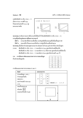
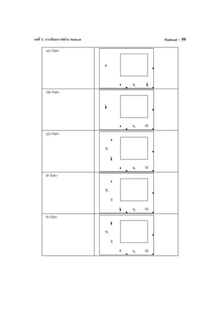
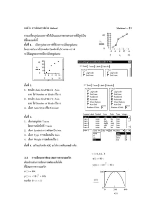
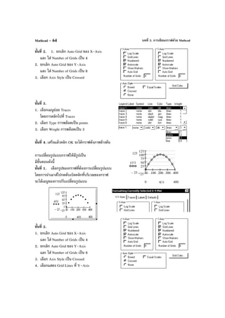
![บทที่ 3. การเขียนกราฟด้วย Mathcad Mathcad – 65
ขั้นที่ 3. 1. เลือกเมนูย่อย Traces
โดยการคลิกไปที่ Traces
2. เลือก Symbol การพล็อตเป็น box
3. เลือก Type การพล็อตเป็น points
4. เลือก Weight การพล็อตเป็น 1
ขั้นที่ 4. เสร็จแล้วคลิก OK จะได้กราฟดังภาพข้างต้น
3.6 การเขียนกราฟของสมการในพิกัดเชิงขั้ว
ตัวอย่างเช่นการเขียนกราฟของฟังก์ชัน
r(t) = 5sin(2t) บนช่วง ]2,0[ π
วิธีทํา
ขั้นตอนการเขียนกราฟพิกัดเชิงขั้ว
พิมพ์ ผลบนจอภาพ
t:0,0.1;2*π↵
r(t):5*sin(2*t)
t 0 0.1, 2 π⋅..:=
r t( ) 5 sin 2 t⋅( )⋅:=
คลิก ที่แถบเครื่องมือ
จะได้แถบเครื่องมือ Graph
คลิก
บนแถบเครื่องมือ Graph
หมายเหตุ <Ctrl> + 7
จะได้สัญลักษณ์ของการเขียน
กราฟพิกัดเชิงขั้ว
t<Tab>
t 0 0.1, 2 π⋅..:=
r t( ) 5 sin 2 t⋅( )⋅:=
0
30
60
90
120
150
180
210
240
270
300
330
4
2
0
5
0r t( )
t](https://image.slidesharecdn.com/bookmathcadmathemeticamatlapmaple-160531122930/85/Book-mathcad-mathematica-matlap-maple-74-320.jpg)
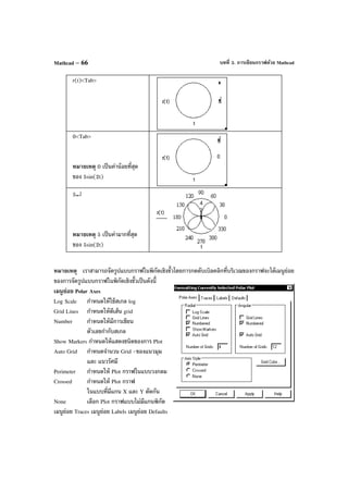
![บทที่ 3. การเขียนกราฟด้วย Mathcad Mathcad – 67
มีหน้าที่เหมือนกราฟในพิกัดแกน XY (ดูหัวข้อ 3.1) ตัวอย่างการจัดรูปแบบของกราฟและภาพของกราฟที่ได้
3.7 การเขียนกราฟแบบ 3 มิติ
ตัวอย่างเช่น กราฟของ f(x, y) = 2
x – 2
y บนช่วง [–2, 2] × [–2, 2]
การเขียนกราฟพื้นผิว 3 มิติ แบบที่ 1.
พิมพ์ ผลบนจอภาพ
x:-2,-1.99;2↵ x 2− 1.99−, 2..:= .
y:-2;-1.99;2↵ y 2− 1.99−, 2..:= .
f(x,y):x^2<Space bar>–y^2↵ f x y,( ) x
2
y
2
−:= .
คลิก
บนแถบเครื่องมือ Graph
หมายเหตุ <Ctrl> + 2
จะได้สัญลักษณ์ของการเขียนกราฟ
3 มิติ
f↵
f
.
0
45
90
135
180
225
270
315
543210
5
0r t( )
t](https://image.slidesharecdn.com/bookmathcadmathemeticamatlapmaple-160531122930/85/Book-mathcad-mathematica-matlap-maple-76-320.jpg)
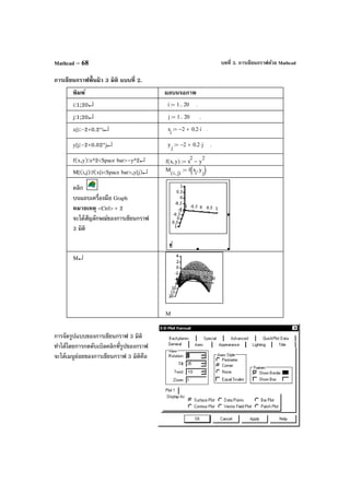
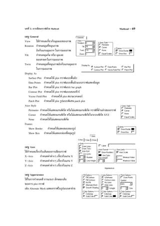
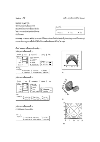
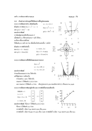
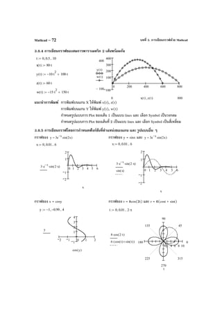
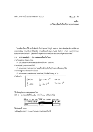
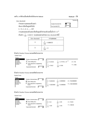
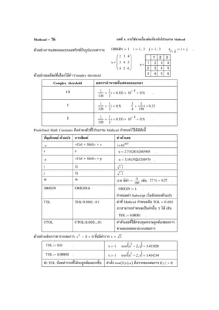
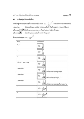
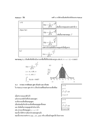
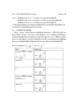
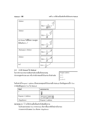
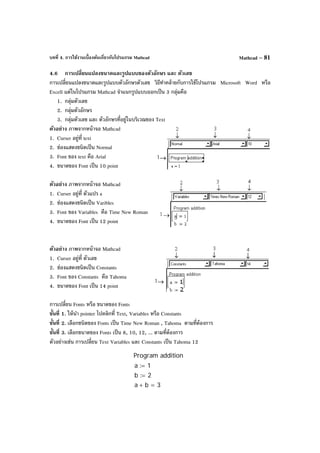
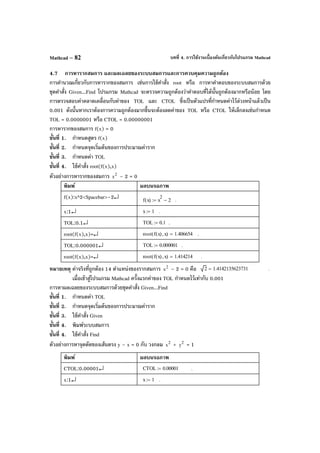
![บทที่ 4. การใช้งานเบื้องต้นเกี่ยวกับโปรแกรม Mathcad Mathcad – 83
y:1↵ y 1:= .
Given↵ Given .
y-x<Ctrl>+=0↵ x y− 0 .
x^2<Spacebar>–+y^2
<Spacebar><Ctrl>+=1↵
x
2
y
2
+ 1 .
Find(x,y)=↵
y
Find x y,( )
0.7071054437
0.7071054437
= .
หมายเหตุ เมื่อเราลดขนาดของ CTOL ผลการคํานวณจะถูกต้องมากขึ้น ตัวอย่างเช่น
หมายเหตุ พิกัดจุดตัดที่แท้จริงคือ (x = 0.707106781186547 , y = 0.707106781186547)
4.8 การบันทึกแฟ้ มข้อมูล Mathcad และ เรียกแฟ้ มข้อมูลขึ้นมาทํางาน
เมื่อเริ่มทํางานครั้งแรกกับ Mathcad จะเห็นว่าชื่อแฟ้ มของงานที่เราทําจะมีชื่อที่โปรแกรม Mathcad กําหนดคือ
[Untitled: 1] สมมติงานที่เราทําขณะนี้คือ โปรแกรมการหารากสมการ
4.8.1 การบันทึกแฟ้ มข้อมูล
ขั้นที่ 1. คลิกที่ File และเลือก คําสั่ง Save
จะได้เมนูย่อยของการบันทึกแฟ้ ม
ขั้นที่ 2. พิมพ์ชื่อแฟ้ มตามที่ต้องการเช่น Findroot
CTOL 0.00001:=
x 1:=
y 1:=
Given
x y− 0
x
2
y
2
+ 1
Find x y,( )
0.707105443654304
0.707105443654304
= .
CTOL 0.0000001:=
x 1:=
y 1:=
Given
x y− 0
x
2
y
2
+ 1
Find x y,( )
0.707106776742374
0.707106776742374
= .](https://image.slidesharecdn.com/bookmathcadmathemeticamatlapmaple-160531122930/85/Book-mathcad-mathematica-matlap-maple-92-320.jpg)
![บทที่ 4. การใช้งานเบื้องต้นเกี่ยวกับโปรแกรม MathcadMathcad – 84
ขั้นที่ 4. คลิกที่ Save
จะเห็นว่า [Untitled: 1] กลายเป็น [Findroot] แล้ว
4.8.1 การเรียกแฟ้ มข้อมูลเก่าขึ้นมาทํางาน
สมมติขณะนี้จอภาพของเราว่าง
เนื่องจากเข้ามาสู่ Mathcad ครั้งแรก
ขั้นที่ 1. คลิกที่ File และเลือกคําสั่ง Open
จะได้เมนูย่อยของการเปิดแฟ้ ม
ขั้นที่ 2. พิมพ์ชื่อแฟ้ มที่ต้องการเปิดคือ Findroot
ขั้นที่ 3. คลิก Open จะได้แฟ้ มข้อมูลที่ต้องการ
หมายเหตุ คําสั่ง FileNew.. คําสั่ง FileSave As.. คําสั่ง FileClose.. มีลักษณะใช้งานเหมือนกับการทํางาน
ทั่วไปของระบบ Windows](https://image.slidesharecdn.com/bookmathcadmathemeticamatlapmaple-160531122930/85/Book-mathcad-mathematica-matlap-maple-93-320.jpg)
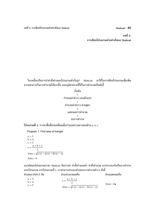
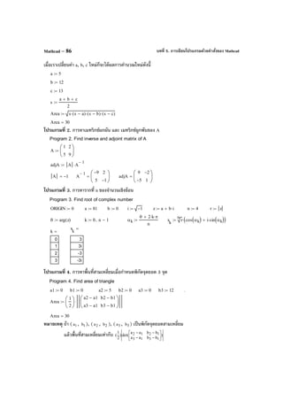
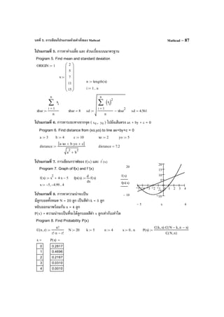
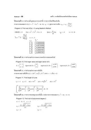
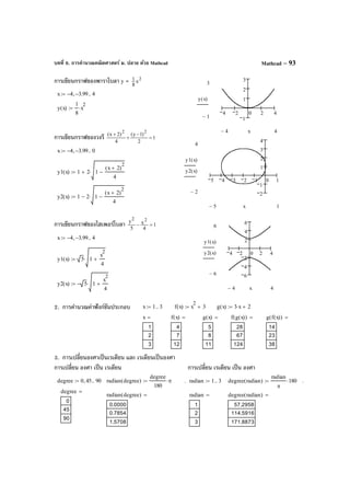
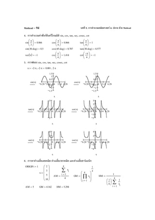
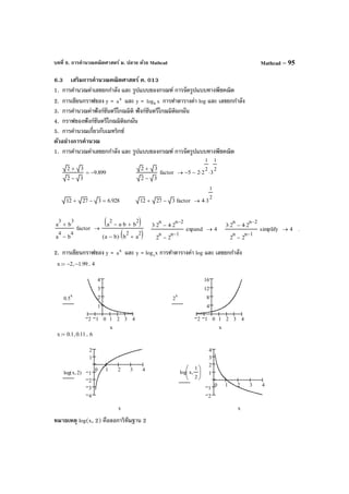
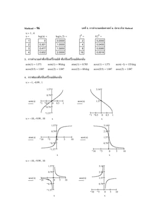
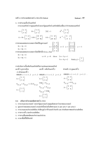
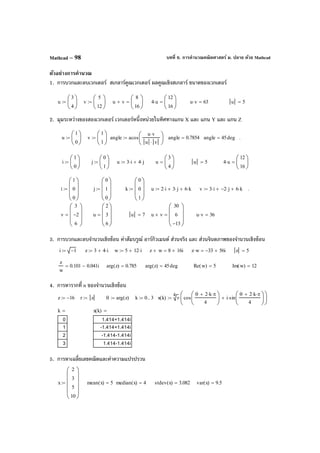
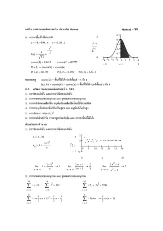
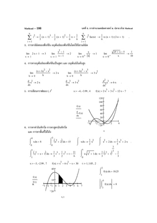
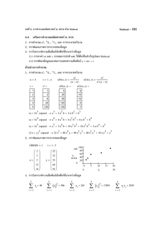
![บทที่ 6. การคํานวณคณิตศาสตร์ ม. ปลาย ด้วย MathcadMathcad – 102
3.1 การหาค่า m และ c จากสมการปกติ
การหาค่า m และ c โดยใช้ฟังก์ชันสําเร็จรูปของ Mathcad
3.2 กราฟของข้อมูลและสมการแสดงความสัมพันธ์ y = mx + c
6.7 Mathcad กับการเฉลยข้อสอบคณิตศาสตร์ Entrance
ในหัวข้อนี้จะเป็นการนําความสามารถของ Mathcad เข้ามาช่วยหาคําตอบของข้อสอบ Entrance ซึ่งมีข้อสอบ
Entrance เป็นจํานวนมากที่เราอาจจะหาคําตอบได้ด้วยการแทนค่า คํานวณค่า หรือแม้แต่เขียนกราฟดูก็จะได้
คําตอบ
ข้อสอบคณิตศาสตร์ 1. มีนาคม 2546 ข้อ 18.
0x
lim
→ 3
x
1 [ x1+ – x1− – )x1)(x1( 2
−+ + )x1)(x1( 2
−− ] มีค่าเท่ากับข้อใดต่อไปนี้
1. 0 2. 4
1
3. 2
1 4. 1
การคํานวณด้วย Mathcad
เพราะฉะนั้นตอบข้อ 3.
m 0:= c 0:= Given 5 c⋅ 40 m⋅+ 265
40 c⋅ 506 m⋅+ 2839
Find m c,( )
3.866
22.075
=
m slope x y,( ):= m 3.866=
c intercept x y,( ):= c 22.075=
t 0 0.1, 20..:= ycap t( ) m t⋅ c+:=
0 5 10 15 20
20
40
60
80
100
yi
ycap t( )
xi t,
0x
1
x
3
1 x+ 1 x−− 1 x+( ) 1 x
2
−( )⋅− 1 x−( ) 1 x
2
−( )⋅+
⋅lim
→
1
2
→](https://image.slidesharecdn.com/bookmathcadmathemeticamatlapmaple-160531122930/85/Book-mathcad-mathematica-matlap-maple-111-320.jpg)
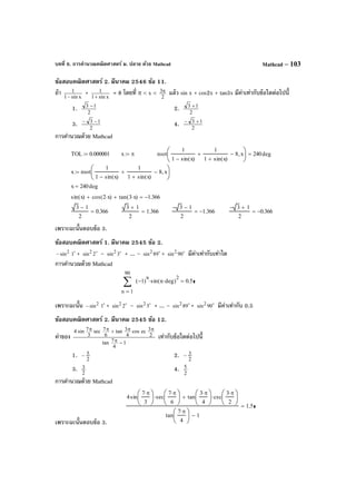
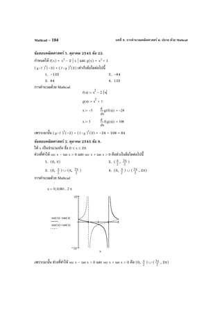
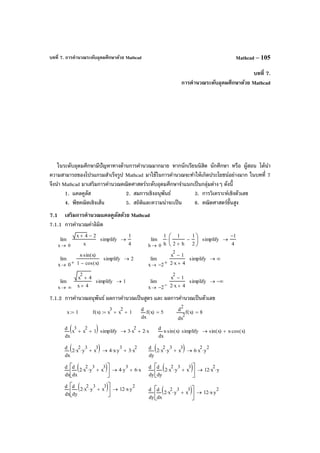
![บทที่ 7. การคํานวณระดับอุดมศึกษาด้วย MathcadMathcad – 106
7.1.3 การคํานวณปริพันธ์ ผลการคํานวณเป็นสูตร และ ผลการคํานวณเป็นตัวเลข
7.1.4 กราฟของฟังก์ชัน f, f′ และ f′′
7.1.5 การหาผลบวกรีมันน์ (Riemann sum) เช่นผลบวกรีมันน์ของ f(x) = 2
x – 4x + 6 บนช่วง [1, 3]
7.1.6 การแทนฟังก์ชันด้วยพหุนามเทย์เลอร์
อนุกรมเทย์เลอร์ของฟังก์ชัน sin(x)
x 4− 3.999−, 4..:= f x( ) x
3
x
2
− 4 x⋅− 4+:=
4 3 2 1 0 1 2 3 4
30
20
10
10
20
30
40
f x( )
x
f x( )
d
d
x
4 3 2 1 0 1 2 3 4
30
20
10
10
20
30
40
f x( )
x
f x( )
d
d
2
x
f x( )
d
d
2
x
sin x( ) series x, 5, 1 x⋅
1
6
x
3
⋅−→ sin x( ) series x, 6, 1 x⋅
1
6
x
3
⋅−
1
120
x
5
⋅+→
f x( ) x
2
4 x⋅− 6+:= n 10:=
a 1:= b 3:= i 1 n..:=
h
b a−
n
:= x
0
a:= x
i
x
i 1−
h+:=
S
1
n
i
f x
i( ) x
i
x
i 1−
−( )⋅∑
=
:=
S 4.68=
f x( ) x
2
4 x⋅− 6+:= n 100:=
a 1:= b 3:= i 1 n..:=
h
b a−
n
:= x
0
a:= x
i
x
i 1−
h+:=
S
1
n
i
f x
i( ) x
i
x
i 1−
−( )⋅∑
=
:=
S 4.6668=
0
3
xx
2⌠
⌡
d 9=
0
π
xsin x( )
⌠
⌡
d 2=
1
t
xx
2⌠
⌡
d
1
3
t
3
⋅
1
3
−→
xx
2
⌠
⌡
d simplify
1
3
x
3
⋅→ xsin x( )
⌠
⌡
d simplify cos x( )−→ xln x( )
⌠
⌡
d x ln x( )⋅ x−→ .
yxx
2
y⋅
⌠
⌡
d
⌠
⌡
d
1
6
x
3
⋅ y
2
⋅→
0
t
y
0
s
xx
2
y⋅
⌠
⌡
d
⌠
⌡
d
1
6
t
2
⋅ s
3
⋅→
0
3
y
0
2
xx
2
y
⌠
⌡
d
⌠
⌡
d 12=
a
b
xf x( )
⌠
⌡
d 4.667= .](https://image.slidesharecdn.com/bookmathcadmathemeticamatlapmaple-160531122930/85/Book-mathcad-mathematica-matlap-maple-115-320.jpg)
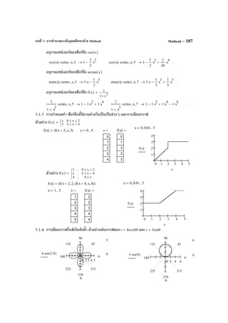
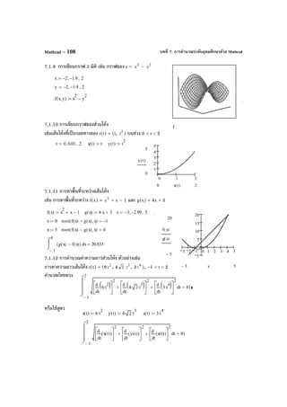
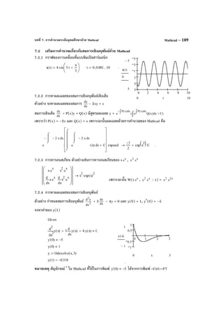
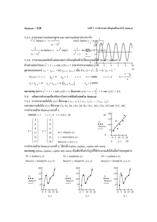
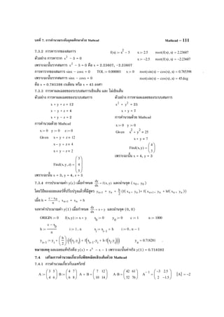
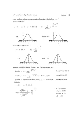
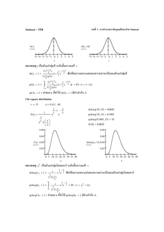
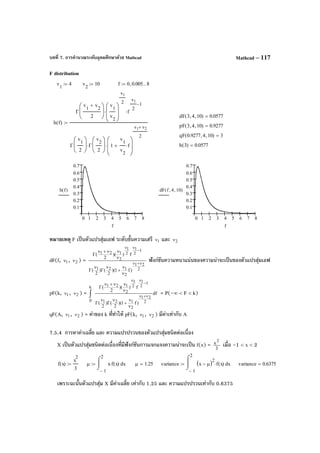
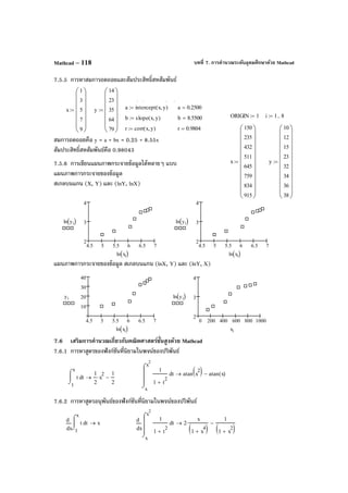
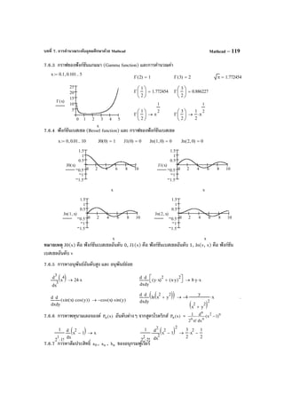

![บทนํา
Mathematica
โปรแกรมสําเร็จรูป Mathematica เป็นโปรแกรมที่มีชื่อเสียงมากและเป็นโปรแกรมที่มีความสามารถใน
การคํานวณสูง รูปแบบการใช้งานต้องพิมพ์คําสั่งผ่านบรรทัดที่เรียกว่า line in [..] ผลของการคํานวณที่ได้จะ
แสดงออกมาที่บรรทัด line out [..] การใช้งานโดยทั่วไปผู้ใช้ต้องจดจําคําสั่งที่ต้องการได้ หรือจะให้
โปรแกรมแสดงแถบเครื่องมือของคําสั่งให้ปรากฏบนจอภาพตลอดเวลาก็ได้ ในการใช้งานโปรแกรม
Mathematica ความสามารถในการทํางานบางอย่าง เช่นงานทางด้าน Graphics จะจําแนกเป็นโปรแกรมย่อย
เรียกว่า Package ซึ่งเราต้องเรียกโปรแกรมย่อยนั้นขึ้นมาก่อนจึงจะใช้งานทางด้าน Graphics ได้
ในการใช้ Package เช่นการเรียก Package Graphics ต้องพิมพ์ <<Graphics `Graphics` จึงจะใช้คําสั่ง
ในกลุ่มของการเขียนกราฟได้ แต่ในการใช้งานจริงเนื่องจากแป้ นพิมพ์บางแป้นพิมพ์ไม่สามารถพิมพ์สัญลักษณ์
backquote character (`) จึงขอแนะนําวิธีพิมพ์คําสั่งเรียกใช้ Package ดังนี้
วิธีที่ 1. พิมพ์ $Packages แล้วกด <Shift>+↵
ผลบนจอภาพจะได้สัญลักษณ์ backquote character (`) ที่ Out[1] ให้เลื่อนเมาส์ไป copy สัญลักษณ์
backquote character (`) ที่ได้ไว้ใช้งานต่อไปเมื่อต้องการพิมพ์ backquote character (`)
วิธีที่ 2. คลิกที่ Help เมื่อได้เมนูของ Help แล้วให้เลือก Add–on Standard Package Graphics
Graphics จะได้คําอธิบายต่าง ๆ ของการใช้ Package Graphics ให้ทําการ copy คําว่า Graphics`Graphics` มา
paste ที่บรรทัด line in เพื่อใช้ในการเรียก Package Graphics ต่อไป
ความสามารถที่เหมือนและแตกต่างจาก Mathcad เช่น
• Mathematica แสดงผลทศนิยมได้หลายตําแหน่งตามต้องการแต่ Mathcad แสดงผลได้สูงสุด 15 ตําแหน่ง
• การปรับเปลี่ยนรูปแบบการแสดงผลของกราฟ ต้องใช้คําสั่งในการกําหนดค่า ไม่เหมือนกับ Mathcad ที่มี
เมนูของการปรับเปลี่ยนรูปแบบกราฟ
• มีแถบเครื่องมือในการคํานวณ สามารถนําแถบเครื่องมือมาแสดงบนจอภาพได้เหมือนกัน
• สามารถขอคําอธิบายของคําสั่ง ด้วยการพิมพ์ ? ตามด้วยคําสั่งที่ต้องการรู้ความหมาย แล้วกด Enter
สารบัญ
บทที่ 1. ความสามารถเบื้องต้นของโปรแกรม Mathematica......................................... 1 – 10
บทที่ 2. การใช้โปรแกรมสําเร็จรูป Mathematica....................................................... 11 – 34
บทที่ 3. การเขียนกราฟด้วย Mathematica............................................................... 35 – 50
บทที่ 4. การใช้งานเบื้องต้นเกี่ยวกับโปรแกรม Mathematica........................................ 51 – 62
บทที่ 5. การเขียนโปรแกรมด้วยคําสั่งของ Mathematica............................................. 63 – 68
บทที่ 6. การคํานวณคณิตศาสตร์ ม. ปลาย ด้วย Mathematica..................................... 69 – 78
บทที่ 7. การคํานวณระดับอุดมศึกษาด้วย Mathematica.............................................. 79 – 94](https://image.slidesharecdn.com/bookmathcadmathemeticamatlapmaple-160531122930/85/Book-mathcad-mathematica-matlap-maple-131-320.jpg)
![บทที่ 1. ความสามารถเบื้องต้นของโปรแกรม Mathematica Mathematica - 1
บทที่ 1.
ความสามารถเบื้องต้นของโปรแกรม Mathematica
ในบทนี้เป็นการนําความสามารถเบื้องต้นของโปรแกรมสําเร็จรูป Mathematica ทําได้มาให้ดูก่อนเพื่อผู้อ่าน
จะได้เห็นความสามารถทางการคํานวณที่สําคัญของโปรแกรมสําเร็จรูป Mathematica ในส่วนของการพิมพ์
คําสั่ง การเข้าสู่โปรแกรม Mathmatica และการประยุกต์ต่าง ๆ จะกล่าวในบทต่อไป
เนื่องจากลักษณะการทํางานของโปรแกรม Mathematica มีบรรทัดของคําสั่งที่เราต้องพิมพ์คําสั่งของการ
คํานวณเข้าไป เรียกว่า line In ln[n] := ... โปรแกรม Mathematica จึงจะแสดงผลการคํานวณ ในบรรทัดถัดไป
เรียกว่า line out Out[n] = ... ดังนั้น การยกตัวอย่างความสามารถต่าง ๆ จึงขอนําผลการคํานวณที่ปรากฎบน
จอภาพ ซึ่งมีทั้งบรรทัด line in (In[n] :=) และ line out (Out[n]=)
1. การคํานวณเบื้องต้น บวก ลบ คูณ หาร และเลขยกกําลัง
2. สามารถกําหนดการแสดงผลการคํานวณให้เป็ นทศนิยมได้หลายตําแหน่ง
แสดงค่าของ π เป็นเลขทศนินม 5 ตําแหน่ง แสดงค่าของ π เป็นเลขทศนิยม 20 ตําแหน่ง
3. มีฟังก์ชันทางคณิตศาสตร์ให้ใช้มากมาย](https://image.slidesharecdn.com/bookmathcadmathemeticamatlapmaple-160531122930/85/Book-mathcad-mathematica-matlap-maple-132-320.jpg)
![บทที่ 1. ความสามารถเบื้องต้นของโปรแกรม MathematicaMathematica - 2
หมายเหตุ E หมายถึง ค่า e มีค่าประมาณเท่ากับ 2.71828
Log[a, x] หมายถึง log ฐาน a ของ x
Log[x] หมายถึง log ฐาน e ของ x
4. มีความสามารถในการกําหนดฟังก์ชันใช้งานได้
หมายเหตุ f[x_] คือ การกําหนดสูตรของฟังก์ชัน f(x)
5. สามารถกําหนดเซตของจํานวน และสามารถคํานวณสมาชิกภายในเซตได้
หมายเหตุ เซตของตัวเลขเป็นชนิดของตัวแปรแบบหนึ่งใน Mathematica ซึ่งเรียกว่าตัวแปรแบบ list
6. สามารถเปลี่ยนหน่วยการคํานวณได้โดยง่าย
หมายเหตุ ถ้าไม่กําหนดหน่วยของมุมฟังก์ชันตรีโกณมิติใน Mathematica จะคิดหน่วยของมุมเป็นเรเดียน
การระบุหน่วยให้พิมพ์ Degree ต่อท้ายตัวเลข
การเติมจุดท้ายตัวเลขจะทําให้ผลการคํานวณแสดงค่าเป็นเลขทศนิยม
7. ความสามารถในการแสดงหน่วยของผลการคํานวณ](https://image.slidesharecdn.com/bookmathcadmathemeticamatlapmaple-160531122930/85/Book-mathcad-mathematica-matlap-maple-133-320.jpg)
![บทที่ 1. ความสามารถเบื้องต้นของโปรแกรม Mathematica Mathematica - 5
9. การคํานวณในรูปแบบเลขฐานต่าง ๆ
2^^10101 หมายถึงจํานวน 10101 ฐาน 2
รูปแบบทั่วไป b^^xx...x หมายถึง xx...x ฐาน b
หมายถึงการเปลี่ยน 21 ฐาน 10 เป็นจํานวนใบระบบฐาน 2
รูปแบบทั่วไป BaseForm[N, b]
คือการเปลี่ยนจาก N ฐาน 10 เป็น จํานวนในระบบฐาน b
ตัวอย่างอื่น ๆ เช่น
10. การคํานวณในรูปแบบเวกเตอร์
11. การคํานวณในรูปแบบเมทริกซ์
12. การคํานวณจํานวนเชิงซ้อน
หมายเหตุ การพิมพ์สัญลักษณ์ i ให้พิมพ์ <Ecs>ii<Ecs>](https://image.slidesharecdn.com/bookmathcadmathemeticamatlapmaple-160531122930/85/Book-mathcad-mathematica-matlap-maple-136-320.jpg)
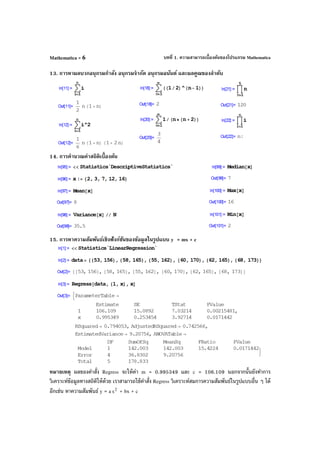
![บทที่ 1. ความสามารถเบื้องต้นของโปรแกรม Mathematica Mathematica - 7
16. ความสามารถในการจัดรูปพีชคณิต การแยกตัวประกอบ การกระจายพหุนาม
17. ความสามารถในการหา อนุพันธ์ อนุพันธ์อันดับสูง อนุพันธ์ย่อย แบบเป็ นสูตร และ เป็ นค่าตัวเลข
การหาอนุพันธ์เป็นสูตรและค่าตัวเลข อนุพันธ์อันดับสูง อนุพันธ์ย่อย
หมายเหตุ D[f[x], x] คือ )x(f
dx
d
และ D[f[x], {x, n}] คือ )x(f
dx
d
n
n
และ ]y,x[fy,x
∂ คืออนุพันธ์ย่อย
18. ความสามารถในการหาปริพันธ์ เป็ นสูตร และ เป็ นค่าตัวเลข](https://image.slidesharecdn.com/bookmathcadmathemeticamatlapmaple-160531122930/85/Book-mathcad-mathematica-matlap-maple-138-320.jpg)
![บทที่ 1. ความสามารถเบื้องต้นของโปรแกรม MathematicaMathematica - 8
19. ความสามารถในการหาค่าลิมิต
หมายเหตุ Limit[f[x] , x→ a] คือ )x(flim
ax→
Limit[f[x] , x→ a, Direction → 1] คือ )x(flim
ax −→
Limit[f[x] , x→ a, Direction → –1] คือ )x(flim
ax +→
20. ความสามารถในการคํานวณเป็ นโปรแกรม
โปรแกรมหาพื้นที่สามเหลี่ยมเมื่อรู้ความยาวทั้งสามด้าน
21. ความสามารถในการหารากของสมการ f(x) = 0
หมายเหตุ FindRoot[f[x]==0, {x, a}] คือการหารากของ f(x) = 0 จุดเริ่มต้นของการประมาณค่าที่ x = a](https://image.slidesharecdn.com/bookmathcadmathemeticamatlapmaple-160531122930/85/Book-mathcad-mathematica-matlap-maple-139-320.jpg)
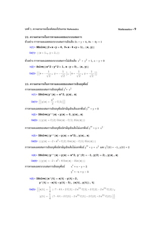
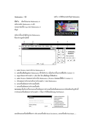
![บทที่ 2. การใช้โปรแกรมสําเร็จรูป Mathematica Mathematica – 13
ตัวอย่างของแถบเครื่องมือเช่น
AlgebraicManipulation BasicCalculations BasicInput
2.2 การใช้โปรแกรมสําเร็จรูป Mathematica
รูปแบบการทํางานด้วยคําสั่งต่าง ๆ ของ Mathematica มีบรรทัดของการรับค่าหรือคําสั่ง และมีบรรทัดของการ
แสดงผล ตัวอย่างเช่น การหาผลบวก 1 + 2 เมื่อเราพิมพ์ 1 + 2 เสร็จแล้วกด <Shift > + ↵ โปรแกรมจะทํา
การคํานวณ แล้วขึ้นบรรทัดใหม่ แล้วแสดงผลการคํานวณให้ ดังนี้
หมายเหตุ กด ↵ เป็นการขึ้นบรรทัดใหม่
การกด <Shift >+↵ (กด Shift ค้างไว้แล้วกด Enter) คือการสั่งให้โปรแกรมทําการคํานวณ
เพื่อให้เข้าใจการใช้งานง่ายขึ้น การใช้งานโปรแกรม Mathematica จะขอเขียนในรูปแบบตาราง โดยมีตาราง
ช่องที่ 1 หมายถึงการพิมพ์ผ่านทางแป้ นพิมพ์ ตารางในช่องที่ 2 เป็นผลที่เกิดจากการคํานวณของ
Mathematica และสิ่งเกิดขึ้นจากผลการคํานวณและการจัดรูปแบบการแสดงผลบนจอภาพที่มี
ln[n] := .....................
และ Out[n]= .....................
การคํานวณด้วยโปรแกรม Mathematica
1. การหาผลบวก 45.25 + 17.5
พิมพ์ ผลบนจอภาพ
45.25+17.5<Shift >+↵](https://image.slidesharecdn.com/bookmathcadmathemeticamatlapmaple-160531122930/85/Book-mathcad-mathematica-matlap-maple-144-320.jpg)
![บทที่ 2. การใช้โปรแกรมสําเร็จรูป MathematicaMathematica – 14
2. การหาผลหาร
5
47
พิมพ์ ผลบนจอภาพ
47/5.<Shift>+↵
มีจุด . ท้ายเลข 5 จะแสดงผลการคํานวณ
47/5<Shift>+↵
ไม่มีจุด . ท้ายเลข 4 จะแสดงเป็นเศษส่วน
3. การหาผลคูณของ 15 กับ 32
พิมพ์ ผลบนจอภาพ
15*32<Shift>+↵
4. การคํานวณเลขยกกําลัง 3
4 และ 4
e
พิมพ์ ผลบนจอภาพ
4^3<Shift>+↵
E^4.<Shift>+↵
หมายเหตุ E = 2.718281828
E^4<Shift>+↵
ไม่มีจุด . ท้ายเลข 4 จะแสดงเป็นการยกกําลัง
5. การคํานวณโดยใช้ฟังก์ชันทางคณิตศาสตร์ log(2), ln(2), sin( π
6
), 3 , 5 32 และ 5!
พิมพ์ ผลบนจอภาพ
Log[2]<Shift>+↵
หมายเหตุ Log[x] คือ lnx
//N เป็นการบังคับให้แสดงผลเป็นตัวเลข
Log[10, 2]<Shift>+↵
หมายเหตุ Log[10, x] คือ แสดงค่า xlog10
ไม่มี //N จะแสดงผลเป็นการจัดรูปพีชคณิต
Log[10, 2]//N<Shift>+↵
หมายเหตุ Log[10, x] คือ แสดงค่า xlog10](https://image.slidesharecdn.com/bookmathcadmathemeticamatlapmaple-160531122930/85/Book-mathcad-mathematica-matlap-maple-145-320.jpg)
![บทที่ 2. การใช้โปรแกรมสําเร็จรูป Mathematica Mathematica – 15
Sin[Pi/3]<Shift>+↵
การหารากที่ 2 มี 2 วิธี
วิธีที่ 1.
Sqrt[3]//N<Shift>+↵
วิธีที่ 2.
<Ctrl>+2 หมายเหตุ คลิกสัญลักษณ์ จากแถบ
เครื่องมือ BasicInput ก็ได้
3
→
หมายเหตุ กดแป้ นลูกศร จะสังเกตเห็นว่า
curser เลื่อนออกไปนอกเครื่องหมาย Root
//N<Shift>+↵
การหารากที่ n
คลิกสัญลักษณ์ จากแถบเครื่องมือ
BasicInput
32
Tab
5<Shift>+↵
การหาค่า 5! แฟกทอเรียล
5!<Shift>+↵
6. การกําหนดค่าให้กับตัวแปร, การกําหนดสูตรฟังก์ชัน
พิมพ์ ผลบนจอภาพ
x:=4<Shift>+↵
หมายเหตุ := คือการกําหนดค่าให้กับตัวแปร
f[x_]:=x^2<Shift>+↵
หมายเหตุ f[x_]:= เป็นการกําหนดสูตร
f[x]<Shift>+↵](https://image.slidesharecdn.com/bookmathcadmathemeticamatlapmaple-160531122930/85/Book-mathcad-mathematica-matlap-maple-146-320.jpg)
![บทที่ 2. การใช้โปรแกรมสําเร็จรูป MathematicaMathematica – 16
f[3]<Shift>+↵
f[x]/.x->4<Shift>+↵
7. การหาค่าอินทิกรัล dx)x(f
b
a
∫ ตัวอย่างเช่น dx)4x(
2
4
1
+∫
พิมพ์ ผลบนจอภาพ
f[x_]:=x^2+4<Shift>+↵
วิธีที่ 1.
Integrate[f[x], {x, 0, 1}]<Shift>+↵
วิธีที่ 2.
คลิกสัญลักษณ์ จากแถบเครื่องมือ
BasicInput
1<Tab>
4<Tab>
f[x]<Tab>
x<Shift>+↵
2.3 การเขียนกราฟของฟังก์ชัน
ตัวอย่าง การเขียนกราฟของ f(x) = 2
x – 3x + 7 บนช่วง [–8, 8]
พิมพ์ ผลบนจอภาพ
f[x_]:=x^2-3*x+7<Shift>+↵
Plot[f[x], {x, -8, 8}]<Shift>+↵
หมายเหตุ
คําสั่ง Plot[f[x], {x, a, b}]
คือการเขียนกราฟ y = f(x)
บนช่วง [a, b]](https://image.slidesharecdn.com/bookmathcadmathemeticamatlapmaple-160531122930/85/Book-mathcad-mathematica-matlap-maple-147-320.jpg)
![บทที่ 2. การใช้โปรแกรมสําเร็จรูป Mathematica Mathematica – 17
หมายเหตุ โปรแกรม Mathematica สามารถจัดรูปแบบการแสดงผลของกราฟได้หลายลักษณะเช่น
เลือกกําหนดสเกลที่แกน X และ แกน Y มีเส้นตาข่ายช่วยในการประมาณค่า
2.4 การกําหนดค่าและการคํานวณเกี่ยวกับเมทริกซ์
ตัวอย่าง การกําหนด A =
−
−
35
24 และ B =
31
52
พิมพ์ ผลบนจอภาพ
การกําหนดเมทริกซ์แบบที่ 1.
A=
คลิกสัญลักษณ์ จากแถบ
เครื่องมือ BasicInput
4<Tab>
หมายเหตุ การกด Tab ทําให้
Curser กระโดดไปตําแหน่งถัดไป
–2<Tab>–5<Tab>3<Shift>+↵
ในทํานองเดียวกัน
กําหนดเมทริกซ์ B
เรียกโปรแกรม
การทํางานเกี่ยวกับเมทริกซ์ คือ
<<LinearAlgebra'Matrixmanipula
tion'<Shift>+↵
MatrixForm[A]<Shift>+↵
หมายเหตุ MatrixFrom[A] เป็น
คําสั่งกําหนดการแสดงผลใน
รูปแบบเมทริกซ์](https://image.slidesharecdn.com/bookmathcadmathemeticamatlapmaple-160531122930/85/Book-mathcad-mathematica-matlap-maple-148-320.jpg)
![บทที่ 2. การใช้โปรแกรมสําเร็จรูป MathematicaMathematica – 18
การคํานวณค่าของเมทริกซ์ A + B, 4A, 2
A , AB, 1
A− , T
A , det(A)
พิมพ์ ผลบนจอภาพ
MatrixForm[A+B]<Shift>+↵
MatrixForm[4*A]<Shift>+↵
MatrixForm[MatrixPower[A,2]]
<Shift>+↵
MatrixForm[A.B]<Shift>+↵
MatrixForm[Inverse[A]]
<Shift>+↵
Det[A]<Shift>+↵
MatrixForm[Tranpose[A]]
<Shift>+↵
การกําหนดดรรชนีล่าง (subscript) สําหรับอ้างอิงใช้งานกับสมาชิกของเมทริกซ์
พิมพ์ ผลบนจอภาพ
MatrixForm[A]<Shift>+↵
คลิกสัญลักษณ์ จากแถบ
เครื่องมือ BasicInput
A<Tab>](https://image.slidesharecdn.com/bookmathcadmathemeticamatlapmaple-160531122930/85/Book-mathcad-mathematica-matlap-maple-149-320.jpg)
![บทที่ 2. การใช้โปรแกรมสําเร็จรูป Mathematica Mathematica – 19
1,1<Shift>+↵
การกําหนดเมทริกซ์แบบที่ 2.
พิมพ์ ผลบนจอภาพ
A={{4,–2},{5,3}}<Shift>+↵
ในกรณีที่เมทริกซ์มีมิติใหญ่ ให้กําหนดในรูปแบบของเซตดังนี้
A = {{ 11a , 12a , ... , m1a }, { 21a , 22a , ... , m2a }, ... , { 1na , 2na , ... , nma }}
ตัวอย่างเช่น การกําหนด A =
5123
2114
3021
5421
2.5 การกําหนดค่าและการคํานวณเกี่ยวกับเวกเตอร์
สําหรับข้อมูลที่อยู่ในรูปแบบของเวกเตอร์เช่น u =
−
4
3 และ v =
2
1
พิมพ์ ผลบนจอภาพ
u={–3,4}<Shift>+↵
MatrixForm[u]<Shift>+↵
v={1,2}<Shift>+↵
MatrixForm[v]<Shift>+↵](https://image.slidesharecdn.com/bookmathcadmathemeticamatlapmaple-160531122930/85/Book-mathcad-mathematica-matlap-maple-150-320.jpg)
![บทที่ 2. การใช้โปรแกรมสําเร็จรูป MathematicaMathematica – 20
การหาค่า u + v, 4u, vu ⋅ , | u |
พิมพ์ ผลบนจอภาพ
MatrixForm[u+v]<Shift>+↵
MatrixForm[4*u]<Shift>+↵
MatrixForm[u.v]<Shift>+↵
การหาขนาดของเวกเตอร์ u
Sqrt[u.u]<Shift>+↵
2.6 การกําหนดข้อมูล
ตัวอย่างข้อมูลคือ x = 2, 3, 5, 7, 8, 15
พิมพ์ ผลบนจอภาพ
<<Statistics`DescriptiveStatistics`
<Shift>+↵ หมายเหตุ คําสั่งเรียก Package หรือโปรแกรมประยุกต์
ทางด้านสถิติของ Mathematica ขึ้นมาใช้งาน
x={2,3,5,7,8,15}<Shift>+↵
Mean[x]<Shift>+↵
Median[x]<Shift>+↵
Variance[x]<Shift>+↵
Length[x]<Shift>+↵
StandardDeviation[x]<Shift>+↵](https://image.slidesharecdn.com/bookmathcadmathemeticamatlapmaple-160531122930/85/Book-mathcad-mathematica-matlap-maple-151-320.jpg)
![บทที่ 2. การใช้โปรแกรมสําเร็จรูป Mathematica Mathematica – 21
คลิกสัญลักษณ์ จากแถบ
เครื่องมือ BasicInput
x<Tab>
1<Shift>+↵
ใน Mathematica มีฟังก์ชันที่ช่วยคํานวณค่าทางด้านสถิติของข้อมูล เช่น
Mean[x] = ค่าเฉลี่ยเลขคณิตของข้อมูลใน x Median[x] = มัธยฐานของข้อมูลใน x
Variance[x] = ความแปรปรวน(ตัวอย่าง) x Length[x] = จํานวนข้อมูลใน x
StandardDeviation[x} = ส่วนเบี่ยงเบนมาตรฐาน(ตัวอย่าง) x
2.7 การกําหนดข้อมูลในรูปแบบตัวแปร 2 มิติ
ตัวอย่างเช่นต้องการกําหนดข้อมูลเป็น
พิมพ์ ผลบนจอภาพ
<<Statistics`LinearRegres
sion`<Shift>+↵ หมายเหตุ คําสั่งเรียก Package ทางด้าน Linear Regression ของ
Mathematica ขึ้นมาใช้งาน
data={3,12},{5,15},{9,
21},{12,32}}
<Shift>+↵
MatrixForm[data]
<Shift>+↵
การเขียนแผนภาพการกระจาย
ListPlot[data]
เป็นคําสั่งให้เขียนกราฟแผนภาพ
การกระจายของข้อมูล
ListPlot[data,
PlotStyl→{PointSize[0.025]}]
เป็นการเพิ่มขนาดของจุด
x y
3 12
5 15
9 21
12 32](https://image.slidesharecdn.com/bookmathcadmathemeticamatlapmaple-160531122930/85/Book-mathcad-mathematica-matlap-maple-152-320.jpg)
![บทที่ 2. การใช้โปรแกรมสําเร็จรูป MathematicaMathematica – 22
2.8 การคํานวณค่าเกี่ยวกับผลบวกในรูปแบบ ∑
ตัวอย่าง การหาค่าของ ∑
=
10
1i
i , ∑
=
10
1i
2
i , )5i4(i
10
1i
2
∑
=
−−
พิมพ์ ผลบนจอภาพ
วิธีที่ 1. ใช้คําสั่ง Sum
Sum[i,{i,1,10}]<Shift>+↵
Sum[i^2,{i,1,10}]<Shift>+↵
Sum[i^2–4*i–5,{i,1,10}]
<Shift>+↵
วิธีที่ 2. ใช้สัญลักษณ์ผลบวก
คลิกสัญลักษณ์ จากแถบ
เครื่องมือ BasicInput
i<Tab>
1<Tab>
10<Tab>
i<Shift>+↵
หมายเหตุ ถ้าต้องการหาค่า
∑
=
10
1i
2
i ให้พิมพ์ i^2<Tab>
2.9 การคํานวณค่าปริพันธ์ dx)x(f
b
a
∫
ตัวอย่างการหาค่าของ dxx
2
1
0
∫
พิมพ์ ผลบนจอภาพ
วิธีที่ 1. ใช้คําสั่ง Integrate
Integrate[x^2,{x,0,1}]
<Shift>+↵](https://image.slidesharecdn.com/bookmathcadmathemeticamatlapmaple-160531122930/85/Book-mathcad-mathematica-matlap-maple-153-320.jpg)
![บทที่ 2. การใช้โปรแกรมสําเร็จรูป Mathematica Mathematica – 23
วิธีที่ 2.
คลิกสัญลักษณ์ จากแถบ
เครื่องมือ BasicInput
0<Tab>
4<Tab>
x^2<Tab>
x<Shift>+↵
2.10 การคํานวณค่าอนุพันธ์ )x(f
dx
d หรือ )x(f
dx
d
n
n
ตัวอย่าง การคํานวณ )x(f
dx
d
เมื่อ f(x) = 2x ที่ x = 1 และ )x(f
dx
d
2
2
เมื่อ f(x) = 4x ที่ x = 2
พิมพ์ ผลบนจอภาพ
วิธีที่ 1.
D[x^2,x]<Shift>+↵
หมายเหตุ D[f[x], x] เป็นคําสั่งคํานวณสูตร f′(x)
D[x^2,x]/.x->1<Shift>+↵
หมายเหตุ D[f[x], x] /.x→a เป็นคําสั่งคํานวณค่า f′(a)
D[x^4,{x,2}]<Shift>+↵
หมายเหตุ D[f[x], {x, n}] เป็นคําสั่งหาสูตร )n(
f (x)
D[x^4,{x,2}]/.x->2<Shift>+↵
หมายเหตุ D[f[x], {x, n}] /.x→a คําสั่งหาค่า )n(
f (a)
วิธีที่ 2.
คลิกสัญลักษณ์ จากแถบ
เครื่องมือ BasicInput
x<Tab>](https://image.slidesharecdn.com/bookmathcadmathemeticamatlapmaple-160531122930/85/Book-mathcad-mathematica-matlap-maple-154-320.jpg)
![บทที่ 2. การใช้โปรแกรมสําเร็จรูป MathematicaMathematica – 24
x^2<Shift>+↵
คลิกสัญลักษณ์ แล้วพิมพ์
x<Tab>x^2/.x->1<Shift>+↵
2.11 การกําหนดหน่วยให้กับผลการคํานวณ
พิมพ์ ผลบนจอภาพ
การกําหนดหน่วยของมุม
Sin[90]<Shift>+↵
หมายเหตุ ฟังก์ชันตรีโกณมิติ Sin, Cos, Tan, Sec, ...
ถ้าไม่ระบุหน่วยจะคิดหน่วยเป็นเรดียน
Sin[90Degree]<Shift>+↵
หมายเหตุ การกําหนดองศา ให้พิมพ์ Degree ท้ายตัวเลข
ArcSin[1.]<Shift>+↵
หมายเหตุ ค่าของ ArcSin, ArcCos, ArcTan, ...
ถ้าไม่ระบุหน่วยจะคิดหน่วยเป็นเรเดียน
ArcSin[1.]/Degree<Shift>+↵
การกําหนดหน่วยแบบอื่น ๆ เช่น Meter, Hour, ....
<<Miscellaneous`Units`
<Shift>+↵ หมายเหตุ คําสั่งเรียก Package ทางด้านการกําหนด
เกี่ยวกับหน่วยของ Mathematica ขึ้นมาใช้งาน
s:=10800Meter;t:=3Hour;
v:=s/t<Shift>+↵
v<Shift>+↵
Convert[v,Centimeter/Second]
<Shift>+↵
หมายเหตุ Convert[x, หน่วย] กําหนดการแสดงหน่วย
ของ x ตามที่ต้องการ](https://image.slidesharecdn.com/bookmathcadmathemeticamatlapmaple-160531122930/85/Book-mathcad-mathematica-matlap-maple-155-320.jpg)
![บทที่ 2. การใช้โปรแกรมสําเร็จรูป Mathematica Mathematica – 25
2.12 การคํานวณในรูปแบบของเลขฐานอื่นๆ
พิมพ์ ผลบนจอภาพ
BaseForm[9,2]<Shift>+↵
8^^2+8^^17<Shift>+↵
หมายเหตุ 12 ฐาน 8 บวก 17 ฐาน 8 ได้ 25 ฐาน 10
16^^2*16^^10<Shift>+↵
หมายเหตุ 2 ฐาน 16 คูณ 11 ฐาน 16 ได้ 32 ฐาน 10
หมายเหตุ BaseForm[x, b] คือการแสดงผลของ x ในรูปแบบตัวเลขฐาน b และ b^^x คือจํานวน x ฐาน b
2.13 การหาผลบวกในรูปแบบ ∑
=
n
1i
ix , ∑
=
n
1i
iy , ∑
=
n
1i
2
ix ,...
ตัวอย่างข้อมูลเช่น
พิมพ์ ผลบนจอภาพ
x:={2,3,6,9}<Shift>+↵
y:={12,15,14,19}<Shift>+↵
{x[[1]],y[[1]]}<Shift>+↵
หมายเหตุ x[[i]] คือ ix
Sum[x[[i]],{i,1,4}]<Shift>+↵
หมายเหตุ Sum[F[i],{i,a,b}] = ∑
=
b
ai
F(i)
Sum[x[[i]]^2,{i,1,4}]
<Shift>+↵
Sum[x[[i]]*y[[i]],{i,1,4}]
<Shift>+↵
x y
2 12
3 15
6 14
9 19](https://image.slidesharecdn.com/bookmathcadmathemeticamatlapmaple-160531122930/85/Book-mathcad-mathematica-matlap-maple-156-320.jpg)
![บทที่ 2. การใช้โปรแกรมสําเร็จรูป MathematicaMathematica – 26
การใช้ และ
คลิกสัญลักษณ์ จากแถบ
เครื่องมือ BasicInput
i<Tab>1<Tab>4<Tab>
คลิกสัญลักษณ์ จากแถบ
เครื่องมือ BasicInput
x<Tab>
i<Shift>+↵
ในทํานองเดียวกันจะได้
2.14 การสร้างตารางฟังก์ชัน
ตัวอย่างเช่นการสร้างตาราง
Table[{x, f(x)}, {x, a, b, d}}
เป็นการทําตารางของอันดับ {x, f(x)}, x เปลี่ยนค่าจาก a ถึง b
โดยมีค่าเพิ่มขึ้นครั้งละ d
TableForm[...] เป็นการสั่งให้แสดงผลแบบแนวตั้ง
พิมพ์ ผลบนจอภาพ
Table[{x,2*x+4},
{x,1,4,1}]<Shift>+↵
TableForm[
Table[{x,2*x+4},
{x,1,4,1}]]
<Shift>+↵
x f(x) = 2x + 4
1 6
2 8
3 10
4 12](https://image.slidesharecdn.com/bookmathcadmathemeticamatlapmaple-160531122930/85/Book-mathcad-mathematica-matlap-maple-157-320.jpg)
![บทที่ 2. การใช้โปรแกรมสําเร็จรูป Mathematica Mathematica – 27
หมายเหตุ ในกรณีที่ค่า x เพิ่มไม่เท่ากันเช่น x = 2, 5, 7, 12 สามารถคํานวณในรูปแบบตารางได้ดังนี้
2.15 การคํานวณค่าเกี่ยวกับจํานวนเชิงซ้อน
ตัวอย่าง z = 3 + 4i, w = 5 – 9i จะได้ z + w = 8 – 5i, | z | = 5, z = 3 – 4i, 1
z− = 25
3
+ 25
4
i
พิมพ์ ผลบนจอภาพ
z:=3+4<Esc>ii<Esc><Shift>+↵
หมายเหตุ กด <Esc>ii<Esc> จะได้สัญลักษณ์ i = 1−
w:=5-9<Esc>ii<Esc>
<Shift>+↵
z+w<Shift>+↵
Abs[z]<Shift>+↵
Conjugate[z]<Shift>+↵
z^-1<Shift>+↵
2.16 การหารากของสมการ f(x) = 0
ตัวอย่าง การหารากของสมการ 2
x – 2 = 0
พิมพ์ ผลบนจอภาพ
FindRoot[x^2-2==0,{x,1}]
<Shift>+↵](https://image.slidesharecdn.com/bookmathcadmathemeticamatlapmaple-160531122930/85/Book-mathcad-mathematica-matlap-maple-158-320.jpg)
![บทที่ 2. การใช้โปรแกรมสําเร็จรูป MathematicaMathematica – 28
FindRoot[x^2-2==0,{x,–1}]
<Shift>+↵
Solve[x^2-2==0,x]<Shift>+↵
Solve[x^2-2==0,x]//N
<Shift>+↵
หมายเหตุ FindRoot[f[x] == 0, {x, 0x }] เป็นคําสั่งที่ใช้หารากของสมการ f(x) = 0 โดยวิธีของนิวตัน
โดยมีจุดเริ่มต้นของการประมาณค่าเป็น 0x
Solve[f[x] == 0, x] เป็นคําสั่งที่ใช้หารากของสมการ f(x) = 0
2.17 การหาผลเฉลยของระบบสมการ
ตัวอย่าง การหาผลเฉลยของระบบสมการ 2x + 3y = 8
x + y = 3
พิมพ์ ผลบนจอภาพ
FindRoot[{2*x+3*y==8,
x+y==3,{x,0},{y,0}]
<Shift>+↵
FindRoot[{x^2+y^2==25,
3*x+4*y==0,{x,0},{y,0}]
<Shift>+↵
หมายเหตุ FindRoot[{equation1,equation2, ... , {x, 0x }, {y, 0y }, ....] เป็นคําสั่งที่ใช้หาผลเฉลยของ
ระบบสมการ โดยวิธีของนิวตัน โดยมีจุดเริ่มต้นของการประมาณค่าของ x, y เป็น 0x , 0y , ...
ตัวอย่างการหาผลเฉลยของระบบสมการไม่เชิงเส้นเช่น
การหาจุดตัดของวงกลม 2
x + 2
y = 25 และเส้นตรง 3x + 4y = 0
2.18 การคํานวณค่า r
n
C และ nPr r
n
P
สูตร r
n
C = )!rn(!r
!n
−
สามารถกําหนดเป็นสูตรในโปรแกรม Mathematica ได้ดังนี้
พิมพ์ ผลบนจอภาพ
nCr[n_,r_]:=n!/(r!*(n-r)!)
<Shift>+↵](https://image.slidesharecdn.com/bookmathcadmathemeticamatlapmaple-160531122930/85/Book-mathcad-mathematica-matlap-maple-159-320.jpg)
![บทที่ 2. การใช้โปรแกรมสําเร็จรูป Mathematica Mathematica – 29
nCr[5,1]<Shift>+↵
nCr[5,2]<Shift>+↵
nPr[n_,r_]:=n!/(n-r)!
<Shift>+↵
nPr[5,1]<Shift>+↵
nPr[5,2]<Shift>+↵
2.19 การคํานวณที่ให้ผลลัพธ์เป็ นสูตร
โปรแกรม Mathematica สามารถคํานวณและแสดงผลออกมาในรูปแบบของสูตรได้เช่น
การกระจายพหุนาม (x – 1)(x + 2) กระจายได้เป็น 2
x + x – 2
การแยกตัวประกอบ 4
x – 2 2
x – 3x – 2 แยกตัวประกอบได้เป็น (x – 2)(x + 1)( 2
x + x + 1)
การแสดงผลเป็นเศษส่วนอย่างตํ่า
15
11
12
5
4
3
+
จัดรูปเป็น 23
15
การหาอนุพันธ์เป็นสูตร dx
d 2
x ผลการหาอนุพันธ์คือ 2x
การหาปริพันธ์เป็นสูตร dx)7x4( +∫ ผลการคํานวณเป็นสูตรคือ 2 2
x + 7x
สามารถหาค่าลิมิตเป็นสูตรได้ ตัวอย่างเช่น
1x
lim
→
( 2
x + kx ) หาค่าลิมิตได้เป็น k + 1
ตัวอย่าง การกระจายสูตรพหุนาม (x – 1)(x + 2)
พิมพ์ ผลบนจอภาพ
Expand[(x-1)*(x+2)]
<Shift>+↵
หมายเหตุ คําสั่ง Expand[...] ใช้กระจายสูตรพหุนาม หรือฟังก์ชันต่าง ๆ
ตัวอย่าง การแยกตัวประกอบ 4
x – 2 2
x – 3x – 2
พิมพ์ ผลบนจอภาพ
Factor[x^4-2*x^2-3*x-2]
<Shift>+↵
หมายเหตุ คําสั่ง Factor[...] ใช้แยกตัวประกอบพหุนาม หรือฟังก์ชันต่าง ๆ](https://image.slidesharecdn.com/bookmathcadmathemeticamatlapmaple-160531122930/85/Book-mathcad-mathematica-matlap-maple-160-320.jpg)
![บทที่ 2. การใช้โปรแกรมสําเร็จรูป MathematicaMathematica – 30
ตัวอย่าง การแสดงผลเป็นเศษส่วนอย่างตํ่า
15
11
12
5
4
3
+
จัดรูปเป็น 23
15
พิมพ์ ผลบนจอภาพ
Simplify[(3/4)/((5/12)+(11/
15))]<Shift>+↵
หมายเหตุ คําสั่ง Simplify[...] ใช้ในการจัดรูปทางพีชคณิตเช่น ทําเป็นเศษส่วนอย่างตํ่า
ตัวอย่าง การหาสูตรอนุพันธ์ dx
d 2
x
พิมพ์ ผลบนจอภาพ
D[x^2]<Shift>+↵
D[x^2,{x,2}]<Shift>+↵
หมายเหตุ คําสั่ง D[f(x)] ใช้หาอนุพันธ์อันดับที่ 1
คําสั่ง D[f(x), {x, k}] ใช้หาอนุพันธ์อันดับที่ k เทียบกับตัวแปร x
ตัวอย่าง การหาปริพันธ์เป็นสูตร dx)7x4( +∫
พิมพ์ ผลบนจอภาพ
Integrate[4*x+7,x]<Shift>+↵
หมายเหตุ คําสั่ง Integrate[f(x), x] ใช้หาสูตรอินทิเกรตของ f(x)
ตัวอย่าง การหาค่าลิมิต
1x
lim
→
( 2
x + kx)
พิมพ์ ผลบนจอภาพ
Limit[x^2+k*x,x->1]
<Shift>+↵
เมื่อกด -> บนจอภาพจะเป็นลูกศร →
ตัวอย่างการคํานวณ](https://image.slidesharecdn.com/bookmathcadmathemeticamatlapmaple-160531122930/85/Book-mathcad-mathematica-matlap-maple-161-320.jpg)
![บทที่ 2. การใช้โปรแกรมสําเร็จรูป Mathematica Mathematica – 31
2.20 การหาสูตรเทย์เลอร์ของฟังก์ชัน
ตัวอย่างการหาอนุกรมเทย์เลอร์ของ sin(x) และ ln(x)
พิมพ์ ผลบนจอภาพ
Series[Sin[x],{x,0,5}]
<Shift>+↵
Series[Sin[x],{x,0,8}]
<Shift>+↵
Series[Log[x],{x,1,3}]
<Shift>+↵
หมายเหตุ คําสั่ง Series[f(x), {x, a, k}] ใช้หาพหุนามเทย์เลอร์ดีกรีไม่เกิน k ของ f(x) รอบจุด x = a
2.21 การหาผลการแปลงลาปลาซและผลการแปลงลาปลาซผกผัน
ตัวอย่างเช่น L{sin(x)} =
1s
1
2
+
และ 1
L− {
1s
1
2
+
} = sin(x)
พิมพ์ ผลบนจอภาพ
LaplaceTransform[Sin[x],
x,s]<Shift>+↵
InverseLaplaceTransform[
1/(s^2+1),s,x]<Shift>+
↵
หมายเหตุ คําสั่ง LaplaceTransform[f[x]], x, s] ให้ผลเป็นสูตร F(s) ที่เป็นผลการแปลงลาปลาซของ f(x)
คําสั่ง InverseLaplaceTransform[F[s], s, x] ให้ผลเป็นสูตร f(x) ที่เป็นผลการแปลงลาปลาซผกผันของ F(s)
2.22 การแยกเศษส่วนย่อย
ตัวอย่างเช่น การแยกเศษส่วน )1x(x
1
+
ออกเป็น x
1
– 1x
1
+
พิมพ์ ผลบนจอภาพ
Apart[1/(x*(x+1))]<Shift>+↵
หมายเหตุ คําสั่ง Apart[f[x]] จะทําการกระจายสูตรของ f(x) เมื่อ f(x) เป็นเศษส่วนของพหุนาม ออกเป็น
ผลบวกของเศษส่วนย่อย](https://image.slidesharecdn.com/bookmathcadmathemeticamatlapmaple-160531122930/85/Book-mathcad-mathematica-matlap-maple-162-320.jpg)
![บทที่ 2. การใช้โปรแกรมสําเร็จรูป MathematicaMathematica – 32
ตัวอย่างอื่น ๆ เช่น
)x1)(x1(
12x4x2xx
2
234
++
+−+−
แยกได้เป็น –2 + x + x1
10
+
+ 2
x1
x74
+
−
หมายเหตุ คําสั่ง Together[f[x]] จะทําการจัดรูปผลบวกของพหุนามและเศษส่วนของพหุนาม ให้ออกมาเป็น
รูปแบบ เศษส่วนของพหุนาม )x(q
)x(p
ตัวอย่างเช่น
2.23 การหาผลเฉลยของสมการเชิงอนุพันธ์ และ ระบบสมการเชิงอนุพันธ์
ตัวอย่าง การหาผลเฉลยสมการเชิงอนุพันธ์ y′ = 2
x
พิมพ์ ผลบนจอภาพ
DSolve[y'[x]==x^2,y[x],x]
<Shift>+↵
ผลเฉลยคือ y = 3
x3
+ 1c
หมายเหตุ คําสั่ง Dsolve[สมการเชิงอนุพันธ์, y[x] ตัวแปรตาม, x ตัวแปรอิสระ]
y′[x] คือ dx
dy
, y′′[x] คือ 2
2
dx
yd
, ...
ตัวอย่าง การหาผลเฉลยสมการเชิงอนุพันธ์สามัญเชิงเส้นเอกพันธ์ y′′ + y = 0
พิมพ์ ผลบนจอภาพ
DSolve[y''[x]+y[x]==0,y[x],x]
<Shift>+↵
ผลเฉลยคือ y = 2c cos(x) - 1c sin(x)
ตัวอย่าง การหาผลเฉลยสมการเชิงอนุพันธ์สามัญเชิงเส้นไม่เอกพันธ์ y′′ + y = 2
x
พิมพ์ ผลบนจอภาพ
DSolve[y''[x]+yx]==x^2
,y[x],x]<Shift>+↵
ผลเฉลยคือ y = –2 + 2
x + 2c cos(x) - 1c sin(x)](https://image.slidesharecdn.com/bookmathcadmathemeticamatlapmaple-160531122930/85/Book-mathcad-mathematica-matlap-maple-163-320.jpg)
![บทที่ 2. การใช้โปรแกรมสําเร็จรูป Mathematica Mathematica – 33
ตัวอย่าง การหาผลเฉลยสมการเชิงอนุพันธ์ y′′ + y = 2
x และ y′(0) = –1, y(0) = 2
พิมพ์ DSolve[{y''[x]+y[x]==x^2,y'[0]==-1,y[0]==2},y[x],x]<Shift>+↵
ผลบนจอภาพ
ผลเฉลยคือ y = –2 + 2
x + 4cos(x) - sin(x)
หมายเหตุ คําสั่ง Dsolve[{สมการเชิงอนุพันธ์, เงื่อนไข 1, เงื่อนไข 1, .... }, y[x], x] ใช้หาผลเฉลยของ
สมการเชิงอนุพันธ์ที่มีเงื่อนไขเริ่มต้น
ตัวอย่าง การหาผลเฉลยระบบสมการเชิงอนุพันธ์ x′ = x – y + 2
y′ = -x + y – 5
พิมพ์
DSolve[{x'[t]==x[t]-y[t]+2,y'[t]==-x[t]+y[t]-5},{x[t],y[t]},t]<Shift>+↵
ผลบนจอภาพ
หมายเหตุ คําสั่ง Dsolve[{สมการเชิงอนุพันธ์ 1, สมการเชิงอนุพันธ์ 2, .... }, x[t], y[x], t] ใช้หาผลเฉลยของ
ระบบสมการเชิงอนุพันธ์ที่มี x, y เป็นตัวแปรตาม และ t เป็นตัวแปรอิสระ
ตัวอย่าง การหาผลเฉลยระบบสมการเชิงอนุพันธ์ x′ = x – y + 2
y′ = -x + y – 5
x(0) = 1, y(0) = –1
พิมพ์
DSolve[{x'[t]==x[t]-y[t]+2,y'[t]==-x[t]+y[t]-5,x[0]==1,y[0]==-1},{x[t],y[t]},t]
<Shift>+↵
ผลบนจอภาพ](https://image.slidesharecdn.com/bookmathcadmathemeticamatlapmaple-160531122930/85/Book-mathcad-mathematica-matlap-maple-164-320.jpg)
![บทที่ 2. การใช้โปรแกรมสําเร็จรูป MathematicaMathematica – 34
2.24 ฟังก์ชันเกี่ยวกับจํานวนเต็มเช่น หรม. ครน. การแยกตัวประกอบจํานวนเต็ม
การหาตัวประกอบของจํานวนเต็ม
พิมพ์ ผลบนจอภาพ
FactorInteger[100]<Shift>+↵
FactorInteger[10!]<Shift>+↵
หมายเหตุ คําสั่ง FactorInteger[x] จํานวนตัวประกอบที่เป็นจํานวนเฉพาะของจํานวนเต็ม x
ตัวอย่างจากผลการคํานวณเช่น 100 = 2
2 2
5 และ 10! = 8
2 4
3 2
5 1
7
การหา หรม.
พิมพ์ ผลบนจอภาพ
GCD[40,32]<Shift>+↵
GCD[40,32,64,96]<Shift>+↵
หมายเหตุ คําสั่ง GCD[a, b, c, ...] ใช้ในการหา หรม. ของ a, b, c, ...
การหา ครน.
พิมพ์ ผลบนจอภาพ
LCM[40,32]<Shift>+↵
LCM[40,32,64,96]<Shift>+↵
หมายเหตุ คําสั่ง LCM[a, b, c, ...] ใช้ในการหา ครน. ของ a, b, c, ...](https://image.slidesharecdn.com/bookmathcadmathemeticamatlapmaple-160531122930/85/Book-mathcad-mathematica-matlap-maple-165-320.jpg)
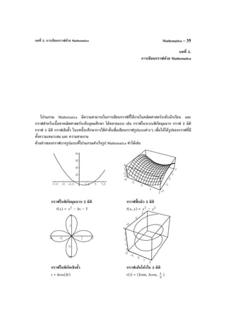
![บทที่ 3. การเขียนกราฟด้วย MathematicaMathematica – 36
3.1 การเขียนกราฟในระบบพิกัดมุมฉาก 2 มิติ
ตัวอย่าง การเขียนกราฟ y = 2
x - 3x – 7
พิมพ์ Plot[x^2-3*x-7, {x, -8, 8}]<Shift>+↵
ผลบนจอภาพ
หมายเหตุ Plot[f[x], {x, a, b}] เป็นคําสั่ง plot กราฟ y = f(x) บนช่วง [a, b]
ตัวอย่าง การเขียนกราฟ y = 2
x - 3x – 7 และ y = 2
x
พิมพ์ Plot[{2*x+3, x^2-4}, {x, -5, 5}]<Shift>+↵
ผลบนจอภาพ
หมายเหตุ Plot[{f[x], g[x], ....}, {x, a, b}] เป็นคําสั่ง plot กราฟ y = f(x) และ y = g(x) บนช่วง [a, b]
3.2 การเขียนกราฟของแผนภาพการกระจายของข้อมูล
ตัวอย่างของข้อมูลเช่น
พิมพ์ ผลบนจอภาพ
<<Graphics`Graphics`↵
เป็นคําสั่งเรียก package Graphics ขึ้นมาทํางาน
พิมพ์ ListPlot[{{2,4},{5,10},{7,25},{11,32},{15,38}}]<Shift>+↵
ผลบนจอภาพ
x y
2 4
5 10
7 25
11 32
15 38](https://image.slidesharecdn.com/bookmathcadmathemeticamatlapmaple-160531122930/85/Book-mathcad-mathematica-matlap-maple-167-320.jpg)
![บทที่ 3. การเขียนกราฟด้วย Mathematica Mathematica – 37
หมายเหตุ ListPlot[{ 1y , 2y , ...}] ใช้ เขียนกราฟคู่ลําดับ (i, iy ) , i = 1, 2, 3, ... , n
ListPlot[{{ 1x , 1y }, { 2x , 2y }, ...}] ใช้ เขียนกราฟคู่ลําดับ ( ix , iy ) , i = 1, 2, 3, ... , n
3.3 การเขียนกราฟของสมการพาราเมตริก 2 มิติ
ตัวอย่าง การเขียนกราฟของสมการ x(t) = 80t และ y(t) = –16 2
t + 80t บนช่วง 0 < t < 5
พิมพ์ ParametricPlot[{80*t,-16*t^2+80*t},{t,0,5}]<Shift>+↵
ผลบนจอภาพ
หมายเหตุ ParametricPlot[{x(t), y(t)}, {t, a, b}] เป็นคําสั่ง plot กราฟของ r(t) = (x(t), y(t)) บน
ช่วงเวลา t ตั้งแต่ a ถึง b
ParametricPlot[{{x(t), y(t)}, {f(t), g(t)}, ...}, {t, a, b}]
เป็นคําสั่ง plot กราฟของ (x(t), y(t)), (f(t), g(t)), .. บนช่วงเวลา t ตั้งแต่ a ถึง b
ตัวอย่างการเขียนกราฟพาราเมตริก 2 เส้น](https://image.slidesharecdn.com/bookmathcadmathemeticamatlapmaple-160531122930/85/Book-mathcad-mathematica-matlap-maple-168-320.jpg)
![บทที่ 3. การเขียนกราฟด้วย MathematicaMathematica – 38
3.4 การเขียนกราฟในระบบพิกัดพิกัดเชิงขั้ว
ตัวอย่างการเขียนกราฟ r = 4cos(2t)
พิมพ์ ผลบนจอภาพ
<<Graphics`Graphics`↵
เป็นคําสั่งเรียก package Graphics ขึ้นมาทํางาน
พิมพ์ PolarPlot[4*Cos[2*t],{t,0,2*Pi}]<Shift>+↵
ผลบนจอภาพ
หมายเหตุ PolarPlot[r(t), {t, a, b}] เขียนกราฟเชิงขั้ว r(t) บนช่วง [a, b]
PolarPlot3D[{ 1r (t), 2r (t), ... }, {t, a, b}] เขียนกราฟเชิงขั้ว 1r (t), 2r (t), ... บนช่วง [a, b]
ตัวอย่างเช่น
3.5 การเขียนกราฟในระบบพิกัดมุมฉาก 3 มิติ
3.5.1 กราฟพื้นผิว 3 มิติ
ตัวอย่างการเขียนกราฟพื้นผิว z = 2
x – 2
y บนช่วง [–2, 2] × [–2, 2]
พิมพ์ ผลบนจอภาพ
<<Graphics`Graphics`↵
เป็นคําสั่งเรียก package Graphics ขึ้นมาทํางาน](https://image.slidesharecdn.com/bookmathcadmathemeticamatlapmaple-160531122930/85/Book-mathcad-mathematica-matlap-maple-169-320.jpg)
![บทที่ 3. การเขียนกราฟด้วย Mathematica Mathematica – 39
พิมพ์ Plot3D[x^2-y^2,{x,-2,2},{y,-2,2}]<Shift>+↵
ผลบนจอภาพ
หมายเหตุ Plot3D[{f(x, y), {x, a, b}, {y, c,d}] เขียนกราฟพื้นผิว z = f(x, y) บนช่วง [a, b] × [c, d]
3.5.2 การเขียนกราฟแบบ contour
ตัวอย่าง การเขียนกราฟแบบ contour ของพื้นผิว z = 2
x – 2
y บนช่วง [–2, 2] × [–2, 2]
พิมพ์ ContourPlot[x^2-y^2,{x,-2,2},{y,-2,2}]<Shift>+↵
ผลบนจอภาพ
หมายเหตุ ContourPlot[{f(x, y), {x, a, b}, {y, c, d}]
เป็นคําสั่งเขียนกราฟแบบ contour ของพื้นผิว z = f(x, y) บนช่วง [a, b] × [c, d]
3.5.3 การเขียนกราฟของสมการพาราเมตริก 3 มิติ r(t) = (x(t), y(t), z(t))
ตัวอย่าง การเขียนกราฟของสมการ x(t) = sin(t), y(t) = cos(t) และ z(t) = 4
t บนช่วง 0 < t < 2π
พิมพ์ ParametricPlot3D[{Sin[t],Cos[t],t/4},{t,0,2*Pi}]<Shift>+↵
ผลบนจอภาพ](https://image.slidesharecdn.com/bookmathcadmathemeticamatlapmaple-160531122930/85/Book-mathcad-mathematica-matlap-maple-170-320.jpg)
![บทที่ 3. การเขียนกราฟด้วย MathematicaMathematica – 40
หมายเหตุ ParametricPlot3D[{x(t), y(t), z(t)}, {t, a, b}]
เป็นคําสั่ง plot กราฟของ r(t) = (x(t), y(t), z(t)) บนช่วงเวลา t ตั้งแต่ a ถึง b
3.5.4 การเขียนกราฟของสมการพาราเมตริก 3 มิติ แบบ 2 ตัวแปร
ตัวอย่าง การเขียนกราฟของสมการ
x(t, u) = cost(3 + cosu), y(t, u) = sint(3 + cosu), z(t, u) = sinu บนช่วง 0 < t < 2π และ 0 < u < 2π
พิมพ์ ParametricPlot3D[{Cos[t]*(3+Cos[u]),Sin[t]*(3+Cos[u]),Sin[u]},{t,0,2*Pi
},{u,0,2*Pi}]<Shift>+↵
ผลบนจอภาพ
หมายเหตุ ParametricPlot3D[{x(t, u), y(t, u), z(t, u)}, {t, a, b}, {u, c, d}]
เป็นคําสั่งเขียนกราฟของพื้นผิว (x(t, u), y(t, u), z(t, u)) บนช่วง [a, b] × [c, d]
ตัวอย่างของการเขียนกราฟที่มีการกําหนดรูปแบบต่าง ๆ เพื่อให้ได้รูปกราฟที่เหมาะสมและสวยงามมากขึ้น](https://image.slidesharecdn.com/bookmathcadmathemeticamatlapmaple-160531122930/85/Book-mathcad-mathematica-matlap-maple-171-320.jpg)
![บทที่ 3. การเขียนกราฟด้วย Mathematica Mathematica – 41
3.6 การเขียนกราฟของฟังก์ชันที่นิยามสูตรต่างกันในแต่ละช่วง
ตัวอย่าง การเขียนกราฟ f(x) =
≥−
<−
1x,x2
1x,1x2
ขั้นที่ 1. กําหนดสูตร f(x)
พิมพ์ f[x_]:=2*x-1/;x<1↵
f[x_]:=2-x/;x>=1<Shift>+↵
ผลบนจอภาพ
หมายเหตุ /; เป็นการกําหนดโดเมนของสูตร f(x)
พิมพ์ >= โปรแกรม Mathematica จะจัดรูปเป็น ≥
พิมพ์ <= โปรแกรม Mathematica จะจัดรูปเป็น ≤
ขั้นที่ 2. การเขียนกราฟ
พิมพ์ Plot[f[x],{x,-1,3}]<Shift>+↵
ผลบนจอภาพ
ตัวอย่าง การเขียนกราฟของ f(x) =
<
≤≤−
−<−
x2,2
2x2,x
2x,2](https://image.slidesharecdn.com/bookmathcadmathemeticamatlapmaple-160531122930/85/Book-mathcad-mathematica-matlap-maple-172-320.jpg)
![บทที่ 3. การเขียนกราฟด้วย MathematicaMathematica – 42
3.7 คําสั่งที่ใช้ในการปรับปรุงรูปแบบของกราฟ
ลักษณะ หน้าที่ ค่า Default
PlotRange กําหนดขอบเขตของพิสัยในการเขียนกราฟ Automatic
AspectRatio กําหนดสัดส่วน ความสูงต่อความกว้างของกราฟ Automatic
Frame กําหนดให้มีกรอบล้อมรอบกราฟ False
FrameLabel กําหนดให้มีคําอธิบายที่กรอบ FrameLable{xlabel,
ylabel} หรือ FrameLable{text1, text2, text3,
text4} เป็นคําอธิบายที่กรอบของรูปโดยเริ่มที่ใต้
กรอบและหมุนตามเข็มนาฬิกาไปด้านถัดไปของกรอบ
None
Axes กําหนดให้มีการแสดงแกน X, Y, Z ในกราฟ Automatic
AxesLabel กําหนดให้มีคําอธิบายที่แกน X, แกน Y ซึ่งกําหนดได้
โดย {xlabel, ylabel}
None
AxesOrigin กําหนดจุดตัดแกนว่าต้องการให้ตัดกันที่จุดใด Automatic
FrameTicks กําหนดให้มีการขีด scale ที่กรอบของกราฟ
หมายเหตุ ต้องกําหนดให้มีกรอบก่อนใช้คําสั่งนี้
Automatic
GridLines กําหนดให้มีเส้น grid ภายในกรอบของกราฟ Automatic
DisplayFunction กําหนดให้มีการแสดงกราฟหรือเก็บไว้โดยไม่แสดงผล
DisplayFunction $DisplayFunction แสดงกราฟ
DisplayFunction Identity ไม่แสดงกราฟ
$Display
Function
PlotLabel กําหนดชื่อกราฟ None
PlotStyle กําหนดลักษณะของการเขียน
เช่น PointSize[n] กําหนดขนาดของจุดที่ plot
Automatic
PlotJoined กําหนดให้มีการโยงเส้นตรงระหว่างจุดหรือไม่ False
Ticks กําหนดให้มีขีด scale ที่แกน X และ แกน Y Automatic
AxesLabel การแสดงคําอธิบายประกอบที่แกน None
Boxed กําหนดให้มีกรอบเป็นรูปกล่องล้อมรอบกราฟ True
FaceGrids การแสดงเส้น grid บนส่วน box None
HiddenSurface การแสดงพื้นผิวให้มีลักษณะเป็น solid True
Lighting การแสดงพื้นผิวที่มีสีให้มีแสง True
Mesh การแสดงพื้นผิวที่มีลักษณะเป็นร่างแห True
Shading กําหนดการแรเงาพื้นผิว True
ViewPoint กําหนดว่าจะมองกราฟในมุมใด {1.3, -2.4, 2}
หมายเหตุ การกําหนดค่าให้กับ Option ต่าง ๆ เช่น Frame → True
การพิมพ์สัญลักษณ์ลูกศร ให้พิมพ์ -> โปรแกรม Mathematica จะเปลี่ยนเป็นลูกศร → ให้เอง](https://image.slidesharecdn.com/bookmathcadmathemeticamatlapmaple-160531122930/85/Book-mathcad-mathematica-matlap-maple-173-320.jpg)
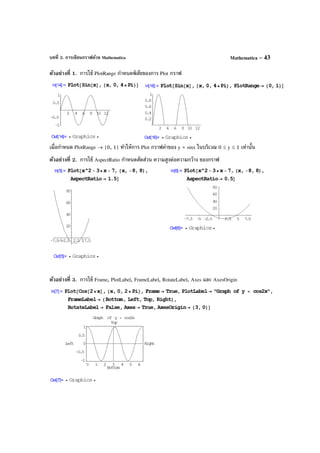
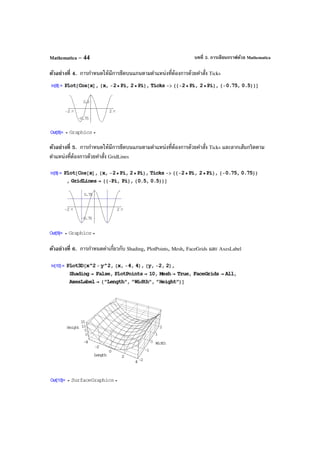
![บทที่ 3. การเขียนกราฟด้วย Mathematica Mathematica – 45
ตัวอย่างที่ 7. การเขียนกราฟหลายกรอบพร้อมกัน
line 1. เลือกใช้ package ของการเขียนกราฟ
line 2. สั่งให้เขียนกราฟรูปแรก แต่ไม่ต้องแสดงผลของกราฟ และ เก็บไว้ในตัวแปร graph1
line 3. สั่งให้เขียนกราฟรูปที่ 2 แต่ไม่ต้องแสดงผลของกราฟ และ เก็บไว้ในตัวแปร graph2
line 4. สั่งให้เขียนกราฟรูปที่ 3 แต่ไม่ต้องแสดงผลของกราฟ และ เก็บไว้ในตัวแปร graph3
line 5. สั่งให้เขียนกราฟรูปที่ 4 แต่ไม่ต้องแสดงผลของกราฟ และ เก็บไว้ในตัวแปร graph4
line 6. Show[GraphicsArray[....]] เป็นการแสดงผลของกราฟ
หมายเหตุ
Show[GraphicsArray[{g1, g2, g3, ...}] แสดงกราฟ g1, g2, g3, ... เป็นแถวตามแนวนอน
Show[GraphicsArray[{{g1}, {g2}, {g3}, ...}] แสดงกราฟ g1, g2, g3, ... เป็นแถวตามแนวดิ่ง
Show[GraphicsArray[{{g1, g2}, {g3, g4}, ...}] แสดงกราฟ g1, g2, g3, ... ในรูปแบบตาราง](https://image.slidesharecdn.com/bookmathcadmathemeticamatlapmaple-160531122930/85/Book-mathcad-mathematica-matlap-maple-176-320.jpg)
![บทที่ 3. การเขียนกราฟด้วย MathematicaMathematica – 46
ตัวอย่างที่ 8. การกําหนดค่าเกี่ยวกับจุดที่ใช้ในการเขียนกราฟ เช่นขนาดของจุด
ตัวอย่างที่ 9. การเขียนกราฟแบบโยงเส้นระหว่างจุดโดยใช้ PlotJointd → True
ตัวอย่างที่ 10. กําหนด f(x) = xsinx บนช่วง [0, π] การเขียนกราฟ f(x), f′(x) และ f′′(x) พร้อมกัน](https://image.slidesharecdn.com/bookmathcadmathemeticamatlapmaple-160531122930/85/Book-mathcad-mathematica-matlap-maple-177-320.jpg)
![บทที่ 3. การเขียนกราฟด้วย Mathematica Mathematica – 47
3.8 การเขียนกราฟของฟังก์ชันที่นิยามโดยนัยหรือกราฟของความสัมพันธ์
ตัวอย่างการเขียนกราฟของวงรี 16
x2
+ 9
y2
= 1
พิมพ์ ผลบนจอภาพ
<<Graphics`ImplicitPlot`↵
เป็นคําสั่งเรียก package ImplicitPlot ขึ้นมาทํางาน
พิมพ์ ImplicitPlot[{x^2/16+y^2/9==1},{x,-6,6},{y,-4,4}]<Shift>+↵
ผลบนจอภาพ
หมายเหตุ
ImplicitPlot[f(x, y), {x, a, b}, {y, c, d}] เขียนกราฟความสัมพันธ์ f(x, y) บนช่วง [a, b] × [c, d]
ImplicitPlot[{ 1f (x, y), 2f (x, y), ...}, {x, a, b}, {y, c, d}] เขียนกราฟความสัมพันธ์ 1f (x, y),
2f (x, y), ... บนช่วง [a, b] × [c, d]
ตัวอย่างการเขียนกราฟไฮเพอร์โบลา 16
x2
– 9
y2
= 1
การเขียนกราฟของวงกลม 2
x + 2
y = 16 และไฮเพอร์โบลา 16
x2
– 9
y2
= 1](https://image.slidesharecdn.com/bookmathcadmathemeticamatlapmaple-160531122930/85/Book-mathcad-mathematica-matlap-maple-178-320.jpg)
![บทที่ 3. การเขียนกราฟด้วย MathematicaMathematica – 48
3.9 การเขียนกราฟของสมการและการแลเงาในบริเวณที่ต้องการ
ตัวอย่างการเขียนกราฟและแรเงาพื้นที่ระหว่างเส้นโค้ง y = 2
x – x – 4 กับ y = x + 4
พิมพ์ ผลบนจอภาพ
<<Graphics`FilledPlot`↵
เป็นคําสั่งเรียก package FilledPlot ขึ้นมาทํางาน
พิมพ์ FilledPlot[{x^2-x-4,x+4},{x,-2,4},Fills->GrayLevel[0.7]]<Shift>+↵
ผลบนจอภาพ
หมายเหตุ
FilledPlot[{f(x), g(x)}, {x, a , b}] เขียนกราฟ f(x) และ g(x) บนช่วง [a, b] และแรเงาพื้นที่ด้วย
Fills→GrayLevel[0.7]] เป็นการกําหนดความเข้มของสีดําในการแรเงา
ตัวอย่างการเขียนกราฟและแรเงาพื้นที่ระหว่างเส้นโค้ง y = sinx และ y = cosx บนช่วง [0, 4
5π ]
ตัวอย่างการเขียนกราฟและแรเงาพื้นที่ระหว่างเส้นโค้ง y = 4 – 2
x บนช่วง [–2, 2]](https://image.slidesharecdn.com/bookmathcadmathemeticamatlapmaple-160531122930/85/Book-mathcad-mathematica-matlap-maple-179-320.jpg)
![บทที่ 3. การเขียนกราฟด้วย Mathematica Mathematica – 49
3.10 การเขียนกราฟของพื้นผิวที่เกิดจากการหมุนเส้นโค้ง
ตัวอย่างการเขียนกราฟพื้นผิวที่เกิดจากการหมุน เส้นโค้ง y = x บนช่วง [0, 1] รอบแกน X
พิมพ์ ผลบนจอภาพ
<<Graphics
`SurfaceOfRevolution`↵ คําสั่งเรียก package SurfaceOfRevolution ขึ้นมาทํางาน
พิมพ์ SurfaceOfRevolution[x,{x,0,1},RevolutionAxis->{1,0,0}]<Shift>+↵
ผลบนจอภาพ
หมายเหตุ
SurfaceOfRevolution[f(x), {x, a, b}, RevolutionAxis → {1, 0, 0}] เป็นคําสั่งเขียนกราฟพื้นผิวที่เกิดจาก
การหมุนเส้นโค้ง y = f(x) บนช่วง [a, b]
RevolutionAxis → {1, 0, 0}] รอบแกน X , RevolutionAxis → {0, 1, 0}] รอบแกน Y
ตัวอย่างการเขียนกราฟพื้นผิวที่เกิดจากการหมุน เส้นโค้ง y = 2sinx บนช่วง [0, 2π] รอบแกน X](https://image.slidesharecdn.com/bookmathcadmathemeticamatlapmaple-160531122930/85/Book-mathcad-mathematica-matlap-maple-180-320.jpg)
![บทที่ 3. การเขียนกราฟด้วย MathematicaMathematica – 50
ตัวอย่างการเขียนกราฟพื้นผิวที่เกิดจากการหมุน เส้นโค้ง y = 2cosx บนช่วง [0, 4π] รอบแกน X
ตัวอย่างการเขียนกราฟพื้นผิวที่เกิดจากการหมุน เส้นโค้ง y = 2cosx บนช่วง [0, 4π] รอบแกน Z](https://image.slidesharecdn.com/bookmathcadmathemeticamatlapmaple-160531122930/85/Book-mathcad-mathematica-matlap-maple-181-320.jpg)
![บทที่ 4. การใช้งานเบื้องต้นเกี่ยวกับโปรแกรม Mathematica Mathematica – 51
บทที่ 4.
การใช้งานเบื้องต้นเกี่ยวกับโปรแกรม Mathematica
ในบทนี้จะเป็นการใช้งานเบื้องต้นเกี่ยวกับโปรแกรมสําเร็จรูป Mathematica เช่นการพิมพ์สูตร การนําสูตร
เก่ากลับมาใช้ใหม่ การอ้างถึงผลลัพธ์เพื่อนํากลับมาใช้ใหม่ การบันทึกแฟ้ ม การเปลี่ยนแปลงขนาดตัวแปร
ตัวเลข การใช้งาน window ต่าง ๆ ของ Mathematica
4.1 การกําหนดผลการคํานวณให้แสดงผลลัพธ์ตามที่ต้องการ
โปรแกรม Mathematica สามารถกําหนดการแสดงผลการคํานวณได้หลายแบบเช่น
ตัวอย่างการคํานวณ คําอธิบาย
เมื่อไม่กําหนดเงื่อนไขการแสดงผล
โปรแกรมจะแสดงผลในรูปแบบ
เศษส่วน
มี . ท้ายสูตร เป็นการบังคับให้
แสดงผลเป็นเลขทศนิยม
มี //N ท้ายสูตร เป็นการบังคับให้
แสดงผลเป็นเลขทศนิยม
N[ สูตร, k] คําสั่งแสดงผลเป็นเลข
ทศนิยมที่มีเลขนัยสําคัญ k ตัว
NumberForm[ สูตร, k] คําสั่งแสดงผล
เป็นเลขทศนิยมที่มีเลขนัยสําคัญ k ตัว
ScientificForm[x, k]
แสดงผลเป็น N × m
10 โดย N มี
ตัวเลขนัยสําคัญ k ตัว
EngineeringForm[x, k] แสดงผลเป็น
N × m
10 โดย N มีตัวเลขนัยสําคัญ k
ตัว และ 3 หาร m ลงตัว](https://image.slidesharecdn.com/bookmathcadmathemeticamatlapmaple-160531122930/85/Book-mathcad-mathematica-matlap-maple-182-320.jpg)
![บทที่ 4. การใช้งานเบื้องต้นเกี่ยวกับโปรแกรม MathematicaMathematica – 52
4.2 การนําผลการคํานวณเก่ามาใช้ใน Line input ใหม่
การนําผลการคํานวณเก่าที่เคยคํานวณไว้แล้วกลับมาใช้ใหม่ มีวิธีทําดังนี้
วิธีที่ 1. ใช้การอ้างถึงด้วยสัญลักษ์ %, %%, %%% , ... และ %k
% ผลการคํานวณล่าสุดย้อนหลัง 1 ขั้นตอน
%% ผลการคํานวณล่าสุดย้อนหลัง 2 ขั้นตอน
%%% ผลการคํานวณล่าสุดย้อนหลัง 3 ขั้นตอน
:
%k ผลการคํานวณจาก Output ตัวที่ k
ตัวอย่างเช่น
ใน Input line[3] 5 + % คือการบวก 5 ด้วยผลลัพธ์ล่าสุดจาก Out[2]
ใน Input line[4] 35 + %% คือการบวก 5 ด้วยผลลัพธ์ย้อนหลัง 2 ขั้นตอน
ซึ่งเป็นผลที่ได้จาก Out[2]
ใน Input line[5] 5 + %2 คือการบวก 5 ด้วยผลลัพธ์จาก Out[2]
วิธีที่ 2. ใช้การอ้างถึงด้วย Out[k] หมายถึงผลการคํานวณใน Out[k]
ตัวอย่างเช่น
ใน Input line[5] 5 + Out[1] คือการบวก 5 ด้วยผลลัพธ์ที่ได้จาก Out[1]
4.3 การ copy สูตร และ การ paste สูตร
การทํางานใน window notebook ของ Mathematica มีสิ่งต่าง ๆ ที่เกิดขึ้นระหว่างการทํางาน จากตัวอย่าง
ต่อไปนี้ มีบริเวณที่สําคัญดังนี้
1. สัญลักษณ์ที่บอกว่าเรากําลังทํางานใน Window notebook ของ Mathematica
2. ชื่อแฟ้ มข้อมูล notebook(*.nb) ของ Mathematica ในตัวอย่างนี้ชื่อว่า test.nb
ในกรณีที่เข้าใหม่และยังไม่ได้บันทึกแฟ้ ม Mathematica จะตั้งชื่อชั่วคราวว่า Untitled
3. การนําแฟ้ มเก่ามาแก้ไข หากยังไม่ได้บันทึก Mathematica จะเตือนเราด้วยเครื่องหมายดอกจันเหนือชื่อ
4. Line Input[...] เป็นบริเวณที่เราพิมพ์คําสั่งต่าง ๆ เพื่อการคํานวณ
5. สัญลักษณ์วงเล็บที่คลุม Line Input[...] ภายในสัญลักณ์แบบนี้เราสามารถแก้ไขสูตรในบรรทัดนั้นและสั่ง
คํานวณใหม่ได้ (หมายเหตุ เมื่อแก้ไขและสั่งคํานวณ Mathematica จะถือว่า Input Line นั้นเป็น Input
Line ใหม่ล่าสุด ขอให้สังเกตที่หมายเลข Input Line[...])](https://image.slidesharecdn.com/bookmathcadmathemeticamatlapmaple-160531122930/85/Book-mathcad-mathematica-matlap-maple-183-320.jpg)
![บทที่ 4. การใช้งานเบื้องต้นเกี่ยวกับโปรแกรม Mathematica Mathematica – 53
6. สัญลักษณ์วงเล็บที่คลุม Line Input[...] และ Output Line[...] ชุดเดียวกัน โดยจําแนกย่อยเป็น
7. ส่วนของ Input Line
8. ส่วนของ Output Line (หมายเหตุ ในส่วนของ Output Line จะแก้ไขสูตรไม่ได้)
การ Copy สูตรมีขั้นตอนดังนี้
ขั้นที่ 1. คลิกเมาส์ที่วงเล็บหมายเลข 5.
จะขึ้นแถบสีดําดังรูป
ทําการ copy โดยการกด <Ctrl> + C
ขั้นที่ 2. คลิกเมาส์ในที่ว่าง ๆ ใต้บรรทัด Out[2]
กด <Ctrl> + V จะเป็น paste สิ่งที่เรา copy ไว้เพื่อจะได้ทําการแก้ไขเป็น Input Line ใหม่ต่อไป
4.3 การบันทึกแฟ้ ม Notebook.nb
จากตัวอย่างการทํางานใน Window Notebook
การ save แฟ้ มข้อมูลมีขั้นตอนดังนี้
ขั้นที่ 1. คลิกคําสั่ง File
ขั้นที่ 2. เลือกคําสั่งย่อย Save
จะได้เมนูย่อยของการบันทึกแฟ้มข้อมูล
ขั้นที่ 3. พิมพ์ชื่อแฟ้ มเช่น Newfile แล้วคลิกแป้ น Save
4.4 การเปิ ดแฟ้ ม Notebook.nb
ขณะทํางานใน Window Notebook
การเปิดแฟ้ มข้อมูลมีขั้นตอนดังนี้](https://image.slidesharecdn.com/bookmathcadmathemeticamatlapmaple-160531122930/85/Book-mathcad-mathematica-matlap-maple-184-320.jpg)
![บทที่ 4. การใช้งานเบื้องต้นเกี่ยวกับโปรแกรม MathematicaMathematica – 54
ขั้นที่ 1. คลิกคําสั่ง File
ขั้นที่ 2. เลือกคําสั่งย่อย Open
จะได้เมนูย่อยของการเปิดแฟ้ มข้อมูล
ขั้นที่ 3. พิมพ์ชื่อแฟ้ มเช่น Newfile แล้วคลิกแป้ น Open
จะได้แฟ้ มเก่าที่บันทึกไว้เพื่อจะได้ทํางานต่อไป
ข้อสังเกต ตรงหมายเลข 1. และ 2. ไม่มีคําว่า Ln[...] และ Out[...] เหตุผลก็คือ เมื่อเปิดแฟ้ ม Notebook เข้า
มาใหม่ โปรแกรม Mathematica ยังไม่เติมหมายเลข Input Line และ Output Line ให้
การสั่งให้โปรแกรมที่เปิดขึ้นมาใหม่ ทําการคํานวณใหม่มีขั้นตอนดังนี้
ขั้นที่ 1. กด <Ctrl> + A
เพื่อเลือกคํานวณใหม่ทั้งแฟ้ ม
ขั้นที่ 2. คลิกที่เมนู Kernel
เลือกเมนูย่อย Evaluation
เลือกเมนูย่อยของ Evaluation คือ Evaluate Cells
จอภาพจะเปลี่ยนแปลงไปเป็นดังนี้](https://image.slidesharecdn.com/bookmathcadmathemeticamatlapmaple-160531122930/85/Book-mathcad-mathematica-matlap-maple-185-320.jpg)
![บทที่ 4. การใช้งานเบื้องต้นเกี่ยวกับโปรแกรม Mathematica Mathematica – 55
4.5 ฟังก์ชันทางคณิตศาสตร์และฟังก์ชันอื่น ๆ ที่สําคัญ
โปรแกรม Mathematica มีฟังก์ชันทางคณิตศาสตร์ดังนี้
ฟังก์ชัน ความหมายและตัวอย่างการใช้งาน
Abs[x] ค่าสัมบูรณ์ของ x หรือ ค่าสัมบูรณ์ของจํานวนเชิงซ้อน a + bi
หมายเหตุ กด <Esc>ii<Esc> จึงจะได้สัญลักษณ์
Arg[a + bi] ค่าอาร์กิวเมนต์ของจํานวนเชิงซ้อน a + bi
Re[z], Im[z]
Conjugate[z]
ส่วนจริง ส่วนจินตภาพ และ ค่าสังยุค ของ z
Exp[x] เอกซ์โพเนนเชียลฟังก์ชัน ( x
e )
Ceiling[x] จํานวนเต็มที่เล็กที่สุดที่มีค่ามากกว่าหรือเท่ากับ x
Round[x] การปัดเศษจํานวนจริง x ให้เป็นตัวเลขจํานวนเต็มที่ใกล้ที่สุด
Floor[x] จํานวนเต็มที่ใหญ่ที่สุดที่มีค่าน้อยกว่าหรือเท่ากับ x
Log[x] Log[x] คือ ln(x) ค่าลอกาลิทึมฐาน e
Log[b, x] xlogb ค่าลอกาลิทึมฐาน b](https://image.slidesharecdn.com/bookmathcadmathemeticamatlapmaple-160531122930/85/Book-mathcad-mathematica-matlap-maple-186-320.jpg)
![บทที่ 4. การใช้งานเบื้องต้นเกี่ยวกับโปรแกรม MathematicaMathematica – 56
Mod[x, y] เศษเหลือจากการหาร x ด้วยจํานวนเต็ม y
Sign[x] เท่ากับ +1 ถ้า x > 0 และเท่ากับ –1 ถ้า x < 0
Sqrt[x] รากที่ 2 ของ x
Sin[x], Cos[x]
Tan[x], Sec[x]
Csc[x], Cot[x]
ฟังก์ชันตรีโกณมิติ
ArcSin[x]
ArcCos[x]
ArcTan[x]
ArcSec[x]
ArcCsc[x]
ArcCot[x]
ฟังก์ชันตรีโกณมิติผกผัน
Sinh[x], Cosh[x]
Tanh[x], Sech[x]
Csch[x], Coth[x]
ฟังก์ชันไฮเพอร์โบลิก
ArcSinh[x]
ArcCosh[x]
ArcTanh[x]
ArcSech[x]
ArcCsch[x]
ArcCoth[x]
ฟังก์ชันไฮเพอร์โบลิกผกผัน](https://image.slidesharecdn.com/bookmathcadmathemeticamatlapmaple-160531122930/85/Book-mathcad-mathematica-matlap-maple-187-320.jpg)
![บทที่ 4. การใช้งานเบื้องต้นเกี่ยวกับโปรแกรม Mathematica Mathematica – 57
คําสั่งเกี่ยวกับการจัดรูปพีชคณิต
ฟังก์ชัน ความหมายและตัวอย่างการใช้งาน
Apart[f(x)] เขียนเศษส่วนของพหุนามในรูปแบบผลบวกของเศษส่วนย่อย
Together[f(x)] รวมเทอมผลบวกของเศษส่วนย่อยให้อยู่ในรูปพหุนาม )x(q
)x(p
Simplify[f(x)] จัดรูปแบบพีชคณิตให้เป็นรูปแบบอย่างง่าย
Expand[f(x)]
ExpandAll[f(x)]
กระจายสูตรของฟังก์ชัน
Expand[f(x), Trig -> True] กระจายสูตรของฟังก์ชันตรีโกณมิติ
กระจายสูตรของฟังก์ชันทุกเทอมที่ปรากฏ
ComplexExpand
[f(x)]
กระจายสูตรของฟังก์ชันเชิงซ้อน](https://image.slidesharecdn.com/bookmathcadmathemeticamatlapmaple-160531122930/85/Book-mathcad-mathematica-matlap-maple-188-320.jpg)
![บทที่ 4. การใช้งานเบื้องต้นเกี่ยวกับโปรแกรม MathematicaMathematica – 58
Collect[f(x)] จัดรูปแบบพีชคณิตโดยการกระจายตามพจน์ของตัวแปรที่กําหนด
Factor[f(x)] แยกตัวประกอบ
Factor[f(x),Trig -> True] แยกตัวประกอบฟังก์ชันตรีโกณมิติ
Cancel[f(x)] หาผลหารของพหุนาม
Denominator[f(x)] ใช้ในการหาพหุนามส่วนที่เป็นตัวส่วนของ f(x)
Numerator[f(x)] ใช้ในการหาพหุนามส่วนที่เป็นตัวเศษของ f(x)
คําสั่งเกี่ยวกับผลบวก และ ผลคูณ
ฟังก์ชัน ความหมายและตัวอย่างการใช้งาน
1. Sum[f(i), {i, a, b}]
2. Sum[f(i), {i, a, b, c}]
3. Sum[f(i, j), {i, a, b,
c}, {j, d, e, k}]
1. หาผลรวม f(i) โดย i เปลี่ยนค่า จาก a ถึง b
2. หาผลรวม f(i) โดย i เปลี่ยนค่า จาก a ถึง b เพิ่มค่าครั้งละ c
3. หาผลรวม f(i, j)
โดย i เปลี่ยนค่า จาก a ถึง b เพิ่มค่าครั้งละ c
และ j เปลี่ยนค่าจาก d ถึง e เพิ่มค่าครั้งละ k](https://image.slidesharecdn.com/bookmathcadmathemeticamatlapmaple-160531122930/85/Book-mathcad-mathematica-matlap-maple-189-320.jpg)
![บทที่ 4. การใช้งานเบื้องต้นเกี่ยวกับโปรแกรม Mathematica Mathematica – 59
1. Product[f(x), {x,a,b}
2. Product[f(x),{x,a,b,c}
3. Product[f(x, y),
{x, a, b, c}, {j, d, e, k}
1. หาคูณ f(x) โดย x เปลี่ยนค่า จาก a ถึง b
2. หาผลคูณ f(x) โดย x เปลี่ยนค่า จาก a ถึง b เพิ่มค่าครั้งละ c
3. หาผลคูณ f(x, y)
โดย x เปลี่ยนค่า จาก a ถึง b เพิ่มค่าครั้งละ c
และ y เปลี่ยนค่าจาก d ถึง e เพิ่มค่าครั้งละ k
คําสั่งเกี่ยวกับ ฟังก์ชัน ลิมิต อนุพันธ์ และ อินทิเกรต
ฟังก์ชัน ความหมายและตัวอย่างการใช้งาน
f[x_]:=....
f[x]/.x→a
f[a]
f[x_]:=......เป็นการกําหนดสูตรฟังก์ชัน
คํานวณค่า f(a) (หมายเหตุ → ได้จากการพิมพ์ – และ >)
f[a] คําสั่งคํานวณค่า f(a)
Composition[f, g, ...][x]
Nest[f, x, n]
ฟังก์ชันประกอบของ f, g, ...
ฟังก์ชันประกอบ ( f...ff )(x) n ครั้ง
ตัวอย่างเช่น](https://image.slidesharecdn.com/bookmathcadmathemeticamatlapmaple-160531122930/85/Book-mathcad-mathematica-matlap-maple-190-320.jpg)
![บทที่ 4. การใช้งานเบื้องต้นเกี่ยวกับโปรแกรม MathematicaMathematica – 60
Limit[f[x], x→a]
Limit[f[x], x→a ,
Direction→–1]
Limit[f[x], x→a ,
Direction→1]
หมายถึง )x(flim
ax→
, )x(flim
ax +→
, )x(flim
ax −→
ตามลําดับ
1. f′[x], f′′[x], f′′′[x], ...
2. D[f, x]
3. D[f, {x, k}]
4. Dt[f, x]
1. f′(x), f′′(x), f′′′(x), ... ตามลําดับ
2. อนุพันธ์ หรืออนุพันธ์ย่อยของ f เทียบกับ x
3. อนุพันธ์ หรืออนุพันธ์ย่อยอันดับ k ของ f เทียบกับ x
4. ค่าอนุพันธ์ของฟังก์ชันนิยามโดยนัย
หมายเหตุ dx
dy
yx3xy2)yx(
dx
d 22332
+=
1. Integrate[f[x], x]
2. Integrate[f[x],{x,a,b}]
3.
NIntegrate[f[x],{x,a,b}]
1. fdx∫
2. dx)x(f
b
a
∫
3. การประมาณค่า dx)x(f
b
a
∫](https://image.slidesharecdn.com/bookmathcadmathemeticamatlapmaple-160531122930/85/Book-mathcad-mathematica-matlap-maple-191-320.jpg)
![บทที่ 4. การใช้งานเบื้องต้นเกี่ยวกับโปรแกรม Mathematica Mathematica – 61
คําสั่งเกี่ยวกับการคํานวณคณิตศาสตร์ขั้นสูง
ฟังก์ชัน ความหมายและตัวอย่างการใช้งาน
LaplaceTransform[f[x], x,
s]
ผลการแปลงลาปลาซของ F(s)
InverseLaplaceTransform
[F[s], s, x]
ผลการแปลงลาปลาสผกผันของ F(s)
Series[f[x], {x, a, n}] พหุนามเทย์เลอร์ของ f รอบจุด x = a ดีกรีไม่เกิน n
คําสั่งในการหารากสมการ และ ผลเฉลยของสมการเชิงอนุพันธ์
ฟังก์ชัน ความหมายและตัวอย่างการใช้งาน
Solve[equ1==equ2]
Solve[{equ1==equ2,
equ3==equ4,...}]
หารากของสมการ equ1 = equ2
หาผลเฉลยของระบบสมการ equ1 = equ2, equ3 = equ4, ...](https://image.slidesharecdn.com/bookmathcadmathemeticamatlapmaple-160531122930/85/Book-mathcad-mathematica-matlap-maple-192-320.jpg)
![บทที่ 4. การใช้งานเบื้องต้นเกี่ยวกับโปรแกรม MathematicaMathematica – 62
NSolve[equ1==equ2]
NSolve[{equ1==equ2,
equ3==equ4,...}]
หารากของสมการ equ1 = equ2
หาผลเฉลยของระบบสมการ equ1 = equ2, equ3 = equ4, ...
NRoots[equ1==equ2, x] หารากของสมการ equ1 = equ2
FindRoot[equ1==equ2,
{x, 0x }]
หารากของสมการพหุนาม equ1 = equ2 โดยมีจุดเริ่มต้นของการ
ประมาณค่ารากที่ x = 0x
Reduce[equ1==equ2] ค้นหาความเป็นไปได้ของผลเฉลยของสมการ
Eliminate[equ1==equ2
&& equ1==equ2, ตัวแปร
ที่ต้องการ]
ขจัดตัวแปรอื่น ๆ ทิ้งไปจากระบบสมการ ให้เหลือไว้เฉพาะตัว
แปรที่ต้องการ
DSolve[equ1,y[x],x] หาผลเฉลยของสมการเชิง
อนุพันธ์](https://image.slidesharecdn.com/bookmathcadmathemeticamatlapmaple-160531122930/85/Book-mathcad-mathematica-matlap-maple-193-320.jpg)
![บทที่ 5. การเขียนโปรแกรมด้วยคําสั่งของ MathematicaMathematica – 64
พิมพ์ ผลบนจอภาพ
a:=3;↵
หมายเหตุ 1. กด ↵ เพื่อขึ้น
บรรทัดใหม่ โดยไม่คํานวณ
2. สัญลักษญ์ ln[..] ยังไม่มี
เพราะว่ายังไม่ได้สั่งคํานวณ
ข้อสังเกต 1. มี * ที่ชื่อ Untiled-1*
2. Curser รอที่บรรทัดถัดไป โดยยังไม่คํานวณ
b:=4;↵
c:=5;↵
s:=(a+b+c)/2;↵
area:=Sqrt[s*(s–a)*(s–b)*(s–
c)];↵
area<Shift>+↵
ข้อสังเกต
1. ln[2] คือ b:=4;
ln[3] คือ c:=5;
:
ln[6] คือ area
ไม่แสดงสัญลักษญ์ line in ออกมา ผลการคํานวณที่ได้ คือ area มีค่าเท่ากับ 6
ทดลองเปลี่ยนค่า a, b, c ใหม่เป็น a:=5, b:=12, c:=13 แล้วกด <Shift>+↵ จะได้ผลการคํานวณใหม่ดังนี้
ข้อสังเกต 1. ได้ผลการคํานวณใหม่เป็น area = 30
2. หมายเลขของ Line In และ Line Out เปลี่ยนแปลงไปจากเดิม
การบันทึกโปรแกรม
ขั้นที่ 1. คลิกที่คําสั่ง FileSave
ขั้นที่ 2. เลือกบันทึกชื่อตามต้องการ (สมมติต้องการบันทึกชื่อเป็น Findarea)](https://image.slidesharecdn.com/bookmathcadmathemeticamatlapmaple-160531122930/85/Book-mathcad-mathematica-matlap-maple-195-320.jpg)
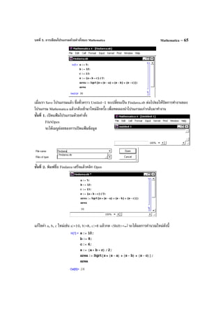
![บทที่ 5. การเขียนโปรแกรมด้วยคําสั่งของ MathematicaMathematica – 66
โปรแกรมที่ 2. การหาพื้นที่สามเหลี่ยมเมื่อกําหนดพิกัดจุดยอด 3 จุด
หมายเหตุ เมื่อกําหนดจุดยอดของสามเหลี่ยม ABC มาให้ A( 0x , 0y ), B( 1x , 1y ), C( 2x , 2y )
พื้นที่สามเหลี่ยม = 2
1 | det(
0202
0101
yyxx
yyxx
−−
−−
)| = 2
1 |( 1y – 0y )( 2x – 0x ) – ( 1x – 0x )( 2y – 0y )|
โปรแกรมการหาพื้นที่สามเหลี่ยมเมื่อกําหนดพิกัดจุดยอด 3 จุด
คําสั่งต่าง ๆ ที่ควรทราบเพื่อใช้ในการเขียนโปรแกรมของ Mathematica
คําสั่ง รูปแบบและหน้าที่
Print[...] ใช้พิมพ์ ข้อความ ตัวแปร
Do Do[คําสั่ง, {imax}] ทํางานที่กําหนดซํ้า imax ครั้ง
Do[คําสั่ง(i), {i, imax}] ทํางานที่กําหนดซํ้าตามค่าของ i ตั้งแต่ 1 ถึง
imax และ i เพิ่มค่าครั้งละ 1
Do[คําสั่ง(i), {i, imax, d}] ทํางานที่กําหนดซํ้าตามค่าของ i ตั้งแต่ 1 ถึง
imax และ i เพิ่มค่าครั้งละ d
Do[คําสั่ง(i, j), {i, imax}, {j, jmax] ทํางานที่กําหนดซํ้าตามค่าของ i
ตั้งแต่ 1 ถึง imax และ i เพิ่มค่าครั้งละ 1 และ j ตั้งแต่ 1 ถึง jmax และ j
เพิ่มค่าครั้งละ 1](https://image.slidesharecdn.com/bookmathcadmathemeticamatlapmaple-160531122930/85/Book-mathcad-mathematica-matlap-maple-197-320.jpg)
![บทที่ 5. การเขียนโปรแกรมด้วยคําสั่งของ Mathematica Mathematica – 67
While While[เงื่อนไข 1., คําสั่ง 1.]
ถ้า เงื่อนไข 1. เป็นจริง ให้ทํางานตามคําสั่ง 1.
For For[start, test, incr, body]
start การกําหนดค่าตัวแปรเริ่มต้น
test เงื่อนไขในการทํางาน ถ้า เงื่อนไข เป็นเท็จ ให้ออกจากลูป For
incr การเพิ่มค่าของตัวแปร
body กลุ่มคําสั่งของการทํางาน
If If[test, command1, command2] เมื่อ test คือ เงื่อนไข
ถ้า เงื่อนไข test เป็นจริง ให้ทํา command1
ถ้า เงื่อนไข test เป็นเท็จ ให้ทํา command2
โปรแกรมที่ 3. การหาราก f(x) = 0 โดยใช้สูตรของนิวตัน
)x(f
)x(f
xx
n
'
n
n1n −=+ เมื่อกําหนดค่าเริ่มต้น 0x
ตัวอย่าง การหารากของสมการ f(x) = 2
x – 2, 0x = 1](https://image.slidesharecdn.com/bookmathcadmathemeticamatlapmaple-160531122930/85/Book-mathcad-mathematica-matlap-maple-198-320.jpg)
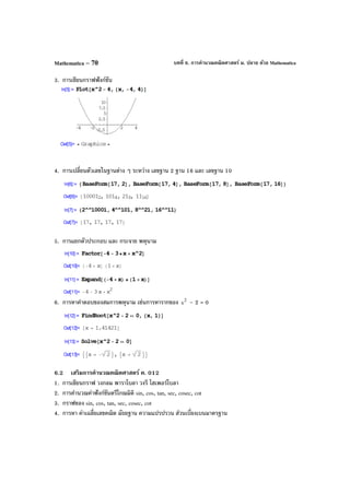
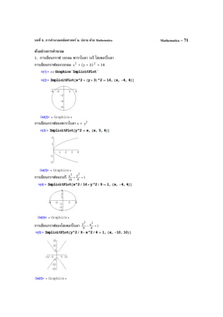
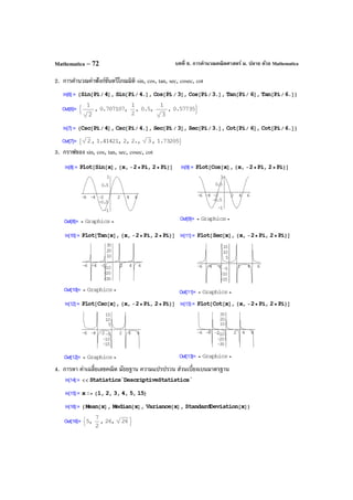
![บทที่ 6. การคํานวณคณิตศาสตร์ ม. ปลาย ด้วย MathematicaMathematica – 74
3. กราฟของฟังก์ชันตรีโกณมิติผกผัน
4. การคํานวณเกี่ยวกับเมทริกซ์
การบวกเมทริกซ์ การคูณเมทริกซ์ สเกลาร์คูณเมทริกซ์ ค่ากําหนดของเมทริกซ์
การหาผลเฉลยของระบบสมการ 2x + 3y = 2
5x + 8y = 1
หมายเหตุ ถ้า x เคยมีการกําหนดค่าไว้แล้ว ต้องใช้คําสั่ง Clear[x] เพื่อยกเลิกตัวแปร x](https://image.slidesharecdn.com/bookmathcadmathemeticamatlapmaple-160531122930/85/Book-mathcad-mathematica-matlap-maple-205-320.jpg)
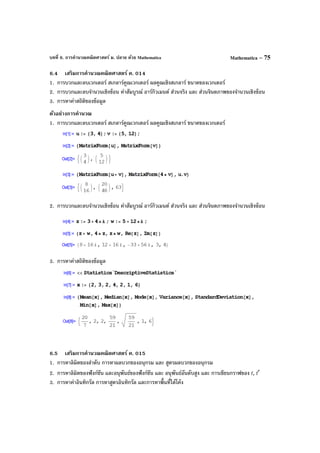
![บทที่ 6. การคํานวณคณิตศาสตร์ ม. ปลาย ด้วย MathematicaMathematica – 76
ตัวอย่างการคํานวณ
1. การหาลิมิตของลําดับ การหาผลบวกของอนุกรม และ สูตรผลบวกของอนุกรม
หมายเหตุ สัญลักษณ์ → ได้จากการพิมพ์ –>
สัญลักษณ์ ∞ ได้จากการพิมพ์ [Infinity]
หรือ <Esc>inf<Esc>
2. การหาลิมิตของฟังก์ชัน อนุพันธ์ของฟังก์ชัน และ อนุพันธ์อันดับสูง และ การเขียนกราฟของ f, f′
3. การหาค่าอินทิกรัล การหาสูตรอินทิกรัล และการหาพื้นที่ใต้โค้ง](https://image.slidesharecdn.com/bookmathcadmathemeticamatlapmaple-160531122930/85/Book-mathcad-mathematica-matlap-maple-207-320.jpg)
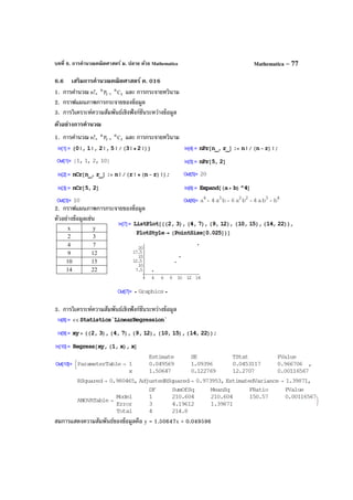
![บทที่ 6. การคํานวณคณิตศาสตร์ ม. ปลาย ด้วย MathematicaMathematica – 78
6.7 Mathematica กับการเฉลยข้อสอบคณิตศาสตร์ Entrance
ข้อสอบ Entrance สามารถหาคําตอบได้ด้วยโปรแกรม Mathematica ตัวอย่างเช่น
ข้อสอบคณิตศาสตร์ 1. มีนาคม 2546 ข้อ 18.
0x
lim
→ 3
x
1 [ x1+ – x1− – )x1)(x1( 2
−+ + )x1)(x1( 2
−− ] มีค่าเท่ากับข้อใดต่อไปนี้
1. 0 2. 4
1
3. 2
1 4. 1
การคํานวณด้วย Mathematica
เพราะฉะนั้นตอบข้อ 3.
ข้อสอบคณิตศาสตร์ 2. มีนาคม 2546 ข้อ 11.
ถ้า xsin1
1
−
+ xsin1
1
+
= 8 โดยที่ π < x <
2
3π แล้ว sin x + cos2x + tan3x มีค่าเท่ากับข้อใดต่อไปนี้
1. 2
13 −
2. 2
13 +
3. 2
13 −−
4. 2
13 +−
การคํานวณด้วย Mathematica
เพราะฉะนั้นตอบข้อ 3.
ข้อสอบคณิตศาสตร์ 1. มีนาคม 2545 ข้อ 2.
2
sin−
1 +
2sin2 –
3sin2 + ... –
89sin2 +
90sin2 มีค่าเท่ากับเท่าใด
การคํานวณด้วย Mathematica
เพราะฉะนั้น 2
sin−
1 +
2sin2 –
3sin2 + ... –
89sin2 +
90sin2 มีค่าเท่ากับ 0.5](https://image.slidesharecdn.com/bookmathcadmathemeticamatlapmaple-160531122930/85/Book-mathcad-mathematica-matlap-maple-209-320.jpg)
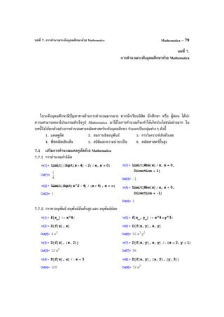
![บทที่ 7. การคํานวณระดับอุดมศึกษาด้วย MathematicaMathematica – 80
7.1.3 การคํานวณปริพันธ์ ผลการคํานวณเป็นสูตร และ ผลการคํานวณเป็นตัวเลข
7.1.4 กราฟของฟังก์ชัน f, f′ และ f′′
7.1.5 การหาผลบวกรีมันน์ (Riemann sum) เช่นผลบวกรีมันน์ของ f(x) = 2
x – 4x + 6 บนช่วง [1, 3]
เพราะฉะนั้น ค่าของ dx)6x4x(
2
3
1
+−∫ = 4.666666](https://image.slidesharecdn.com/bookmathcadmathemeticamatlapmaple-160531122930/85/Book-mathcad-mathematica-matlap-maple-211-320.jpg)
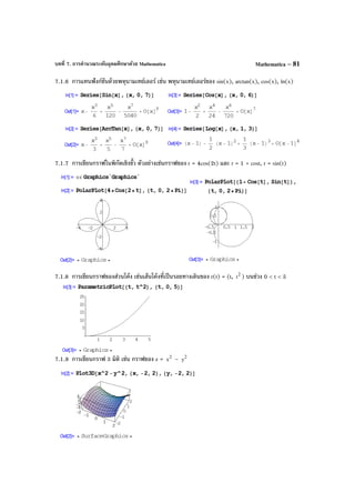
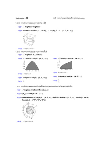
![บทที่ 7. การคํานวณระดับอุดมศึกษาด้วย Mathematica Mathematica – 83
หมายเหตุ การหมุนเส้นโค้ง f(x) = 2
)2x(4 −− บนช่วง [0, 4] รอบแกน X
จะได้อาณาบริเวณเป็นทรงกลมรัศมี r = 2
ปริมาตรที่เกิดจากการหมุน = dx)]x(f[
4
0
2
∫π = 3
32π (สูตรปริมาตรทรงกลม = 2
r
3
4 π = 3
32π )
พื้นที่ผิวที่เกิดจากการหมุน = dx)]x(f[1)x(f2
4
0
2'
∫ +π = 16π (สูตรพื้นที่ผิวทรงกลม = 4π 2
r = 16π)
7.1.13 การหาค่าตํ่าสุดของฟังก์ชัน ตัวอย่างเช่นการหาค่าตํ่าสุดของ f(x) = 2
x + 2x – 3
เพราะฉะนั้น f(–1) = –4 เป็นค่าตํ่าสุด
หมายเหตุ FindMinimun[f, {x, a}] เป็นคําสั่งหาค่าตํ่าสุดของ f(x) รอบ ๆ จุด x = a
7.2 เสริมการคํานวณเกี่ยวกับสมการเชิงอนุพันธ์ด้วย Mathematica
7.2.1 กราฟของการเคลื่อนที่แบบซิมเปิลฮาร์มอนิก
7.2.2 การหาผลเฉลยของสมการเชิงอนุพันธ์เชิงเส้น
ตัวอย่าง การหาผลเฉลยของสมการเชิงอนุพันธ์ dt
dx – 2xt = t
ตัวอย่าง การหาผลเฉลยของสมการเชิงอนุพันธ์ x′′ + 4x = 0](https://image.slidesharecdn.com/bookmathcadmathemeticamatlapmaple-160531122930/85/Book-mathcad-mathematica-matlap-maple-214-320.jpg)
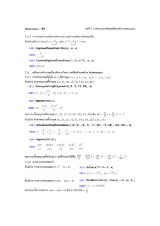
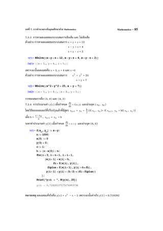
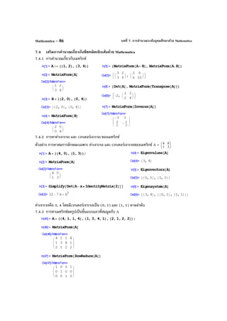
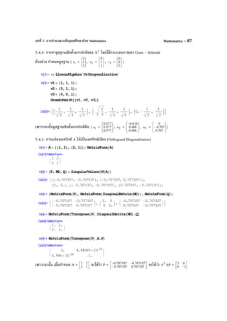
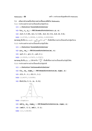
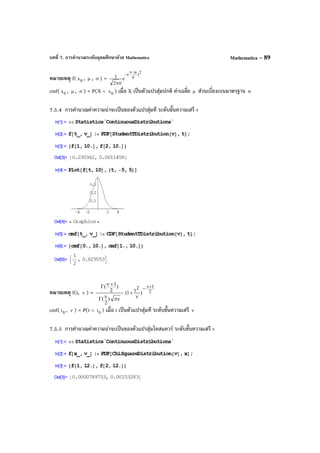
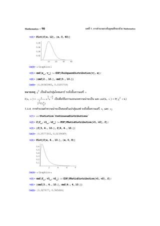
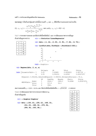
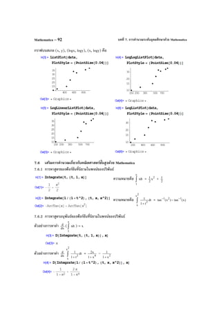
![บทที่ 7. การคํานวณระดับอุดมศึกษาด้วย Mathematica Mathematica – 93
7.6.3 กราฟของฟังก์ชันแกมมา (Gamma function) และการคํานวณค่าฟังก์ชันแกมมา
7.6.4 ฟังก์ชันเบสเซล (Bessel function) และ กราฟของฟังก์ชันเบสเซล
หมายเหตุ BesselJ[v, x] คือ ฟังก์ชันเบสเซลชนิดที่ 1 อันดับ v
BesselY[v, x] คือ ฟังก์ชันเบสเซลชนิดที่ 2 อันดับ v](https://image.slidesharecdn.com/bookmathcadmathemeticamatlapmaple-160531122930/85/Book-mathcad-mathematica-matlap-maple-224-320.jpg)
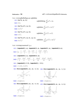
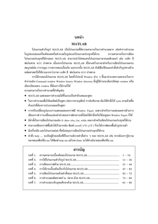
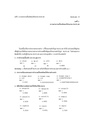
![บทที่ 1. ความสามารถเบื้องต้นของโปรแกรม MATLABMATLAB – 2
หมายเหตุ 1. asin คือ arcsin, acos คือ arccos, atan คือ arctan
2. log10 คือ ลอการิทึมฐาน 10 และ log คือ ลอการิทึมฐาน e
3. การหาค่า sin, cos, tan, ... สามารถคํานวณได้ทั้งหน่วยองศาและเรเดียน
4. ความสามารถที่จะกําหนดสูตรของฟังก์ชันใช้งานเองได้
หมายเหตุ การกําหนดสูตรฟังก์ชัน เขียนวิธีทําไว้ที่บทที่ 2.
5. สามารถสร้างตารางคํานวณค่าของฟังก์ชันได้โดยง่าย
6. สามารถเปลี่ยนหน่วยของการคํานวณได้
7. ความสามารถในการคํานวณเกี่ยวกับพหุนาม
ตัวอย่างเช่น พหุนาม p(x) = 2
x + 2x – 3 ใน MATLAB จะแทนด้วย p = [1 2 –3]
พหุนาม q(x) = 2
x + 5x + 6 ใน MATLAB จะแทนด้วย q = [1 5 6]
การบวกพหุนาม p + q ได้ ans = 2 7 3
หมายความว่า p(x) + q(x) = 2 2
x + 7x + 3
ผลของคําสั่ง roots(p) แปลว่า รากของสมการ p(x) = 0 คือ –3, 1](https://image.slidesharecdn.com/bookmathcadmathemeticamatlapmaple-160531122930/85/Book-mathcad-mathematica-matlap-maple-229-320.jpg)
![บทที่ 1. ความสามารถเบื้องต้นของโปรแกรม MATLAB MATLAB – 3
8. ความสามารถในการเขียนกราฟได้หลายแบบ
8.1 กราฟในระบบพิกัดมุมฉาก
ตัวอย่าง กราฟของ f(x) = 2x + 3 บนช่วง [–5, 5]
8.2 สามารถเขียนกราฟได้หลายเส้นพร้อมกัน
ตัวอย่าง กราฟของ f(x) = 2x + 3 กับ g(x) = 2
x – 4 บนช่วง [–5, 5]
8.3 กราฟแบบคู่ลําดับ
ตัวอย่าง กราฟของข้อมูล นํ้าหนักและส่วนสูง
นํ้าหนัก ความสูง
53 156
58 165
55 162
60 170
62 165
68 173
8.4 กราฟแท่ง (Bar graph) ของข้อมูลทางสถิติ
ตัวอย่าง กราฟของข้อมูล คะแนน และ ความถี่
คะแนน ความถี่
1 15
2 35
3 40
4 10](https://image.slidesharecdn.com/bookmathcadmathemeticamatlapmaple-160531122930/85/Book-mathcad-mathematica-matlap-maple-230-320.jpg)
![บทที่ 1. ความสามารถเบื้องต้นของโปรแกรม MATLABMATLAB – 4
8.5 กราฟในระบบพิกัดเชิงขั้ว
ตัวอย่าง กราฟรูปหัวใจ r = 3 + 2sinθ, กราฟรูปกลีบกุหลาบ r = 2cos2θ
8.6 กราฟในระบบพิกัด 3 มิติ เช่นกราฟพื้นผิว กราฟ contour
ตัวอย่าง กราฟพื้นผิวไฮเพอร์โบลิกพาราโบลอยด์ หรือพื้นผิวรูปอานม้า f(x, y) = 2
x – 2
y
8.7 สามารถปรับเปลี่ยนรูปแบบของกราฟให้เหมาะสมกับการใช้งาน
ตัวอย่าง กราฟของ f(x) = 3
x + 2
x – 9x – 9 บนช่วง [–4, 4]](https://image.slidesharecdn.com/bookmathcadmathemeticamatlapmaple-160531122930/85/Book-mathcad-mathematica-matlap-maple-231-320.jpg)
![บทที่ 1. ความสามารถเบื้องต้นของโปรแกรม MATLAB MATLAB – 5
8.8 สามารถเขียนกราฟได้หลายรูปพร้อมกัน บนกรอบที่ต่างกัน
ตัวอย่าง กราฟของอนุพันธ์อันดับต่าง ๆ ของฟังก์ชัน f(x) = 4
x บนช่วง [–4, 4]
8.9 สามารถเขียนกราฟวงกลมได้ ตัวอย่างเช่น
9. สามารถคํานวณตัวเลขในระบบฐานต่าง ๆ ได้
การเปลี่ยนแปลงค่าระหว่างเลขฐาน 10 กับ เลขฐาน 2 ตัวอย่างเช่น 1012 = 21100
การเปลี่ยนแปลงค่าระหว่างเลขฐาน 10 กับ เลขฐาน 16 ตัวอย่างเช่น 1020 = 1614
10. การคํานวณเกี่ยวกับเวกเตอร์
MATLAB สามารถหาผลบวก ผลต่าง dot product cross product และ ขนาดของเวกเตอร์ได้
การกําหนดเวกเตอร์](https://image.slidesharecdn.com/bookmathcadmathemeticamatlapmaple-160531122930/85/Book-mathcad-mathematica-matlap-maple-232-320.jpg)
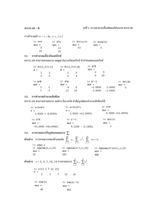
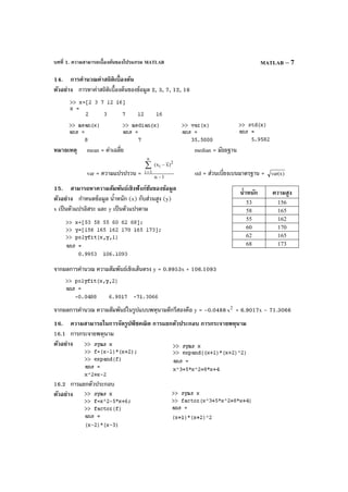
![บทที่ 1. ความสามารถเบื้องต้นของโปรแกรม MATLAB MATLAB – 9
21. ความสามารถในการหารากของสมการ f(x) = 0
ตัวอย่าง การหารากของสมการ 2
x - 2 = 0
เพราะฉะนั้นรากสมการคือ x = 1.4142 และ x = –1.4142
หมายเหตุ f = [1 0 -2] หมายถึงพหุนาม f(x) = 1 2
x + 0x + (–2) ซึ่งคือ f(x) = 2
x – 2
คําสั่ง roots(f) เป็นคําสั่งหารากของสมการ f(x) = 0
ตัวอย่าง การหารากของสมการ sinx - cosx = 0
เพราะฉะนั้น รากสมการ sinx - cosx = 0 คือ x = 4
π
22. ความสามารถในการหาผลเฉลยของระบบสมการ
22.1 การหาผลเฉลยระบบสมการเชิงเส้น
ตัวอย่าง การหาผลเฉลยของระบบสมการ
2x + y = 4
9x – 4y = 1
เพราะฉะนั้นผลเฉลยของระบบสมการคือ x = 1, y = 2
22.2 การหาผลเฉลยระบบสมการไม่เชิงเส้น
ตัวอย่าง การหาผลเฉลยของระบบสมการ
2
x + 2
y = 25 และ 3x – 4y = 0
เพราะฉะนั้นจุดตัดของวงกลม 2
x + 2
y = 25
กับเส้นตรง 3x – 4y = 0
คือ (x, y) = (4, 3), (–4, –3)
23. ความสามารถในการหาผลเฉลยของสมการเชิงอนุพันธ์
23.1 การหาผลเฉลยของสมการเชิงอนุพันธ์
ตัวอย่าง การหาผลเฉลยของสมการเชิงอนุพันธ์ x′ – x = 0
เพราะฉะนั้นผลเฉลยคือ x(t) = 1c t
e](https://image.slidesharecdn.com/bookmathcadmathemeticamatlapmaple-160531122930/85/Book-mathcad-mathematica-matlap-maple-236-320.jpg)
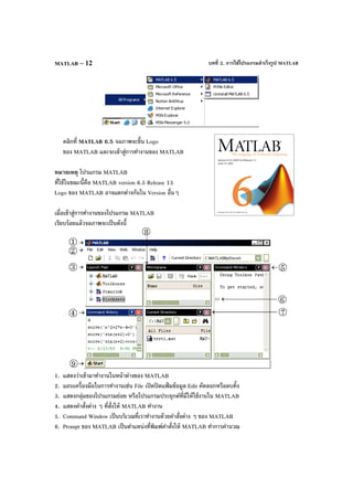
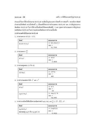
![บทที่ 2. การใช้โปรแกรมสําเร็จรูป MATLABMATLAB – 16
พิมพ์ function y=f(x);↵
พิมพ์ y=x.^2;
การ save โปรแกรม
ขั้นที่ 4. การ save โปรแกรม เลือกคําสั่ง File Save
บันทึกชื่อแฟ้ มเป็น f
เสร็จแล้วคลิกปุ่ม Save
การเรียกฟังก์ชันที่กําหนดสูตรไว้แล้วคือ f(x) = 2
x
ในโปรแกรม f.m
พิมพ์ ผลบนจอภาพ
x=4;↵
f(x)↵
x=[1;2;3];↵
f(x)↵
7. การหาค่าอินทิกรัล dx)x(f
b
a
∫ ตัวอย่างเช่น dx)4x(
2
4
1
+∫
พิมพ์ ผลบนจอภาพ
syms x↵
int(x.^2+4,1,4)↵
หมายเหตุ syms เป็นการกําหนดตัวแปรที่ต้องการคํานวณในรูปแบบสัญลักษณ์
2.3 การเขียนกราฟของฟังก์ชัน
ตัวอย่าง การเขียนกราฟของ f(x) = 2
x – 3x – 7 บนช่วง [–8, 8]
พิมพ์ ผลบนจอภาพ
x=-8:0.1:8;↵
หมายเหตุ เครื่องหมาย ; เป็นการ
กําหนดว่า ไม่ต้องแสดงผลของ
คําสั่งที่กําหนดนี้
รูปแบบ x = a : d : b หมายถึงตัวแปร x มีค่าตั้งแต่ a ถึง
b โดยมีการเพิ่มค่าครั้งละ d](https://image.slidesharecdn.com/bookmathcadmathemeticamatlapmaple-160531122930/85/Book-mathcad-mathematica-matlap-maple-243-320.jpg)
![บทที่ 2. การใช้โปรแกรมสําเร็จรูป MATLAB MATLAB – 17
y=x.^2-3*x-7;↵
หมายเหตุ ตัวแปร x เป็นตัวแปรมิติการยกกําลังสองต้อง
ใช้รูปแบบ x.^2
plot(x,y)↵
หมายเหตุ เนื่องจากคําสั่งก่อนหน้า
นี้มี ; ปิดท้ายคําสั่ง เมื่อมาถึงคําสั่ง
plot(x,y) โปรแกรม MATLAB
จึงทําการประมวลผล 3 คําสั่ง
พร้อมกันตามลําดับคือ
x=-8:0.1:8;
y=x.^2-3*x-7;
และ plot(x,y)
หมายเหตุ โปรแกรม MATLAB สามารถจัดรูปแบบการแสดงผลของกราฟได้หลายลักษณะเช่น
มีสเกลที่แกน X และ แกน Y และมี grid line กราฟแบบ scale log
2.4 การกําหนดค่าและการคํานวณเกี่ยวกับเมทริกซ์
ตัวอย่าง การกําหนด A =
−
−
35
24 และ B =
31
52
พิมพ์ ผลบนจอภาพ
A=[4,-2;-5,3]↵
หมายเหตุ , หรือ ช่องว่าง คือการ
จําแนก หลัก ; คือการจําแนกแถว
B=[2,5;1,3]↵](https://image.slidesharecdn.com/bookmathcadmathemeticamatlapmaple-160531122930/85/Book-mathcad-mathematica-matlap-maple-244-320.jpg)
![บทที่ 2. การใช้โปรแกรมสําเร็จรูป MATLABMATLAB – 18
การคํานวณค่าของเมทริกซ์ A + B, AB, 4A, 2
A , 1
A
−
, T
A , det(A)
พิมพ์ ผลบนจอภาพ
A+B↵
A*B↵
4*A↵
A^2↵
A^–1↵
หมายเหตุ inv(A) จะได้ 1
A−
A'↵
det(A)↵
การกําหนดดรรชนีล่าง (subscript) สําหรับอ้างอิงใช้งานกับสมาชิกของเมทริกซ์
พิมพ์ ผลบนจอภาพ
A(1,1)↵
A(1,1)+A(2,2)↵
หมายเหตุ A(i, j) คือ ija ของเมทริกซ์ A = nmij]a[ ×](https://image.slidesharecdn.com/bookmathcadmathemeticamatlapmaple-160531122930/85/Book-mathcad-mathematica-matlap-maple-245-320.jpg)
![บทที่ 2. การใช้โปรแกรมสําเร็จรูป MATLAB MATLAB – 19
2.5 การกําหนดค่าและการคํานวณเกี่ยวกับเวกเตอร์
ตัวอย่างเช่น u =
−
4
3 และ v =
2
1 และการหาค่า u + v, 4u, vu ⋅ และ | u |
พิมพ์ ผลบนจอภาพ
u=[-3;4]↵
v=[1;2]↵
u+v↵
4*u↵
dot(u,v)↵
norm(u)↵
2.6 การกําหนดข้อมูล
สําหรับข้อมูลที่อยู่ในรูปแบบของเวกเตอร์เช่น x =
15
8
7
5
3
2
พิมพ์ ผลบนจอภาพ
x=[2;3;5;7;8;15]↵
mean(x)↵](https://image.slidesharecdn.com/bookmathcadmathemeticamatlapmaple-160531122930/85/Book-mathcad-mathematica-matlap-maple-246-320.jpg)
![บทที่ 2. การใช้โปรแกรมสําเร็จรูป MATLABMATLAB – 20
median(x)↵
std(x)↵
var(x)↵
ใน MATLAB มีฟังก์ชันที่ช่วยคํานวณค่าทางด้านสถิติของข้อมูลดังนี้
mean(x) = ค่าเฉลี่ยเลขคณิตของข้อมูลใน x median(x) = มัธยฐานของข้อมูลใน x
var(x) = ความแปรปรวน(ตัวอย่าง) x std(x) = ส่วนเบี่ยงเบนมาตรฐาน(ตัวอย่าง) x
max(x) = ค่าสูงสุดของข้อมูลใน x min(x) = ค่าตํ่าสุดของข้อมูลใน x
range(x) = พิสัยของข้อมูลใน x
การกําหนดข้อมูลแบบแถวทําได้ดังนี้
พิมพ์ ผลบนจอภาพ
x=[2,3,5,7,8,15]↵
mean(x)↵
x(4)↵
2.7 การกําหนดข้อมูลในรูปแบบเมทริกซ์
ตัวอย่างเช่นต้องการกําหนดข้อมูล
พิมพ์ ผลบนจอภาพ
xy=[3,12;5,15;9,21;12,32]↵
x y
3 12
5 15
9 21
12 32](https://image.slidesharecdn.com/bookmathcadmathemeticamatlapmaple-160531122930/85/Book-mathcad-mathematica-matlap-maple-247-320.jpg)
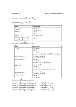
![บทที่ 2. การใช้โปรแกรมสําเร็จรูป MATLAB MATLAB – 23
พิมพ์ ผลบนจอภาพ
hex2dec('17')↵
dec2hex(23)↵
dec2bin(12)↵
bin2dec('1100')↵
2.13 การหาผลบวกในรูปแบบ ∑
=
n
1i
ix
ตัวอย่าง กําหนดข้อมูลจากตาราง
การหาค่าของ ∑
=
4
1i
ix , ∑
=
4
1i
iy , ∑
=
4
1i
2
ix , ∑
=
4
1i
2
iy , ∑
=
4
1i
iiyx
พิมพ์ ผลบนจอภาพ
x=[2 3 6 9];↵
y=[12 15 14 19];↵
sum(x)↵
sum(y)↵
sum(x.^2)↵
sum(y.^2)↵
sum(x.*y)↵
x y
2 12
3 15
6 14
9 19](https://image.slidesharecdn.com/bookmathcadmathemeticamatlapmaple-160531122930/85/Book-mathcad-mathematica-matlap-maple-250-320.jpg)
![บทที่ 2. การใช้โปรแกรมสําเร็จรูป MATLABMATLAB – 24
2.14 การสร้างตารางฟังก์ชัน
การคํานวณค่า f(x) = 2x + 4, x = 1, 2, 3, 4 ในรูปแบบตาราง
พิมพ์ ผลบนจอภาพ
x=[1;2;3;4]↵
2*x+4↵
f(x)=2*x+4;↵
f(x)↵
2.15 การคํานวณค่าเกี่ยวกับจํานวนเชิงซ้อน
ตัวอย่าง z = 3 + 4i, w = 5 – 9i การหาค่า z + w, zw, | z |, Arg(z), Re(z), Im(z) และ z
พิมพ์ ผลบนจอภาพ
z=3+4*i↵
w=5–9*i↵
z+w↵
z*w↵
abs(z)↵
angle(z)↵
หมายเหตุ angle(z) คือค่า
อาร์กิวเมนต์ของ z](https://image.slidesharecdn.com/bookmathcadmathemeticamatlapmaple-160531122930/85/Book-mathcad-mathematica-matlap-maple-251-320.jpg)
![บทที่ 2. การใช้โปรแกรมสําเร็จรูป MATLAB MATLAB – 25
real(z)↵
imag(z)↵
cong(z)↵
2.16 การหารากของสมการ f(x) = 0 ตัวอย่างเช่น การหารากของสมการ 2
x – 2 = 0
พิมพ์ ผลบนจอภาพ
f=[1 0 -2]↵
roots[f]↵
2.17 การหาผลเฉลยของระบบสมการ ตัวอย่างเช่น การหาผลเฉลยของระบบสมการ 2x + 3y = 8
x + y = 3
พิมพ์ ผลบนจอภาพ
[x y] =
solve('2*x+3*y=8','x+y=3')↵
2.18 การคํานวณค่า r
n
C และ nPr r
n
P
r
n
C = )!rn(!r
!n
−
กําหนดเป็นสูตรในโปรแกรม nCr.m ได้ดังนี้
พิมพ์ ผลบนจอภาพ
nCr(5,1)↵
nCr(5,2)↵](https://image.slidesharecdn.com/bookmathcadmathemeticamatlapmaple-160531122930/85/Book-mathcad-mathematica-matlap-maple-252-320.jpg)
![บทที่ 2. การใช้โปรแกรมสําเร็จรูป MATLAB MATLAB – 29
syms s↵
F=1/(s^2+1);↵
ilaplace(F))↵
2.20.3 การหาสูตรเทย์เลอร์ของฟังก์ชัน เช่นการหาสูตรเทย์เลอร์ของ sinx มีวิธีทําได้ 2 แบบ
พิมพ์ ผลบนจอภาพ
syms x↵
taylor(sin(x),5);↵
syms x↵
f=sin(x);↵
taylor(f,5);↵
syms x↵
f=sin(x);↵
taylor(f,8)↵
2.20.4 การแยกเศษส่วนย่อยด้วยโปรแกรม MATLAB
3x4x
6xx5x2
2
23
+−
−+− สามารถแยกเป็นผลบวก 2x + 3 + 3x
3
−
+ 1x
4
−
พิมพ์ ผลบนจอภาพ
a=[1 -4 3];↵
b=[2 -5 1 -6];↵
[r,p,k]=rersidue(b,a)↵
a = เวกเตอร์ของสัมประสิทธิ์พหุนามตัวส่วน
b = เวกเตอร์ของสัมประสิทธิ์พหุนามตัวเศษ
[r, p, k] = residue(b, a) จะทําการหารยาวและให้ค่า
k = เวกเตอร์ของสัมประสิทธิ์ส่วนที่เป็นพหุนาม](https://image.slidesharecdn.com/bookmathcadmathemeticamatlapmaple-160531122930/85/Book-mathcad-mathematica-matlap-maple-256-320.jpg)
![บทที่ 2. การใช้โปรแกรมสําเร็จรูป MATLABMATLAB – 30
p =
m
2
1
p
:
p
p
และ r =
m
2
1
r
:
r
r
เป็นค่าที่สอดคล้องกันซึ่งหมายถึง
1
1
px
r
−
+
2
2
px
r
−
+ ... +
m
m
px
r
−
การกระจาย 2x + 3 + 3x
3
−
+ 1x
4
−
เป็น
3x4x
6xx5x2
2
23
+−
−+− ทําได้ด้วยคําสั่ง [b, a] = residue(r, p, k)
พิมพ์ ผลบนจอภาพ
k=[2 3];↵
r=[3 4 ];↵
p=[3 1];↵
[b,a]=rersidue(r,p,k)↵
2.20.5 การหาผลเฉลยของสมการเชิงอนุพันธ์
ตัวอย่าง การหาผลเฉลยของสมการเชิงอนุพันธ์ y′ – 4y = 4 และ y(0) = 1
พิมพ์ ผลบนจอภาพ
dsolve('Dy–4y=4','t(0)=1')↵
ตัวอย่าง การหาผลเฉลยของสมการเชิงอนุพันธ์ y′′ + 4y = t และ y(0) = 1, y′(0) = –2
พิมพ์ dsolve('D2y+4*y=t','y(0)=1','Dy(0)=–2')↵
ผลบนจอภาพ
รูปแบบคําสั่ง dslove('สมการ', 'เงื่อนไข', 'เงื่อนไข', ...) Dy หมายถึง dt
dy
, D2y หมายถึง 2
2
dt
yd
2.20.6 การหาผลเฉลยของระบบสมการเชิงอนุพันธ์
ตัวอย่าง การหาผลเฉลยของระบบสมการเชิงอนุพันธ์ x′ + y′ = sin(t), x′ – y′ = cos(t)
พิมพ์ dsolve('Dx+Dy=sin(t)','Dx-Dy=cos(t)')↵
ผลบนจอภาพ](https://image.slidesharecdn.com/bookmathcadmathemeticamatlapmaple-160531122930/85/Book-mathcad-mathematica-matlap-maple-257-320.jpg)
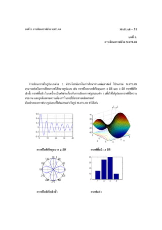
![บทที่ 3. การเขียนกราฟด้วย MATLABMATLAB – 32
3.1 การเขียนกราฟในระบบพิกัดมุมฉาก 2 มิติ
ตัวอย่าง การเขียนกราฟของ f(x) = 2x + 3 บนช่วง [0, 10] โดยใช้คําสั่ง plot
พิมพ์ ผลบนจอภาพ
x=0:0.1:10;↵
y=2*x+3;↵
plot(x,y)↵
หมายเหตุ MATLAB จะแสดง
ภาพของกราฟใน Window ใหม่
เรียกว่า Window Figure และ
ภาพใน Window นี้สามารถ
แก้ไขรูปแบบ และบันทึกเป็น
แฟ้ มข้อมูลแบบกราฟได้โดยใช้
คําสั่ง File, Save
หมายเหตุ plot(x, y) เป็นคําสั่งเขียนกราฟของเส้นโค้งหรือฟังก์ชัน y = f(x)
ตัวอย่าง การเขียนกราฟของ f(x) = 2x + 3 บนช่วง [0, 10] โดยใช้คําสั่ง ezplot
พิมพ์ ผลบนจอภาพ
ezplot('2*x+3',[0,10])↵
หมายเหตุ ezplot('f(x)', [a, b]) เป็นคําสั่งเขียนกราฟของ f(x) บนช่วง [a, b]](https://image.slidesharecdn.com/bookmathcadmathemeticamatlapmaple-160531122930/85/Book-mathcad-mathematica-matlap-maple-259-320.jpg)
![บทที่ 3. การเขียนกราฟด้วย MATLAB MATLAB – 33
ตัวอย่าง การเขียนกราฟ 2 ฟังก์ชันโดเมนเดียวกัน
ตัวอย่าง การเขียนกราฟ 2 ฟังก์ชันที่มีโดเมนต่างกัน
3.2 การเขียนกราฟขั้นบันได
การเขียนกราฟแบบขั้นบันไดของข้อมูล
พิมพ์ ผลบนจอภาพ
x=[15 35 40 10];↵
stairs(x)↵
หมายเหตุ stairs(x) เป็นคําสั่งเขียนกราฟขั้นบันไดของข้อมูลใน x
stairs(x, f(x)) เป็นคําสั่งเขียนกราฟขั้นบันไดของเส้นโค้ง y = f(x)
ตัวอย่างเช่น การเขียนกราฟแบบขั้นบันไดของ f(x) = sin(x) เมื่อ x = 0, 0.5, 1.0, 1.5, ... , 4π
No X
1 15
2 35
3 40
4 10](https://image.slidesharecdn.com/bookmathcadmathemeticamatlapmaple-160531122930/85/Book-mathcad-mathematica-matlap-maple-260-320.jpg)
![บทที่ 3. การเขียนกราฟด้วย MATLABMATLAB – 34
กราฟที่ได้คือ
3.3 การเขียนกราฟแบบ histogram
กราฟแบบ histogram เป็นกราฟแสดงการแจกแจงความถี่ของข้อมูล
hist(x, y) เป็นคําสั่งแจกแจงความถี่ของข้อมูลจาก x ตามค่าที่กําหนดจาก y แล้วแสดงผลในรูปแบบกราฟ
ตัวอย่างเช่น การแจกแจงความถี่และกราฟของคะแนนสอบจากข้อมูล 1, 4, 1, 1, 2, 2, 3, 2 , 2 และ 3
พิมพ์ ผลบนจอภาพ
data=[1 4 1 1 2 2 3 2 2 3];↵
grade=[1 2 3 4];↵
hist(data,score)↵
หมายเหตุ hist(x) จะนําข้อมูลใน x มาแจกแจงความถี่และเขียนกราฟ
ตัวอย่างเช่น
กราฟที่ได้คือ
3.4 การเขียนกราฟวงกลม
การเขียนกราฟวงกลมของข้อมูล
No X
1 15
2 35
3 40
4 10](https://image.slidesharecdn.com/bookmathcadmathemeticamatlapmaple-160531122930/85/Book-mathcad-mathematica-matlap-maple-261-320.jpg)
![บทที่ 3. การเขียนกราฟด้วย MATLAB MATLAB – 35
พิมพ์ ผลบนจอภาพ
x=[15 35 40 10];↵
pie(x)↵
หมายเหตุ pie(x) เป็นคําสั่งเขียนกราฟวงกลมของข้อมูลใน x
pie(x, explode) เป็นคําสั่งเขียนกราฟวงกลมของข้อมูลใน x
และดึงชิ้นที่กําหนดออกมา
โดยกําหนด explode = [d d d ...]
d = 0 หรือ d = 1 โดยที่ d = 1 หมายถึงให้ดึงชิ้นนั้นออกมา
ตัวอย่างเช่น
pie3(x, explode) เป็นคําสั่งเขียนกราฟวงกลมของข้อมูลใน x
และดึงชิ้นที่กําหนดออกมาโดยแสดงภาพเป็นรูปแบบ 3 มิติ
ตัวอย่างเช่น
หมายเหตุ pie(x, x == min(x)) ดึงชิ้นที่มีค่าตํ่าสุดออกมา pie(x, x == max(x)) ดึงชิ้นที่มีค่าสูงสุดออกมา
3.5 การเขียนกราฟแท่ง (Bar graph) ของข้อมูลทางสถิติ
ตัวอย่าง การเขียนกราฟของข้อมูล คะแนน และ ความถี่
พิมพ์ ผลบนจอภาพ
score=[1 2 3 4];↵
freq=[15 35 40 10];↵
bar(score,freq)↵
score frequency
1 15
2 35
3 40
4 10](https://image.slidesharecdn.com/bookmathcadmathemeticamatlapmaple-160531122930/85/Book-mathcad-mathematica-matlap-maple-262-320.jpg)
![บทที่ 3. การเขียนกราฟด้วย MATLABMATLAB – 36
หมายเหตุ bar(x, y) เป็นคําสั่งเขียนกราฟแท่งโดยมีแกนนอนเป็นข้อมูล x และ ข้อมูล y เป็นแกนตั้ง
ตัวอย่าง การเขียนกราฟแท่งโดยระบุค่าเฉพาะข้อมูล y
หมายเหตุ โปรแกรม MATLAB จะกําหนดข้อมูล x เป็น [1 2 3 ...]
3.6 การเขียนกราฟของแผนภาพการกระจายของข้อมูล
ตัวอย่างของข้อมูลเช่น
พิมพ์ ผลบนจอภาพ
x=[53 58 55 60 62 68];↵
y=[156 165 162 170 165 173];↵
plot(x,y,'*')↵
หมายเหตุ plot(x, y, '*') เป็นคําสั่ง plot กราฟแบบจุดของคู่ลําดับ ( ix , iy ) โดย plot ด้วยสัญลักษณ์ที่
กําหนดใน '...' ในตัวอย่างนี้คือ plot จุดด้วย *
x y
53 156
58 165
55 162
60 170
62 165
68 173](https://image.slidesharecdn.com/bookmathcadmathemeticamatlapmaple-160531122930/85/Book-mathcad-mathematica-matlap-maple-263-320.jpg)
![บทที่ 3. การเขียนกราฟด้วย MATLAB MATLAB – 37
3.7 การเขียนกราฟในระบบพิกัดเชิงขั้ว
ตัวอย่าง การเขียนกราฟ r = 2cos(2t)
พิมพ์ ผลบนจอภาพ
t=0:0.1:2*pi;↵
r=2*cos(2*t);↵
polar(t,r)↵
หมายเหตุ polar(r, t) เป็นคําสั่ง plot กราฟแบบในระบบพิกัดเชิงขั้ว
ตัวอย่าง การเขียนกราฟ r = 4cos(t)
พิมพ์ ผลบนจอภาพ
ezpolar('4*cos(t)',[0,2*pi])↵
หมายเหตุ ezpolar('r(t)', [a, b]) เป็นคําสั่ง plot กราฟพิกัดเชิงขั้ว r(t) บนช่วง [a, b]
3.8 การเขียนกราฟของสมการพาราเมตริก
3.8.1 กราฟพาราเมตริก 2 มิติ
ตัวอย่าง การเขียนกราฟของเส้นโค้งที่มีสมการพาราเมตริก x(t) = 80t และ y(t) = –16 2
t + 80t
บนช่วง 0 < t < 5 ขั้นตอนการเขียนกราฟของเส้นโค้งที่มีสมการพาราเมตริกเป็นดังนี้
พิมพ์ ezplot('80*t','-16*t^2+80*t',[0,5])↵](https://image.slidesharecdn.com/bookmathcadmathemeticamatlapmaple-160531122930/85/Book-mathcad-mathematica-matlap-maple-264-320.jpg)
![บทที่ 3. การเขียนกราฟด้วย MATLABMATLAB – 38
ผลบนจอภาพ
หมายเหตุ ezplot('x(t)', 'y(t)', [a, b]) เป็นคําสั่ง plot กราฟ r(t) = (x(t), y(t)) บนช่วง [a, b]
3.8.2 กราฟพาราเมตริก 3 มิติ
ตัวอย่าง การเขียนกราฟของเส้นโค้งที่มีสมการพาราเมตริก x(t) = cost, y(t) = sint และ z(t) = 4
t
บนช่วง 0 < t < 2π
พิมพ์ ezplot3('cos(t)','sin(t)','t/4',[0,2*pi])↵
ผลบนจอภาพ
หมายเหตุ
ezplot3('x(t)', 'y(t)', 'z(t)', [a, b]) เป็นคําสั่งเขียนกราฟ r(t) = (x(t), y(t), z(t)) บนช่วง [a, b]](https://image.slidesharecdn.com/bookmathcadmathemeticamatlapmaple-160531122930/85/Book-mathcad-mathematica-matlap-maple-265-320.jpg)
![บทที่ 3. การเขียนกราฟด้วย MATLAB MATLAB – 39
3.9 การเขียนกราฟพื้นผิว 3 มิติ และกราฟแบบ contour
ตัวอย่าง การเขียนกราฟพื้นผิว f(x, y) = 2
x – 2
y บนช่วง [–2, 2] × [–2, 2] และกราฟ contour
แบบที่ 1. ขั้นตอนการทํางานมีดังนี้
1. กําหนดสูตรฟังก์ชัน z = 2
x – 2
y
2. กําหนดโดเมน x เป็น [–2, 2]
3. กําหนดโดเมน y เป็น [–2, 2]
4. สร้างเมทริกซ์ของการเขียนกราฟด้วยคําสั่ง meshgrid เพื่อเป็นโดเมนของฟังก์ชัน z
5. เขียนกราฟพื้นผิว ด้วยคําสั่ง surf(z)
6. เขียนกราฟ contour ด้วยคําสั่ง contour(z)
พิมพ์ ผลบนจอภาพ
z=x.^2-y.^2;↵
x=-2:0.1:2;↵
y=-2:0.1:2;↵
[x,y]=meshgrid(x,y)↵
surf(z)↵
contour(z)↵](https://image.slidesharecdn.com/bookmathcadmathemeticamatlapmaple-160531122930/85/Book-mathcad-mathematica-matlap-maple-266-320.jpg)
![บทที่ 3. การเขียนกราฟด้วย MATLABMATLAB – 40
หมายเหตุ surf(z) เป็นคําสั่งเขียนกราฟของพื้นผิว z ที่คํานวณได้จากโดเมน [a, b] × [c, d]
contour(z) เป็นคําสั่งเขียนกราฟแบบ contour ของพื้นผิว z ที่คํานวณได้จากโดเมน [a, b] × [c, d]
แบบที่ 2. ใช้คําสั่ง ezsurf, ezcontour และ ezsurfc
ezsurf('f(x, y)', [a b c d]) เป็นคําสั่งเขียนกราฟพื้นผิว z = f(x, y) บนช่วง [a, b] × [c, d]
ezcontour('f(x, y)', [a b c d]) เป็นคําสั่งเขียนกราฟ contour ของพื้นผิว z = f(x, y) บนช่วง [a, b] × [c, d]
เพราะฉะนั้นการเขียนกราฟของ f(x, y) = 2
x – 2
y บนช่วง [–2, 2] × [–2, 2] ทําได้ดังนี้
คําสั่ง ezsurfc('f(x, y)', [a b c d]) เขียนกราฟพื้นผิวและ contour พร้อมกัน ของ z = f(x, y)
บนช่วง [a, b] × [c, d]
ตัวอย่างเช่น](https://image.slidesharecdn.com/bookmathcadmathemeticamatlapmaple-160531122930/85/Book-mathcad-mathematica-matlap-maple-267-320.jpg)
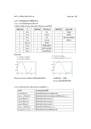
![บทที่ 3. การเขียนกราฟด้วย MATLABMATLAB – 42
ตัวอย่างเช่น
3.10.3 คําสั่งในการปรับค่าต่าง ๆ บนแกนพิกัด และการตีเส้นกริด
คําสั่ง ความหมายของคําสั่ง
grid on, grid off เขียนเส้นกริดหรือยกเลิกการเขียนเส้นกริด
axis on, axis off อนุญาต หรือไม่อนุญาต ให้กําหนดค่าต่าง ๆ เกี่ยวกับแกน
เช่น การตีเส้นกริด
axis square กําหนดให้กรอบในการเขียนกราฟเป็นสี่เหลี่ยมจัตุรัส
axis([xmin xmax ymin ymax])
กําหนดค่าสูงสุด และ ตํ่าสุดของแกน X และ แกน Y
axis([xmin xmax ymin ymax zmin zmax])
กําหนดค่าสูงสุด และ ตํ่าสุดของแกน X แกน Y และ แกน Z
ตัวอย่างเช่น](https://image.slidesharecdn.com/bookmathcadmathemeticamatlapmaple-160531122930/85/Book-mathcad-mathematica-matlap-maple-269-320.jpg)
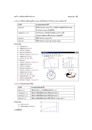
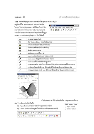
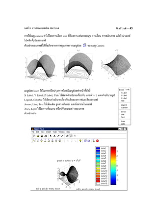
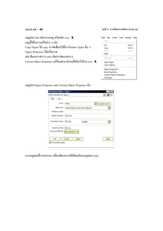
![บทที่ 4. การใช้งานเบื้องต้นเกี่ยวกับโปรแกรม MATLABMATLAB – 48
format rat
แสดงตัวเลขในลักษณะตัวเลขเศษส่วน
4.2 สัญลักษณ์พิเศษและ การกําหนดตัวแปรจํานวนใน MATLAB
เครื่องหมายหรือสัญลักษณ์ที่ใช้ในโปรแกรม MATLAB
เครื่องหมาย ความหมายและตัวอย่างการใช้งาน
( )
[ ]
subscripts
กําหนดข้อมูลเวกเตอร์ หรือ เมทริกซ์
=
;
↵
กําหนดค่า
รอการคํานวณ หรือใช้ในการคั่นคําสั่ง
สั่งคํานวณ
,
;
แยกสมาชิกในแถวของเมทริกซ์
แยกแถวของเมทริกซ์
% เป็นการทํา remark ของโปรแกรม
ตัวแปรจํานวนใน MATLAB จะเก็บข้อมูลตัวเลขในรูปแบบเมทริกซ์ คือจําแนกเป็นแถวและหลัก ตัวอย่างเช่น
การกําหนดค่า ความหมาย
กําหนดค่า 1 ค่าให้กับตัวแปร x
กําหนดค่าของตัวแปร x เป็นเมทริกซ์ 1 แถว 3 หลัก](https://image.slidesharecdn.com/bookmathcadmathemeticamatlapmaple-160531122930/85/Book-mathcad-mathematica-matlap-maple-275-320.jpg)
![บทที่ 4. การใช้งานเบื้องต้นเกี่ยวกับโปรแกรม MATLAB MATLAB – 49
กําหนดค่าของตัวแปร x เป็นเมทริกซ์ 1 แถว 3 หลัก
การเว้นช่องว่างหรือคั่นด้วย , มีผลเหมือนกัน
กําหนดค่าของตัวแปร x เป็นเมทริกซ์ 3 แถว 1 หลัก
การเว้นด้วย ; หมายถึงการขึ้นแถวใหม่
กําหนดค่าของตัวแปร x เป็นเมทริกซ์ 2 แถว 2 หลัก
การเว้นช่องว่าง แปลว่าอยู่แถวเดียวกัน
การเว้นด้วย ; หมายถึงการขึ้นแถวใหม่
การกําหนด x = a : d : b หมายถึง x มีค่าเป็นเวกเตอร์
x = [a, a + d, a+ 2d, ... ตัวสุดท้ายมีค่าไม่เกิน b]
4.3 การคํานวณเบื้องต้น
การคํานวณเกี่ยวกับตัวเลข และ ตัวแปรใน MATLAB มีหลายแบบดังนี้
การดําเนินงาน ตัวดําเนินการ ตัวอย่าง
การบวก +
การลบ –
การคูณ *
การคูณเชิงสมาชิก .*
การหารทางขวา /
a/b = b
a](https://image.slidesharecdn.com/bookmathcadmathemeticamatlapmaple-160531122930/85/Book-mathcad-mathematica-matlap-maple-276-320.jpg)
![บทที่ 4. การใช้งานเบื้องต้นเกี่ยวกับโปรแกรม MATLABMATLAB – 52
1. กําหนดค่า x = [1 2 3]
ใน Command Window
2. ใน Window Workspace
จะแสดงว่ามีการใช้ตัวแปร x ขนาด 1 × 3
3. ใน Command History
จะบันทึกคําสั่ง ที่สั่งไว้ใน Command Window
4.7 ฟังก์ชันทางคณิตศาสตร์และฟังก์ชันอื่น ๆ ที่สําคัญ
ฟังก์ชันทางคณิตศาสตร์
ฟังก์ชัน ความหมายและตัวอย่างการใช้งาน
abs(x) ค่าสัมบูรณ์ของ x หรือ ค่าสัมบูรณ์ของจํานวนเชิงซ้อน a + bi
angle(a + bi) ค่าอาร์กิวเมนต์ของจํานวนเชิงซ้อน a + bi
real(a + bi)
imag(a + bi)
ส่วนจริง และส่วนจินตภาพของจํานวนเชิงซ้อน
ceil(x) จํานวนเต็มที่เล็กที่สุดที่มีค่ามากกว่าหรือเท่ากับ x
conj(a + bi) ค่า conjugate ของตัวเลขเชิงซ้อน a + bi](https://image.slidesharecdn.com/bookmathcadmathemeticamatlapmaple-160531122930/85/Book-mathcad-mathematica-matlap-maple-279-320.jpg)
![บทที่ 4. การใช้งานเบื้องต้นเกี่ยวกับโปรแกรม MATLAB MATLAB – 55
eye(n)
eye(m, n)
eye(size(A))
เมทริกซ์เอกลักษณ์มิติ n × n
เมทริกซ์ m × n ที่สมาชิกในแนวทแยงมุมเป็น 1 นอกนั้นเป็น 0
เมทริกซ์ที่สมาชิกในแนวทแยงมุมเป็น 1 นอกนั้นเป็น 0 และมีมิติเหมือน
A
det(A), inv(A)
trace(A)
diag(A)
rank(A), poly(A)
ค่ากําหนดของเมทริกซ์ A, อินเวอร์สของเมทริกซ์ A
ผลบวกแนวทแยงมุมของเมทริกซ์ A
สมาชิกในแนวทแยงมุมของเมทริกซ์ A
ค่าลําดับชั้นของ A, พหุนามลักษณะเฉพาะของ A
eig(A)
[V, D] = eig(A)
eig(A) คือค่าเจาะจงของเมทริกซ์ A
V คือเวกเตอร์เจาะจงของเมทริกซ์ A
D คือเมทริกซ์ที่มีแนวทแยงมุมเป็นค่าเจาะจงของเมทริกซ์ A](https://image.slidesharecdn.com/bookmathcadmathemeticamatlapmaple-160531122930/85/Book-mathcad-mathematica-matlap-maple-282-320.jpg)
![บทที่ 4. การใช้งานเบื้องต้นเกี่ยวกับโปรแกรม MATLABMATLAB – 56
ฟังก์ชันเกี่ยวกับพหุนาม
หมายเหตุ p = [ na 1na − ... 1a 0a ] หมายถึงพหุนาม na
n
x + 1na −
1n
x
−
+ ... + 1a x + 0a
ฟังก์ชัน ความหมายและตัวอย่างการใช้งาน
1. polyder(p)
2. polyval(p, a)
3. [q, p]
= polyder(a, b)
1. อนุพันธ์ของพหุนาม p(x), 2. ค่าของฟังก์ชันพหุนาม p(a)
3. อนุพันธ์ของ )x(b
)x(a
มีค่าเป็น )x(p
)x(q
ตัวอย่างเช่น p(x) = 2 2
x + x + 4, p(3) = 25, p′(x) = 4x + 1
ความหมายคือ dx
d ( 1x
2xx2
−
++ ) =
1x2x
3x2x
2
2
+−
−−
conv(p, q) ผลคูณพหุนาม p(x)q(x) ตัวอย่างเช่น p(x) = x + 2, q(x) = 3x + 4,
p(x)q(x) = 3 2
x + 10x + 8
deconv(p, q) ผลลัพธ์ของการหารพหุนาม p(x) ด้วย q(x)
ความหมายคือ
2x3x
5x51x
2x3x
3x4x2x
22
23
++
++−=
++
+++
roots(p)
fzero(f, a)
roots(p) = รากของพหุนาม p(x) = 0
fzero(f, x) = รากของ f(x) = 0 โดยมีค่าเริ่มต้นที่ a](https://image.slidesharecdn.com/bookmathcadmathemeticamatlapmaple-160531122930/85/Book-mathcad-mathematica-matlap-maple-283-320.jpg)
![บทที่ 4. การใช้งานเบื้องต้นเกี่ยวกับโปรแกรม MATLAB MATLAB – 57
poly(v)
poly(A)
พหุนาม p(x) ที่มีรากเป็นสมาชิกของเวกเตอร์ v
พหุนามลักษณะเฉพาะของเมทริกซ์ A
คําสั่งเกี่ยวกับการจัดรูปแบบพีชคณิตของฟังก์ชัน
ฟังก์ชัน ความหมายและตัวอย่างการใช้งาน
expand(f)
factor(f)
collect(f)
simplify(f)
กระจายสูตร
แยกตัวประกอบ
กระจายสูตร
จัดรูปแบบพีชคณิตให้มีรูปแบบอย่างง่าย
pretty(f)
poly2sym(p)
sym2poly(p)
แสดงสูตรของพหุนาม
เปลี่ยนเวกเตอร์ของสัมประสิทธิ์เป็นพหุนาม
เปลี่ยนพหุนามเป็นเวกเตอร์สัมประสิทธิ์
[a, b, k]
= residue(p, q)
การแยกเศษส่วนพหุนาม )x(q
)x(p
เป็นเศษส่วนย่อย](https://image.slidesharecdn.com/bookmathcadmathemeticamatlapmaple-160531122930/85/Book-mathcad-mathematica-matlap-maple-284-320.jpg)
![บทที่ 4. การใช้งานเบื้องต้นเกี่ยวกับโปรแกรม MATLABMATLAB – 58
ความหมายคือ
x
1 + 1x
2
−
+ 1x
3
+
+ 2x + 3 =
xx
1x4x4x3x2
3
234
−
−−++
[p, q]
= residue(a, b, k)
จัดรูปผลบวกของเศษส่วนย่อยเป็น )x(q
)x(p
xx
1x4x4x3x2
3
234
−
−−++ = x
1 + 1x
2
−
+ 1x
3
+
+ 2x + 3
โดยการคํานวณของ MATLAb
คําสั่งเกี่ยวกับแคลคูลัส
ฟังก์ชัน ความหมายและตัวอย่างการใช้งาน
sum(x)
symsum(f(n))
symsum(f(n),a,b)
ผลบวกสมาชิกใน x
หาผลรวม f(n) จาก 1 ถึง n, หาผลรวม f(n) จาก a ถึง b
limit(f)
limit(f, a)
limit(f, h, a)
limit(f, n, inf)
limit(f,x,a,'left')
limit(f,x,a,'right')
)x(flim
0x→
, )x(flim
ax→
, )h,x(flim
ah→
, )n(flim
n ∞→
, )x(flim
ax −→
,
)x(flim
ax +→
ตามลําดับ](https://image.slidesharecdn.com/bookmathcadmathemeticamatlapmaple-160531122930/85/Book-mathcad-mathematica-matlap-maple-285-320.jpg)
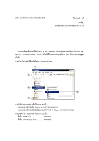
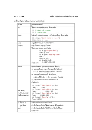
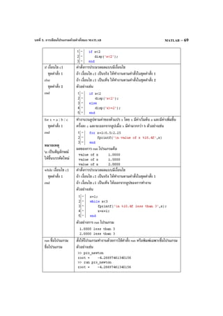
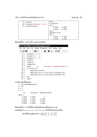
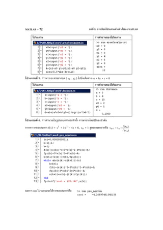
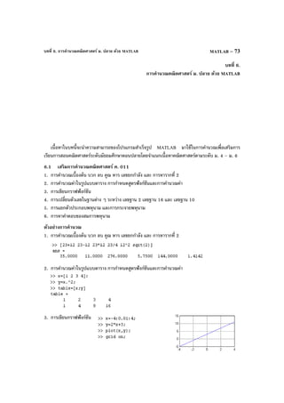
![บทที่ 6. การคํานวณคณิตศาสตร์ ม. ปลาย ด้วย MATLABMATLAB – 74
4. การเปลี่ยนตัวเลขในฐานต่าง ๆ ระหว่าง เลขฐาน 2 เลขฐาน 16 และ เลขฐาน 10
5. การแยกตัวประกอบ และ การกระจายพหุนาม
6. การหารากของสมการพหุนาม เช่นการหารากของ 2
x – 3x – 4 = 0
หมายเหตุ [1 –3 –4] หมายถึง พหุนาม 2
x – 3x – 4
roots([1 –3 –4]) เป็นคําสั่งหารากของพหุนาม
2
x – 3x – 4 = 0
6.2 เสริมการคํานวณคณิตศาสตร์ ค. 012
1. การเขียนกราฟ วงกลม พาราโบลา วงรี ไฮเพอร์โบลา
2. การคํานวณค่าฟังก์ชันตรีโกณมิติ sin, cos, tan, sec, cosec, cot
3. กราฟของ sin, cos, tan, sec, cosec, cot
4. การหาค่าเฉลี่ยเลขคณิต
ตัวอย่างการคํานวณ
1. การเขียนกราฟ วงกลม พาราโบลา วงรี ไฮเพอร์โบลา
การเขียนกราฟของวงกลม 2
x + (y + 3)2
= 16
การเขียนกราฟของพาราโบลา y = 2
x
8
1](https://image.slidesharecdn.com/bookmathcadmathemeticamatlapmaple-160531122930/85/Book-mathcad-mathematica-matlap-maple-301-320.jpg)
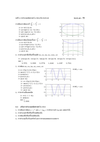
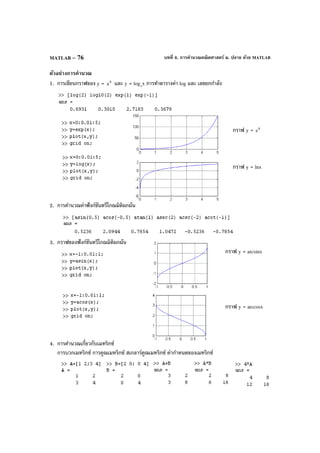
![บทที่ 6. การคํานวณคณิตศาสตร์ ม. ปลาย ด้วย MATLAB MATLAB – 79
ตัวอย่างการคํานวณ
1. การคํานวณ n!, r
n
P , r
n
C และ การกระจายทวินาม
2. กราฟแผนภาพการกระจายของข้อมูล
3. การวิเคราะห์ความสัมพันธ์เชิงฟังก์ชันระหว่างข้อมูล
สมการแสดงความสัมพันธ์ของข้อมูลคือ y = 3.3x – 1.7
6.7 MATLAB กับการเฉลยข้อสอบคณิตศาสตร์ Entrance
ในหัวข้อนี้จะเป็นการนําความสามารถของ MATLAB เข้ามาช่วยหาคําตอบของข้อสอบ ซึ่งมีข้อสอบ Entrance
หลายข้อที่เราหาคําตอบได้ด้วยการแทนค่า คํานวณค่า หรือแม้แต่เขียนกราฟดูก็จะได้คําตอบ
ข้อสอบคณิตศาสตร์ 1. มีนาคม 2546 ข้อ 18.
0x
lim
→ 3
x
1 [ x1+ – x1− – )x1)(x1( 2
−+ + )x1)(x1( 2
−− ] มีค่าเท่ากับข้อใดต่อไปนี้
1. 0 2. 4
1
3. 2
1 4. 1](https://image.slidesharecdn.com/bookmathcadmathemeticamatlapmaple-160531122930/85/Book-mathcad-mathematica-matlap-maple-306-320.jpg)
![บทที่ 7. เสริมการคํานวณระดับอุดมศึกษาด้วย MATLABMATLAB – 82
7.1.4 กราฟของฟังก์ชัน f, f′ และ f′′
7.1.5 การหาผลบวกรีมันน์ (Riemann sum)
เช่นผลบวกรีมันน์ของ f(x) = 2
x – 4x + 6 บนช่วง [1, 3]
ค่าของ dx)6x4x(
2
3
1
+−∫ = 4.666666
7.1.6 การแทนฟังก์ชันด้วยพหุนามเทย์เลอร์ เช่น พหุนามเทย์เลอร์ของ sin(x), arctan(x), cos(x), x
e
7.1.7 การเขียนกราฟในพิกัดเชิงขั้ว
ตัวอย่างเช่นกราฟของ r = 4cos(2t)](https://image.slidesharecdn.com/bookmathcadmathemeticamatlapmaple-160531122930/85/Book-mathcad-mathematica-matlap-maple-309-320.jpg)
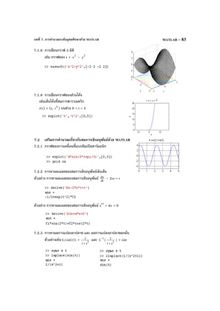
![บทที่ 7. เสริมการคํานวณระดับอุดมศึกษาด้วย MATLABMATLAB – 84
7.3 เสริมการคํานวณเกี่ยวกับการวิเคราะห์เชิงตัวเลขด้วย MATLAB
7.3.1 การประมาณเส้นโค้ง y(x) ที่ผ่านจุด ( 1x , 1y ), ( 2x , 2y ), ... , ( nx , ny )
จงหาสมการเส้นโค้ง y(x) ที่ผ่านจุด (3, 4), (6, 13), (8, 6), (11, 10), (15, 13) และ (17, 18)
7.3.2 การประมาณค่าภายในช่วงจากข้อมูล ( 1x , 1y ), ( 2x , 2y ), ... , ( nx , ny )
ตัวอย่างข้อมูล
โดยวิธี linear interpolation y(10) = 15.7
โดยวิธี spline interpolation y(10) = 15.9301
7.3.3 การหารากของสมการ ตัวอย่าง การหารากของสมการ 2
x – 5 = 0
p = [1 0 –5] หมายถึงพหุนาม 2
x – 5
roots(p) เป็นคําสั่งหารากของ p(x) = 0
ราก 2
x – 5 = 0 คือ x = 2.2361, –2.361
การหารากของสมการ sinx – cosx = 0
เพราะฉะนั้นรากสมการ sinx – cosx = 0 คือ 4
π
7.3.4 การหาผลเฉลยของระบบสมการเชิงเส้น และ ไม่เชิงเส้น
ตัวอย่าง การหาผลเฉลยของระบบสมการ x + y + z = 12
x – y + z = 4
x + y – z = 2
x y
2 3
5 5
7 9
11 18
15 22](https://image.slidesharecdn.com/bookmathcadmathemeticamatlapmaple-160531122930/85/Book-mathcad-mathematica-matlap-maple-311-320.jpg)
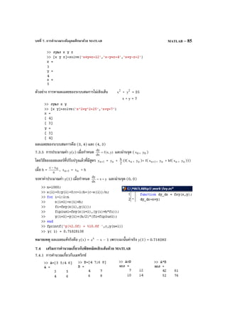
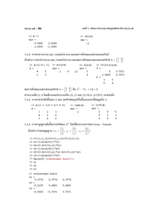
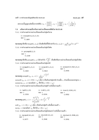
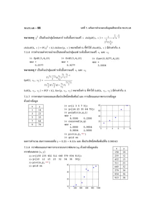
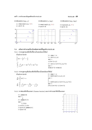
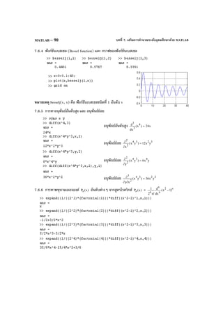
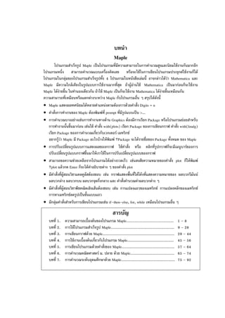
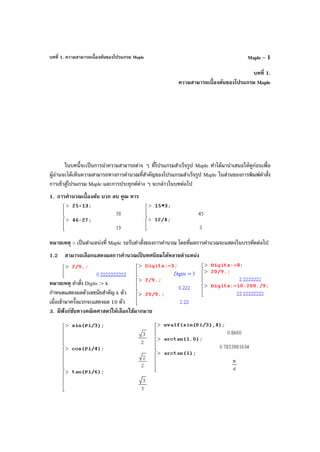
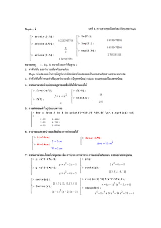
![บทที่ 1. ความสามารถเบื้องต้นของโปรแกรม Maple Maple – 3
หมายเหตุ roots(r) = [[1, 3], [2, 1], [3, 1]]
หมายถึงพหุนาม r(x) = 0 มีราก 1 ซํ้า 3 ตัว ราก 2 ซํ้า 1 ตัว ราก 3 ซํ้า 1 ตัว
8. ความสามารถในการเขียนกราฟได้หลายแบบ
8.1 กราฟในระบบพิกัดมุมฉาก
ตัวอย่าง กราฟของ f(x) = 2x + 3 บนช่วง [–5, 5]
8.2 สามารถเขียนกราฟได้หลายเส้นพร้อมกัน
ตัวอย่าง กราฟของ f(x) = 2x + 3 กับ g(x) = 2
x – 4 บนช่วง [–5, 5]
8.3 สามารถเขียนกราฟแบบคู่ลําดับ
ตัวอย่าง กราฟของข้อมูล นํ้าหนักและส่วนสูง
นํ้าหนัก ความสูง
53 156
58 165
55 162
60 170
62 165
68 173](https://image.slidesharecdn.com/bookmathcadmathemeticamatlapmaple-160531122930/85/Book-mathcad-mathematica-matlap-maple-322-320.jpg)
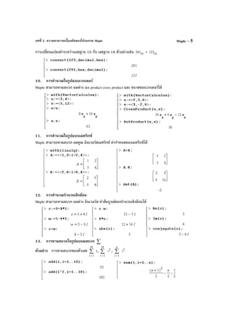
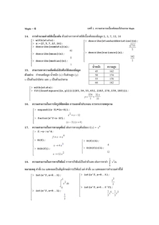
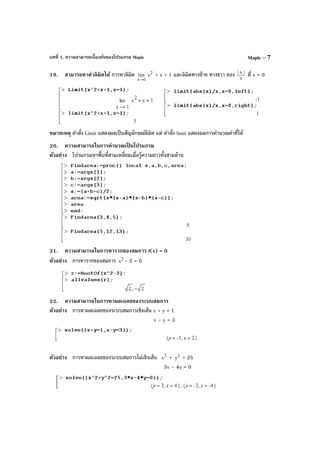
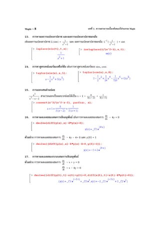
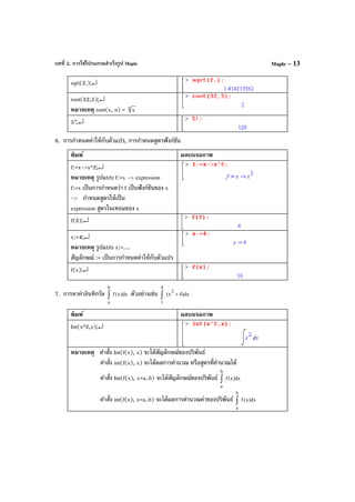
![บทที่ 2. การใช้โปรแกรมสําเร็จรูป MapleMaple – 14
Int(x^2,x);↵
Int(x^2,x=0..1);↵
int(x^2,x=0..1);↵
2.3 การเขียนกราฟของฟังก์ชัน
ตัวอย่างเช่นการเขียนกราฟของ f(x) = 2
x – 3x – 7 บนช่วง [–8, 8]
พิมพ์ ผลบนจอภาพ
plot(x^2-3*x-7,x=-8..8);↵
หมายเหตุ plot(f(x), x = a .. b)
เป็นคําสั่งเขียนกราฟ y = f(x) บน
ช่วง [a, b]
2.4 การกําหนดค่าและการคํานวณเกี่ยวกับเมทริกซ์
ตัวอย่าง การกําหนด A =
−
−
35
24 และ B =
31
52
พิมพ์ ผลบนจอภาพ
with(linalg):↵
หมายเหตุ with(linalg) เป็นคําสั่งเรียกโปรแกรมคํานวณ
เกี่ยวกับเมทริกซ์ของ Maple มาใช้งาน
คําสั่งกําหนดเมทริกซ์ A = nmij]a[ × คือ
A:=<< 11a , 21a , ... , 1ma >|< 12a , 22a , ... , 2ma >| ... |< n1a , n2a , ... , mna >>
A:=<<4,-5>|<-2,3>>;↵
B:=<<2,1>|<5,3>>;↵](https://image.slidesharecdn.com/bookmathcadmathemeticamatlapmaple-160531122930/85/Book-mathcad-mathematica-matlap-maple-333-320.jpg)
![บทที่ 2. การใช้โปรแกรมสําเร็จรูป Maple Maple – 15
การคํานวณค่าของเมทริกซ์ A + B, AB, 4A, 2
A , 1
A
−
, T
A , det(A)
พิมพ์ ผลบนจอภาพ
A+B;↵
A.B;↵
หมายเหตุ สัญลักษณ์ (.) จุดแทน
การคูณเมทริกซ์กับเมทริกซ์
4*A;↵
A^2;↵
A^(–1);↵
หมายเหตุ inverse(A) ใช้หา 1
A
−
ได้เหมือนกับ A^(–1)
det(A)↵
transpose(A);↵
การกําหนดดรรชนีล่าง (subscript) สําหรับอ้างอิงใช้งานกับสมาชิกของเมทริกซ์
พิมพ์ ผลบนจอภาพ
A[1,1];↵
หมายเหตุ A[i, j] คือ ija ของเมทริกซ์ A = nmij]a[ ×
การอ้างอิง แถว และ หลักของเมทริกซ์
พิมพ์ ผลบนจอภาพ
with(LinearAlgbra);↵
A:=<<4,-5>|<-2,3>>;↵](https://image.slidesharecdn.com/bookmathcadmathemeticamatlapmaple-160531122930/85/Book-mathcad-mathematica-matlap-maple-334-320.jpg)
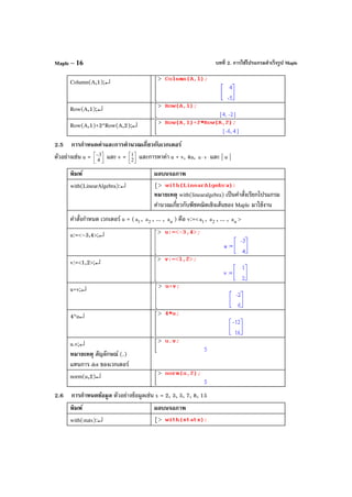
![บทที่ 2. การใช้โปรแกรมสําเร็จรูป Maple Maple – 17
หมายเหตุ with(stats) เป็นคําสั่งเรียกโปรแกรมคํานวณ
เกี่ยวกับสถิติของ Maple มาใช้งาน
x:=[2,3,5,7,8,15];↵
x[2];↵
หมายเหตุ ข้อมูลตัวที่ i แทนด้วย x[i]
describe[range](x);↵
คําสั่งแสดงค่า ตํ่าสุด .. สูงสุดของข้อมูล
describe[mean](x);↵
describe[median](x);↵
describe[variance](x);↵
describe
[standarddeviation](x);↵
ใน Maple มีฟังก์ชันที่ช่วยคํานวณค่าทางด้านสถิติของข้อมูลดังนี้
describe[mean](x) = ค่าเฉลี่ยเลขคณิตของข้อมูล describe[median](x) = มัธยฐานของข้อมูล
describe[variance](x) = ความแปรปรวนของข้อมูล(ประชากร)
describe[standarddeviation](x) = ส่วนเบี่ยงเบนมาตรฐานของข้อมูล(ประชากร)
describe[range](x) = แสดงค่า ตํ่าสุด ... สูงสุด ของข้อมูล
2.7 การกําหนดข้อมูล 2 ตัวแปรและการเขียนแผนภาพการกระจาย
ตัวอย่างข้อมูล
พิมพ์ ผลบนจอภาพ
with(stats):↵
x:=[3,5,9,12];↵
y:=[12,15,21,32];↵
x y
3 12
5 15
9 21
12 32](https://image.slidesharecdn.com/bookmathcadmathemeticamatlapmaple-160531122930/85/Book-mathcad-mathematica-matlap-maple-336-320.jpg)
;↵
2.8 การคํานวณค่าเกี่ยวกับผลบวกในรูปแบบ ∑ ตัวอย่างเช่น การหาค่าของ ∑
=
10
1i
i , ∑
=
10
1i
2
i , ∑
=
n
1i
i
พิมพ์ ผลบนจอภาพ
add(i,i=1..10);↵
คําสั่ง add( ix ,i=a..b) เป็นการหาผลบวก i
b
ai
x∑
=
sum( ix ,i=a..b) เป็นการหาผลบวก i
b
ai
x∑
=
ได้เป็นผลการคํานวณ หรือ เป็นสูตร
Sum( ix ,i=a..b) เป็นคําสั่งแสดงผลในรูปแบบสัญลักษณ์ผลบวก
add(i^2,i=1..10);↵
sum(i,i=1..10);↵
sum(i,i=1..n);↵
Sum(i,i=1..n);↵
2.9 การคํานวณค่าปริพันธ์จํากัดเขตและปริพันธ์ไม่จํากัดเขต และปริพันธ์ 2 ตัวแปร
ตัวอย่างเช่น การหาค่าของ dxx
2
1
0
∫ , dxx
2
2
t
t
∫ , dxdx)yx(
2
∫∫ และ dxdy)yx(
2
2
1
3
0
∫∫
พิมพ์ ผลบนจอภาพ
int(x^2,x=0..1);↵](https://image.slidesharecdn.com/bookmathcadmathemeticamatlapmaple-160531122930/85/Book-mathcad-mathematica-matlap-maple-337-320.jpg)
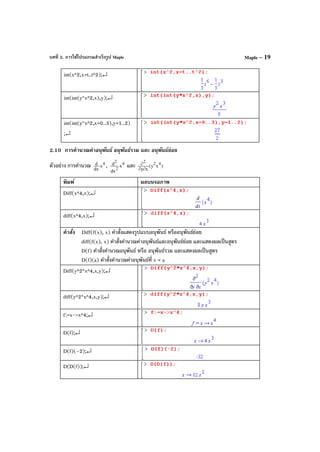
![บทที่ 2. การใช้โปรแกรมสําเร็จรูป Maple Maple – 21
convert(18,binary);↵
convert(18,base,2);↵
convert(“12”,decimal,hex);↵
convert(“10010”,decimal,
2);↵
convert(“10010”,decimal,
binary);↵
convert(“22”,decimal,octal);↵
2.13 การหาผลบวกในรูปแบบ ∑
=
n
1i
ix
ตัวอย่าง การหาค่าของ ∑
=
4
1i
ix , ∑
=
4
1i
iy , ∑
=
4
1i
2
ix , ∑
=
4
1i
2
iy , ∑
=
4
1i
iiyx จากข้อมูล
พิมพ์ ผลบนจอภาพ
x:=[2,3,6,9];↵
y:=[12,15,14,19];↵
sum(x[i],i=1..4);↵
sum(y[i],i=1..4);↵
sum(x[i]^2,i=1..4);↵
sum(y[i]^2,i=1..4);↵
sum(x[i]*y[i],i=1..4);↵
2.14 การสร้างตารางฟังก์ชัน
การคํานวณค่า f(x) = 2 2
x + 4, x = 2, 3, 5 ในรูปแบบตาราง
พิมพ์ ผลบนจอภาพ
x:=[2,3,5]:↵
x y
2 12
3 15
6 14
9 19](https://image.slidesharecdn.com/bookmathcadmathemeticamatlapmaple-160531122930/85/Book-mathcad-mathematica-matlap-maple-340-320.jpg)
![บทที่ 2. การใช้โปรแกรมสําเร็จรูป MapleMaple – 22
f:=x->2*x^2+4;↵
พิมพ์
for i from 1 to 3 do;↵ บรรทัดแรกของโปรแกรม เริ่มคําสั่ง for
printf(“%10.1f %20.2f”,x[i],f(x[i]));↵ บรรทัดที่ 2 ของโปรแกรม
od;↵ บรรทัดที่ 3 ของโปรแกรม จบคําสั่ง for
ผลบนจอภาพ
คําอธิบายเพิ่มเติม for i from a to b do
ชุดคําสั่ง
od
เป็นชุดคําสั่งของการทํางานเป็นลูบ โดยตัวแปร i เปลี่ยนค่าจาก a ถึง b
printf คือคําสั่งพิมพ์ โดยมีรูปแบบกําหนดการพิมพ์ตัวเลขเช่น
รูปแบบ %10.1f หมายถึงเตรียมช่องว่าง 10 ที่แล้วพิมพ์เลขทศนิยม 1 ตําแหน่ง
%n.kf หมายถึงเตรียมช่องว่าง n ที่แล้วพิมพ์เลขทศนิยม k ตําแหน่ง
n เป็นคําสั่งขึ้นบรรทัดใหม่ก่อนพิมพ์
2.15 การคํานวณค่าเกี่ยวกับจํานวนเชิงซ้อน
ตัวอย่าง z = 3 + 4i, w = 5 – 9i การหาค่า z + w, zw, | z |, อาร์กิวเมนต์ของ z, Re(z), Im(z) และ z
พิมพ์ ผลบนจอภาพ
z:=3+4*I:↵
หมายเหตุ I = 1−
w:=5–9*I;↵
z+w;↵
4*z;↵
z.w;↵
หมายเหตุ . แทนการคูณของ
จํานวนเชิงซ้อนกับจํานวนเชิงซ้อน](https://image.slidesharecdn.com/bookmathcadmathemeticamatlapmaple-160531122930/85/Book-mathcad-mathematica-matlap-maple-341-320.jpg)
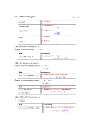
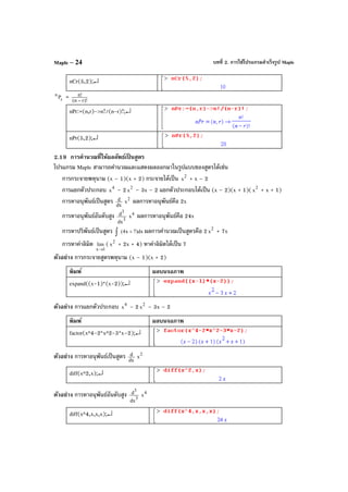
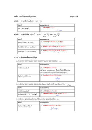
![บทที่ 2. การใช้โปรแกรมสําเร็จรูป MapleMaple – 26
series(sin(x),x,5);↵
taylor(sin(x),x,8);↵
2.20.4 การแยกเศษส่วนย่อยด้วยโปรแกรม Maple
2xx
x
2
3
−−
สามารถแยกเป็นผลบวกย่อย x + 1 + )2x(3
8
−
+ )1x(3
1
+
ด้วยคําสั่ง convert
พิมพ์ convert(x^3/(x^2-x-2),parfrac,x);↵
ผลบนจอภาพ
การกระจาย x + 1 + )2x(3
8
−
+ )1x(3
1
+
เป็น )2x)(1x(
x3
−+
ได้ด้วยคําสั่ง factor
พิมพ์ factor(x+1+8/(3*(x-2))+1/(3*(x+1)));↵
ผลบนจอภาพ
2.20.5 การหาผลเฉลยของสมการเชิงอนุพันธ์ ตัวอย่าง การหาผลเฉลยของสมการ dx
dy
– 4y = 0
พิมพ์ dsolve(diff(y(x),x)-4*y(x)=0);↵
ผลบนจอภาพ
หมายเหตุ คําสั่ง dsolve(สมการ), dsolve([สมการ 1, สมการ 2, ...]) , dsolve({สมการ 1, สมการ 2, ...})
เป็นคําสั่งช่วยในการหาผลเฉลยของสมการเชิงอนุพันธ์และผลเฉลยของระบบสมการเชิงอนุพันธ์
โดยมี diff(y[x], x) = dt
dy
, diff(y[x], x, x) = 2
2
dx
yd
และ diff(y[x], x$k) หมายถึงอนุพันธ์ k
k
dx
yd
การคํานวณแบบที่ 2. คือ](https://image.slidesharecdn.com/bookmathcadmathemeticamatlapmaple-160531122930/85/Book-mathcad-mathematica-matlap-maple-345-320.jpg)
![บทที่ 2. การใช้โปรแกรมสําเร็จรูป Maple Maple – 27
ตัวอย่าง การหาผลเฉลยของสมการเชิงอนุพันธ์ dx
dy
– 4y = 4
พิมพ์ dsolve(diff(y(x),x)-4*y(x) = 4);↵
ผลบนจอภาพ
แบบที่ 2.
ตัวอย่าง การหาผลเฉลยของสมการเชิงอนุพันธ์ dx
dy
– 4y = 4 และ y(0) = 1
พิมพ์ dsolve([diff(y(x),x)-4*y(x))=4,y(0)=1]);↵
ผลบนจอภาพ
แบบที่ 2.
ตัวอย่าง การหาผลเฉลยของสมการเชิงอนุพันธ์ 2
2
dx
yd
+ 4y = 0
พิมพ์ dsolve(diff(y(x),x,x)+4*y(x)=0);↵
ผลบนจอภาพ
แบบที่ 2.
2.20.6 การหาผลเฉลยของระบบสมการเชิงอนุพันธ์
ตัวอย่าง การหาผลเฉลยของระบบสมการเชิงอนุพันธ์ dt
dy
– x + y = 0
dt
dx + x – 4y = 0
พิมพ์ dsolve([diff(y(t),t)-x(t)+y(t)=0,diff(x(t),t)-x(t)+y(t)=0]);↵](https://image.slidesharecdn.com/bookmathcadmathemeticamatlapmaple-160531122930/85/Book-mathcad-mathematica-matlap-maple-346-320.jpg)
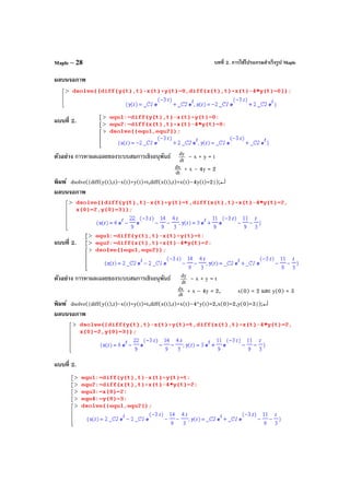
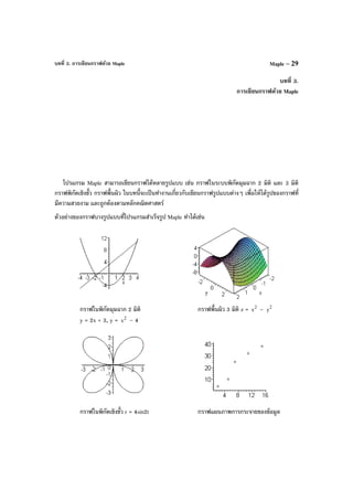
![บทที่ 3. การเขียนกราฟด้วย MapleMaple – 30
3.1 การเขียนกราฟในระบบพิกัดมุมฉาก 2 มิติ
ตัวอย่าง การเขียนกราฟของ y = 2x + 3 บนช่วง [–4, 4] โดยใช้คําสั่ง plot
พิมพ์ ผลบนจอภาพ
plot(2*x+3,x=-4..4);↵
หมายเหตุ plot(f(x), x = a .. b) เป็นคําสั่งเขียนกราฟ y = f(x) บนช่วง [a, b]
ตัวอย่าง การเขียนกราฟของ y = 2x + 3 และ y = 2
x – 4 บนช่วง [–4, 4]
พิมพ์ ผลบนจอภาพ
plot({2*x+3,x^2–4}, x=-
4..4);↵
หมายเหตุ plot({f(x), g(x)}, x = a .. b) เป็นคําสั่งเขียนกราฟ y = f(x) และ y = g(x) บนช่วง [a, b]
การเขียนกราฟโดยกําหนดสูตรฟังก์ชันไว้ก่อนทําได้ดังนี้
3.2 การเขียนกราฟแจกแจงความถี่ กราฟแท่ง
ตัวอย่างข้อมูลเช่น
ช่วงคะแนน ความถี่
0 – 1.0 15
1.1 – 2.0 35
2.1 – 3.0 40
3.1 – 4.0 10](https://image.slidesharecdn.com/bookmathcadmathemeticamatlapmaple-160531122930/85/Book-mathcad-mathematica-matlap-maple-349-320.jpg)
![บทที่ 3. การเขียนกราฟด้วย Maple Maple – 31
พิมพ์ with(stats):↵
ผลบนจอภาพ
(หมายเหตุ เรียกโปรแกรมทํางานทางด้านสถิติขึ้นมาใช้งาน)
พิมพ์ data:=[Weight(0..1.0,15),Weight(1.1..2.0,35),
Weight(2.1..3.0,40),Weight(3.1..4.0,10)];↵
ผลบนจอภาพ
พิมพ์ statplots[histogram](data);↵
ผลบนจอภาพ
หมายเหตุ with(stats): เป็นคําสั่งเรียกโปรแกรมทํางานทางด้านสถิติขึ้นมาใช้งาน
Weight(a .. b, f) เป็นคําสั่งกําหนดความถี่ของช่วงคะแนน (a – b)
statplots[histogram](data) เป็นคําสั่งเขียนกราฟแจกแจงความถี่ของข้อมูล
ตัวอย่างการเขียนกราฟ histogram ของข้อมูล 1, 4, 1, 1,2. 2, 3, 2 , 2 และ 3
(1) เรียก package stats (2) กําหนดข้อมูล (3) กําหนดช่วงคะแนนที่ใช้ในการแจกแจงความถี่
(4) ทําการแจกแจงความถี่ของข้อมูล data ด้วยช่วงคะแนน interval โดยใช้คําสั่ง transform (5) เขียนกราฟ](https://image.slidesharecdn.com/bookmathcadmathemeticamatlapmaple-160531122930/85/Book-mathcad-mathematica-matlap-maple-350-320.jpg)
![บทที่ 3. การเขียนกราฟด้วย MapleMaple – 32
3.3 การเขียนกราฟของแผนภาพการกระจายของข้อมูล
ตัวอย่างของข้อมูลเช่น
พิมพ์ ผลบนจอภาพ
with(stats):↵
x:=[53,58,55,60,62,68];↵
y:=[156,165,162,170,165,
173];↵
statplots[scatterplot](x,y);↵
3.4 การเขียนกราฟในระบบพิกัดเชิงขั้ว ตัวอย่าง การเขียนกราฟ r = 4sin(2t)
พิมพ์ plot(4*sin(2*t),t=0..2*Pi,coords=polar);↵
ผลบนจอภาพ
ตัวอย่าง การเขียนกราฟ โดยกําหนดสูตรฟังก์ชันก่อน และการเขียนกราฟ 2 เส้นบนสเกลเดียวกัน
x y
53 156
58 165
55 162
60 170
62 165
68 173](https://image.slidesharecdn.com/bookmathcadmathemeticamatlapmaple-160531122930/85/Book-mathcad-mathematica-matlap-maple-351-320.jpg)
![บทที่ 3. การเขียนกราฟด้วย Maple Maple – 33
3.5 การเขียนกราฟของสมการพาราเมตริก
3.5.1 กราฟพาราเมตริก 2 มิติ ตัวอย่างเช่น การเขียนกราฟของเส้นโค้งที่มีสมการพาราเมตริก
x(t) = 80t และ y(t) = –16 2
t + 80t บนช่วง 0 < t < 5
พิมพ์ plot([80*t,-16*t^2+80*t,t=0..5]);↵
ผลบนจอภาพ
3.5.2 กราฟพาราเมตริก 3 มิติ
ตัวอย่างเช่น กราฟของสมการพาราเมตริก x(t) = cost, y(t) = sint และ z(t) = 4
t บนช่วง 0 < t < 2π
พิมพ์ ผลบนจอภาพ
with(plots):↵
x:=t->2*sin(t);↵
y:=t->2*cos(t);↵
z:=t->t/4;↵
พิมพ์ spacecurve([x(t),y(t),z(t)],t=0..4*Pi,axes=BOXED,colour=black);↵
ผลบนจอภาพ](https://image.slidesharecdn.com/bookmathcadmathemeticamatlapmaple-160531122930/85/Book-mathcad-mathematica-matlap-maple-352-320.jpg)
![บทที่ 3. การเขียนกราฟด้วย MapleMaple – 34
หมายเหตุ spacecurve เป็นคําสั่งเขียนกราฟใน 3 มิติ
colour = ... เป็นคําสั่งกําหนดสีของกราฟ
axes = BOXED เป็นคําสั่งกําหนดให้แสดงกรอบของสเกลแกน XYX
3.6 การเขียนกราฟพื้นผิว 3 มิติ และกราฟแบบ contour
ตัวอย่าง การเขียนกราฟพื้นผิว f(x, y) = 2
x – 2
y บนช่วง [–2, 2] × [–2, 2] และกราฟ contour
พิมพ์ ผลบนจอภาพ
with(plots):↵
พิมพ์ plot3d(x^2-y^2,x=-2..2,y=-3..3,axes=BOXED);↵
ผลบนจอภาพ
พิมพ์ contourplot3d(x^2-y^2,x=-2..2,y=-3..3,axes=BOXED,style=CONTOUR,
orientation=[90,0],colour=black);↵
ผลบนจอภาพ
หมายเหตุ contourplot3d เป็นคําสั่งเขียนกราฟ contour
style = .... เป็นคําสั่งกําหนดรูปแบบการ plot
orientation = .... เป็นคําสั่งกําหนดมุมมอง ของกราฟที่ได้
คําแนะนํา ในกรณีที่คําสั่งและเงื่อนไขมีข้อความมาก ควรขึ้นบรรทัดใหม่ด้วยการกด <Shift>+↵](https://image.slidesharecdn.com/bookmathcadmathemeticamatlapmaple-160531122930/85/Book-mathcad-mathematica-matlap-maple-353-320.jpg)
![บทที่ 3. การเขียนกราฟด้วย Maple Maple – 35
3.7 การเขียนกราฟของความสัมพันธ์ ตัวอย่าง การเขียนของวงรี 25
x2
+ 16
y2
= 1
พิมพ์ ผลบนจอภาพ
with(plots):↵
พิมพ์ implicitplot(x^2/25+y^2/16=1,x=-5..5,y=-4..4,scaling=CONSTRAINED);↵
ผลบนจอภาพ
หมายเหตุ implicitplot เป็นคําสั่งเขียนกราฟของความสัมพันธ์
3.8 การเขียนกราฟสนามเวกเตอร์
ตัวอย่าง การเขียนกราฟฟังก์ชันค่าเวกเตอร์ F(x, y) = (x + y, x – y) บนช่วง [-1, 1] × [–2, 2]
พิมพ์ ผลบนจอภาพ
with(plots):↵
พิมพ์ fieldplot([x+y,x-y],x=-1..1,y=-2..2);↵
ผลบนจอภาพ
ตัวอย่าง การเขียนกราฟฟังก์ชัน F(x, y, z) = (x + y, x – y, z) บนช่วง [0, 1] × [0, 2] × [0, 1]
พิมพ์ ผลบนจอภาพ
with(plots):↵
พิมพ์
fieldplot3d([x+y,x-y,z],x=0..1,y=0..2,z=0..1,axes=FRAMED,colour=black);↵](https://image.slidesharecdn.com/bookmathcadmathemeticamatlapmaple-160531122930/85/Book-mathcad-mathematica-matlap-maple-354-320.jpg)
![บทที่ 3. การเขียนกราฟด้วย MapleMaple – 36
ผลบนจอภาพ
หมายเหตุ fieldplot, fieldplot3d เป็นคําสั่งเขียนกราฟของสนามเวกเตอร์
3.9 การเขียนกราฟของ gradient vector
ตัวอย่าง การเขียนกราฟ gradient ของฟังก์ชัน f(x, y) = 2
x y บนช่วง [-2, 2] × [–1, 1]
และการเขียนกราฟ gradient ของฟังก์ชัน f(x, y, z) = 2
x + yz บนช่วง [0, 1] × [0, 1] × [0, 1]
พิมพ์ ผลบนจอภาพ
with(plots):↵
พิมพ์ gradplot(x^2*y,x=-2..2,y=-1..1);↵
ผลบนจอภาพ
พิมพ์ gradplot3d(x^2+y*z,x=0..1,y=0..1,z=0..1,axes=FRAMED,colour=black);↵
ผลบนจอภาพ
หมายเหตุ gradplot, gradplot3d เป็นคําสั่งเขียนกราฟของ graddient vector field](https://image.slidesharecdn.com/bookmathcadmathemeticamatlapmaple-160531122930/85/Book-mathcad-mathematica-matlap-maple-355-320.jpg)
![บทที่ 3. การเขียนกราฟด้วย Maple Maple – 37
3.10 การปรับรูปแบบกราฟให้สวยงาม
โปรแกรม Maple มีคําสั่งในการปรับรูปแบบของการเขียนกราฟได้หลายลักษณะ โดยมีคําสั่งที่สําคัญและนิยม
ใช้งานดังต่อไปนี้
คําสั่ง หน้าที่และตัวอย่างการใช้งาน
colour กําหนดสีของเส้นกราฟ เช่น colour = black, colour = red
thichness กําหนดความหนาของเส้นกราฟ เช่น thickness = 1, 2 , 3, ...
style
symbol
numpoints
symbolsize
style กําหนดรูปแบบการเขียนกราฟแบบ line, point, patch, patchnogrid
symbol กําหนดสัญลักษณ์การ plot จุดเช่น box([]). circle(o)
numpoints กําหนดจํานวนจุดในการ plot
symbolsize กําหนดขนาดของ symbol ในการเขียนกราฟ](https://image.slidesharecdn.com/bookmathcadmathemeticamatlapmaple-160531122930/85/Book-mathcad-mathematica-matlap-maple-356-320.jpg)
![บทที่ 3. การเขียนกราฟด้วย MapleMaple – 38
linestyle กําหนดรูปแบบของเส้น เช่น linestyle = SOLID, DOT, DASH, DASHDOT
filled กําหนดการแรเงาระหว่างเส้นโค้งกับแกน X
axes กําหนดลักษณะของแกนพิกัด เป็น FRAME BOXED NORMAL หรือ NONE
coords กําหนดพิกัดในการเขียนกราฟ เช่น coords = polar เป็นการเขียนกราฟเชิงขั้ว
title
legend
titlefont
labelfont
labels
label
directions
title= .... ใช้แสดงคําอธิบายประกอบกราฟ
legend=..... ใช้แสดงคําอธิบายประกอบเส้นกราฟ
titlefont = [font, style, size] กําหนดรูปแบบตัวอักษรของ title
labelfont = [font, style, size] กําหนดรูปแบบตัวอักษรของ label
label = [textx, texty] เขียนคําอธิบายประกอบแกน
labeldirections = [(HV), (HV)] ทิศทางของการเขียนคําอธิบายประกอบแกน
HORIZONTAL, VERTICAL](https://image.slidesharecdn.com/bookmathcadmathemeticamatlapmaple-160531122930/85/Book-mathcad-mathematica-matlap-maple-357-320.jpg)
![บทที่ 3. การเขียนกราฟด้วย Maple Maple – 39
tickmarks
xtickmarks
ytickmarks
tickmarks = [m, n] กําหนดจํานวนขีดบอกสเกลบนแกน X และ แกน Y
xtickmarks = m กําหนดจํานวนขีดบอกสเกลบนแกน X
ytickmarks = n กําหนดจํานวนขีดบอกสเกลบนแกน Y
view view=[xmin..xmax,ymin..ymax] กําหนดขอบเขตของการแสดงกราฟ](https://image.slidesharecdn.com/bookmathcadmathemeticamatlapmaple-160531122930/85/Book-mathcad-mathematica-matlap-maple-358-320.jpg)
![บทที่ 3. การเขียนกราฟด้วย MapleMaple – 40
discont สั่งให้เขียนกราฟของฟังก์ชันที่นิยามเป็นช่วงให้ถูกต้องตามหลักคณิตศาสตร์
grid grid = [nx, ny] กําหนดจํานวนเส้น grid ของการเขียนกราฟพื้นผิว หรือ contour
contours contours = จํานวนเส้นในกราฟแบบ contour](https://image.slidesharecdn.com/bookmathcadmathemeticamatlapmaple-160531122930/85/Book-mathcad-mathematica-matlap-maple-359-320.jpg)
![บทที่ 3. การเขียนกราฟด้วย Maple Maple – 41
gridstyle gridstyle = rectangular ตีเส้น grid เป็นรูปสามเหลี่ยม
gridstyle = triangular ตีเส้น grid เป็นรูปสี่เหลี่ยม
orientation orientation = [theta, phi] กําหนดการหมุนของภาพที่ต้องการ
scaling scaling = UNCONSTRAINED ไม่ควบคุมอัตราส่วนของสเกล
ค่า default คือ scaling = UNCONSTRAINED
scaling = CONSTRAINED ควบคุมอัตราส่วนของสเกลให้เท่ากัน
จะเห็นได้ว่าสัดส่วนของแกน X และ แกน Y เท่ากัน](https://image.slidesharecdn.com/bookmathcadmathemeticamatlapmaple-160531122930/85/Book-mathcad-mathematica-matlap-maple-360-320.jpg)
![บทที่ 3. การเขียนกราฟด้วย MapleMaple – 42
ตัวอย่างกราฟในรูปแบบต่าง ๆ
ตัวอย่างที่ 1. กราฟของเส้นโค้ง y = f(x), y= f′(x) และ y= f′′(x)
ตัวอย่างที่ 2. กราฟของพื้นผิว 4z = 2
x + 2
y และ 4z = 1 – 2
x – 2 2
y บนช่วง [–1, 1] × [–1, 1]](https://image.slidesharecdn.com/bookmathcadmathemeticamatlapmaple-160531122930/85/Book-mathcad-mathematica-matlap-maple-361-320.jpg)
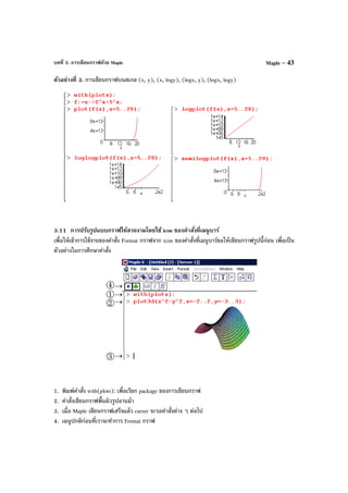
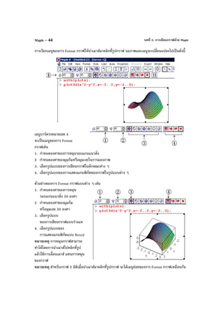
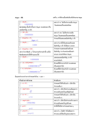
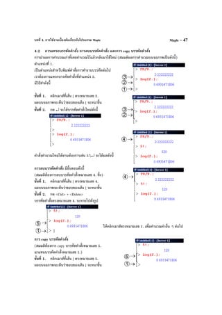
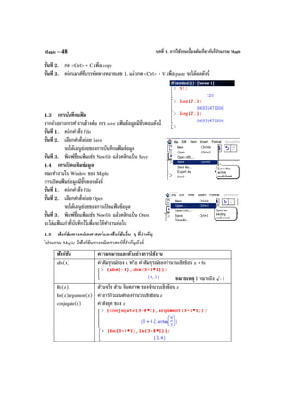

ln(x) ค่าลอกาลิทึมฐาน e
log(x) ค่าลอกาลิทึมฐาน e
log10(x) ค่าลอกาลิทึมฐาน 10
log[b](x) ค่าลอกาลิทึมฐาน b
a mod b
modp(a, b)
mods(a, b)
เศษเหลือจากการหาร a ด้วยจํานวนเต็ม b
เศษเหลือจากการหาร a ด้วยจํานวนเต็ม b (เศษที่มีค่าเป็นบวก)
เศษเหลือจากการหาร a ด้วยจํานวนเต็ม b (เศษที่มีค่าเป็นลบ)
sign(พหุนาม)
signum(x)
เท่ากับ +1 ถ้า สัมประสิทธิ์นํา na > 0 และเท่ากับ –1 ถ้า na < 0
เท่ากับ +1 ถ้า x > 0 และเท่ากับ –1 ถ้า x < 0
และ signum(0)= 0, sign(0) = 0
sqrt(x) รากที่ 2 ของ x](https://image.slidesharecdn.com/bookmathcadmathemeticamatlapmaple-160531122930/85/Book-mathcad-mathematica-matlap-maple-368-320.jpg)
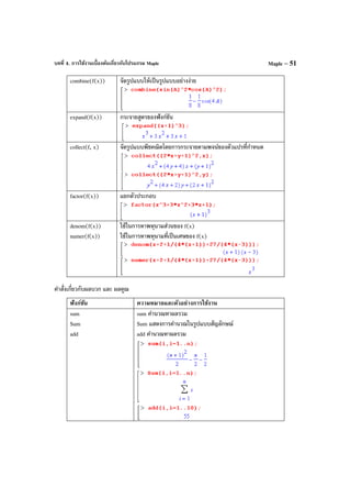

D(f)(a)
(D@@k)(f)
ดิฟเฟอเรนเชียลของ f
D[i](f) = ดิฟเฟอเรนเชียลของ f เทียบกับตัวแปรลําดับที่ i
และ D[](f) คือ f
ดิฟเฟอเรนเชียลของ f ที่ x = a
ดิฟเฟอเรนเชียล )k(
D (f)](https://image.slidesharecdn.com/bookmathcadmathemeticamatlapmaple-160531122930/85/Book-mathcad-mathematica-matlap-maple-372-320.jpg)
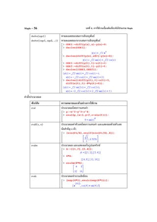
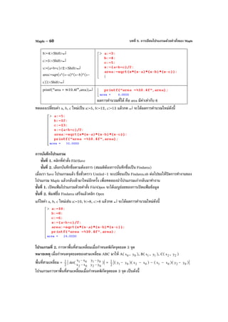
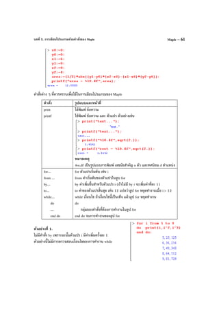
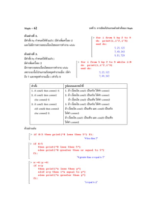
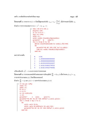
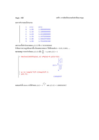
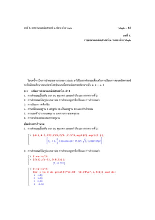
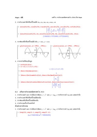
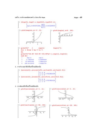
![บทที่ 6. การคํานวณคณิตศาสตร์ ม. ปลาย ด้วย MapleMaple – 70
4. การคํานวณเกี่ยวกับเมทริกซ์
การบวกเมทริกซ์ การคูณเมทริกซ์ สเกลาร์คูณเมทริกซ์ ค่ากําหนดของเมทริกซ์
การหาผลเฉลยของระบบสมการ 2x + 3y = 2
5x + 8y = 1
การแปลงแถวเมทริกซ์ โดยใช้คําสั่ง with(LinearAlgebra) เรียก package การคํานวณเกี่ยวกับการแปลงแถว
RowOperation(A, i, k) คือแถวที่ i ถูกคูณด้วยค่าคงตัว k
RowOperation(A, [i, j], inplace = true) คือการสลับแถว i กับ j
RowOperation(A, [i, j], k) คือแถวที่ i ถูกบวกด้วย k เท่าของแถวที่ j](https://image.slidesharecdn.com/bookmathcadmathemeticamatlapmaple-160531122930/85/Book-mathcad-mathematica-matlap-maple-389-320.jpg)
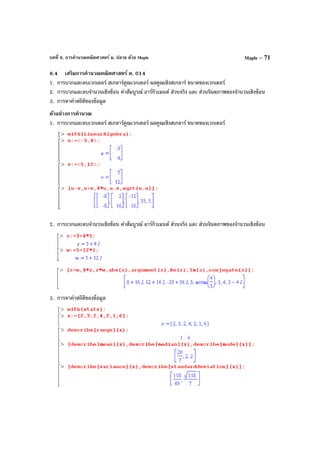
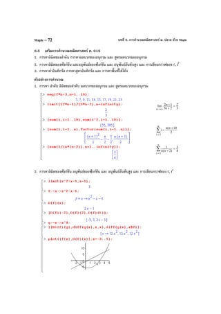
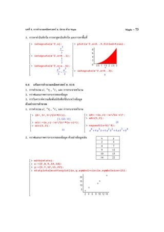
![บทที่ 6. การคํานวณคณิตศาสตร์ ม. ปลาย ด้วย MapleMaple – 74
3. การวิเคราะห์ความสัมพันธ์เชิงฟังก์ชันระหว่างข้อมูล
สมการแสดงความสัมพันธ์ของข้อมูลคือ y = 464
699 x + 464
23 = 1.50647x + 0.049596
6.7 Maple กับการเฉลยข้อสอบคณิตศาสตร์ Entrance
ข้อสอบคณิตศาสตร์ 1. มีนาคม 2546 ข้อ 18.
0x
lim
→ 3
x
1 [ x1+ – x1− – )x1)(x1( 2
−+ + )x1)(x1( 2
−− ] มีค่าเท่ากับข้อใดต่อไปนี้
1. 0 2. 4
1
3. 2
1 4. 1
การคํานวณด้วย Maple
เพราะฉะนั้นตอบข้อ 3.
ข้อสอบคณิตศาสตร์ 2. มีนาคม 2546 ข้อ 11.
ถ้า xsin1
1
−
+ xsin1
1
+
= 8 โดยที่ π < x <
2
3π แล้ว sin x + cos2x + tan3x มีค่าเท่ากับข้อใดต่อไปนี้
1. 2
13 −
2. 2
13 +
3. 2
13 −−
4. 2
13 +−
การคํานวณด้วย Maple
เพราะฉะนั้นตอบข้อ 3.
ข้อสอบคณิตศาสตร์ 1. มีนาคม 2545 ข้อ 2.
2
sin−
1 +
2sin2 –
3sin2 + ... –
89sin2 +
90sin2 มีค่าเท่ากับเท่าใด
การคํานวณด้วย Maple
เพราะฉะนั้น 2
sin−
1 +
2sin2 –
3sin2 + ... –
89sin2 +
90sin2 มีค่าเท่ากับ 0.5](https://image.slidesharecdn.com/bookmathcadmathemeticamatlapmaple-160531122930/85/Book-mathcad-mathematica-matlap-maple-393-320.jpg)
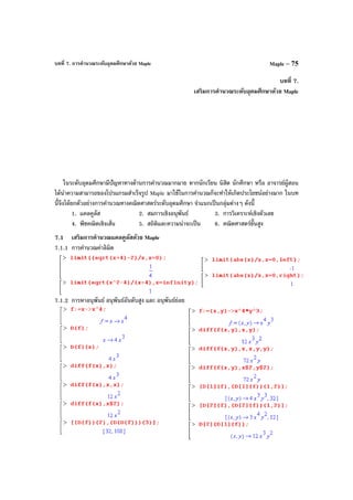
![บทที่ 7. การคํานวณระดับอุดมศึกษาด้วย MapleMaple – 76
7.1.3 การคํานวณปริพันธ์ ผลการคํานวณเป็นสูตร และ ผลการคํานวณเป็นตัวเลข
7.1.4 กราฟของฟังก์ชัน f, f′ และ f′′
7.1.5 การหาผลบวกรีมันน์ (Riemann sum) เช่นผลบวกรีมันน์ของ f(x) = 2
x – 4x + 6 บนช่วง [1, 3]
หมายเหตุ ค่าของ dx)6x4x(
2
3
1
+−∫ = 3
14](https://image.slidesharecdn.com/bookmathcadmathemeticamatlapmaple-160531122930/85/Book-mathcad-mathematica-matlap-maple-395-320.jpg)
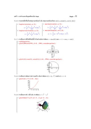
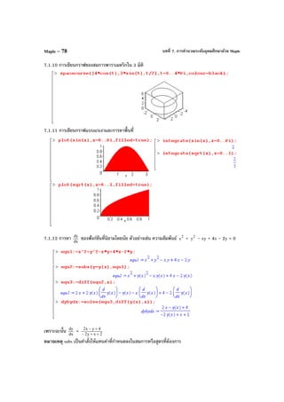
![บทที่ 7. การคํานวณระดับอุดมศึกษาด้วย Maple Maple – 79
7.1.13 การประมาณค่าอินทิกรัลโดยใช้ผลบวกรีมันน์ จําแนกเป็นผลบวกซ้าย (left sum) ผลบวกขวา (right
sum) และ ผลบวกจุดกึ่งกลาง (middle sum) ตัวอย่างเช่น กําหนดให้ f(x) = 2
x + 4 บนช่วง [1, 5]
1. กําหนดฟังก์ชัน
2. เรียก package การเขียนกราฟ
3. เรียก package student
4. คําสั่ง leftbox(f(x), x=a..b, n)
เขียนกราฟแท่งแสดง
พื้นที่ใต้โค้ง y = f(x) บนช่วง [a, b]
โดยแบ่งช่องย่อยออกเป็น n ส่วน
และใช้ความสูงของแท่งสี่เหลี่ยม
จากค่าฟังก์ชันของจุดทางซ้ายของช่วงย่อย
5. leftsum(f(x), x=a..b, n) เป็นคําสั่งหาผลบวก
ของพื้นที่สี่เหลี่ยมทั้งหมดที่เกิดจาก
คําสั่ง leftbox(f(x), x=a..b, n)
6. คําสั่ง middletbox(f(x), x=a..b, n) เขียนกราฟแท่งแสดงพื้นที่ใต้โค้ง y = f(x) บนช่วง [a, b] โดยแบ่ง
ช่องย่อยออกเป็น n ส่วน และใช้ความสูงของแท่งสี่เหลี่ยมจากค่าฟังก์ชันของจุดกึ่งกลางของช่วงย่อย
7. middlesum(f(x), x=a..b, n) เป็นคําสั่งหาผลบวกของพื้นที่สี่เหลี่ยมทั้งหมดที่เกิดจากคําสั่ง
middlebox(f(x), x=a..b, n)
8. คําสั่ง rightbox(f(x), x=a..b, n) เขียนกราฟแท่งแสดงพื้นที่ใต้โค้ง y = f(x) บนช่วง [a, b] โดยแบ่งช่อง
ย่อยออกเป็น n ส่วน และใช้ความสูงของแท่งสี่เหลี่ยม จากค่าฟังก์ชันของจุดทางขวาของช่วงย่อย
9. rightsum(f(x), x=a..b, n) เป็นคําสั่งหาผลบวกของพื้นที่สี่เหลี่ยมทั้งหมดที่เกิดจากคําสั่ง
rightbox(f(x), x=a..b, n)](https://image.slidesharecdn.com/bookmathcadmathemeticamatlapmaple-160531122930/85/Book-mathcad-mathematica-matlap-maple-398-320.jpg)
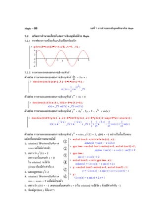
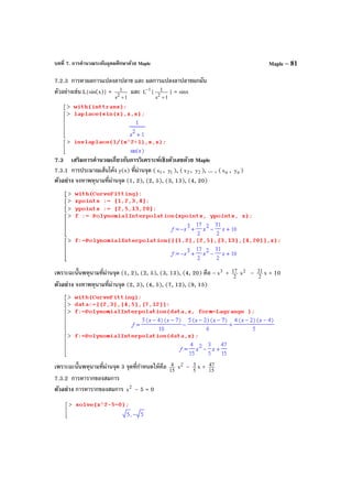
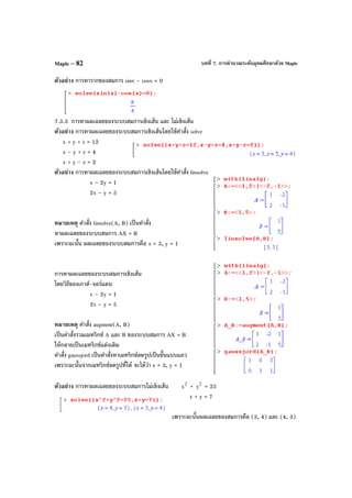
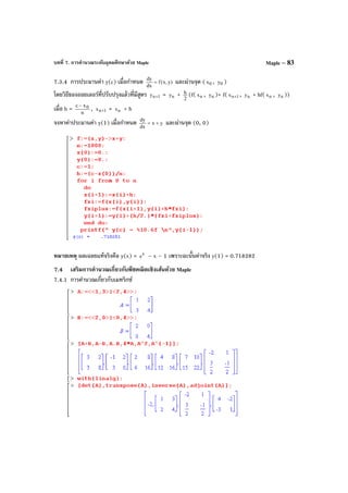
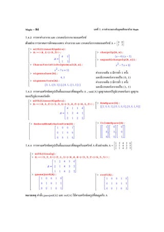
![บทที่ 7. การคํานวณระดับอุดมศึกษาด้วย Maple Maple – 85
7.4.5 การแปลงแถวเมทริกซ์ และการแปลงหลักเมทริกซ์
RowOperation(A, i, k) คือการแปลงแถว ค่าคงตัว k คูณแถวที่ i
RowOperation(A, [i, j], c)
คือการแปลงแถว แถวที่ i ถูกบวกด้วย c เท่าของแถวที่ j
RowOperation(A, [i, j]) คือการแปลงแถว สลับแถว i กับ j
ในทํานองเดียวกัน
ColumnOperation(A, i, k)
คือการแปลงหลัก ค่าคงตัว k คูณหลัก i
ColumnOperation(A, [i, j], c)
คือการแปลงหลัก หลักที่ i ถูกบวกด้วย c เท่าของหลักที่ j
ColumnOperation(A, [i, j])
คือการแปลงหลัก สลับหลักที่ i กับ หลักที่ j
นอกจากนั้นยังมีคําสั่ง swaprow(A, i, j) สลับแถวที่ i กับ แถวที่ j
addrow(A, j, i, c) แถวที่ i ถูกบวกด้วย c เท่าของแถวที่ j
mulrow(A, i, k) ค่าคงตัว k คูณแถวที่ i
swapcol(A, i, j) สลับหลักที่ i กับ หลักที่ j
addcol(A, j, i, c) หลักที่ i ถูกบวกด้วย c เท่าของหลักที่ j
mulcol(A, i, k) ค่าคงตัว k คูณหลักที่ i
7.4.6 การหามูลฐานเชิงตั้งฉากปกติของ 3
R
โดยใช้กระบวนการของ Gram - Schmidt
ตัวอย่าง กําหนดมูลฐาน { 1v =
1
1
1
, 2v =
1
1
0
, 3v =
1
0
0
}
เพราะฉะนั้นมูลฐานเชิงตั้งฉากปกติคือ { 1u =
577.0
577.0
577.0
, 2u =
−
408.0
408.0
816.0
, 3u =
−
707.0
707.0
0
}](https://image.slidesharecdn.com/bookmathcadmathemeticamatlapmaple-160531122930/85/Book-mathcad-mathematica-matlap-maple-404-320.jpg)
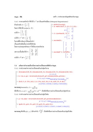
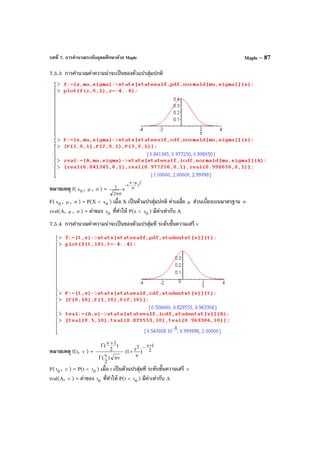
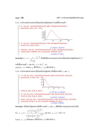
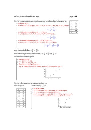
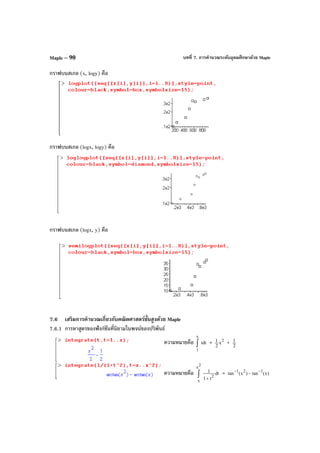
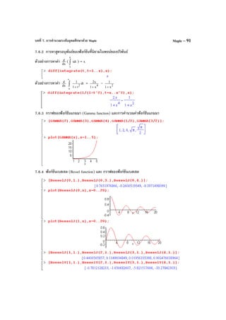
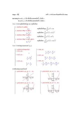
![ฟังก์ชันและคําสั่งที่สําคัญ
Mathematics Mathcad Mathematica MATLAB Maple
π = 3.141592654 <Ctrl+Shift>+P Pi pi Pi, pi
i = 1− i, j , <Esc>ii<Esc> i I
x , n x x , n x Sqrt[x], x , n x sqrt(x) sqrt(x)
e = 2.7182818, x
e
x
e , exp(x) E^x, Exp[x] exp(x) exp(x)
n! n! Factorial[n], n! factorial(n) factorial(n), n!
การกําหนดสูตร f(x) f(x):=... f[x_]:=... สร้าง f.m file f:=x->...
ลอการิทึม ฐาน 10 log(x) Log[10, x] log(x) log10(x)
ลอการิทึม ฐาน e ln(x) Log[x] log10(x) log(x), ln(x)
sin(x) sin(x) Sin[x] sin(x) sin(x)
cos(x) cos(x) Cos[x] cos(x) cos(x)
tan(x) tan(x) Tan[x] tan(x) tan(x)
sec(x) sec(x) Sec[x] sec(x) sec(x)
cosec(x) csc(x) Csc[x] csc(x) csc(x)
cot(x) cot(x) Cot[x] cot(x) cot(x)
arcsin(x) asin(x) ArcSin[x] asin(x) arcsin(x)
arccos(x) acos(x) ArcCos[x] acos(x) arccos(x)
arctan(x) atan(x) ArcTan[x] atan(x) arctan(x)
arcsec(x) asec(x) ArcSec[x] asec(x) arcsec(x)
arccosec(x) acsc(x) ArcCsc[x] acsc(x) arccsc(x)
arccot(x) acot(x) ArcCot[x] acot(x) arccot(x)
ค่าสัมบูรณ์ | x | Abs[x] abs(x) abs(x)
อาร์กิวเมนต์ของ z arg(z) Arg[z] angle(z) argument(z)
ส่วนจริงของ z Re(z) Re[z] real(z) Re(z)
ส่วนจินตภาพของ z Im(z) Im[z] imag(z) Im(z)
สังยุคของ z z Conjugate[z] conj(z) conjugate(z)
det(A) | A | Det[A] det(A) det(A)
เมทริกซ์ 1
A
− A^-1 Inverse[A] inv(A), A^-1 inverse(A)
ค่าเจาะจงของ A eigenvals(A) Eigenvalues[A] [V, D] = eig(A) eigenvalues(A)
เวกเตอร์เจาะจงของ A eigenvecs(A) Eigenvectors[A] [V, D] = eig(A) eigenvectors(A)
ขนาดของเวกเตอร์ u | u | Sqrt[u.u] norm(u) norm(u, 2)
u dot v u*v, yx
⋅ u.v, Dot[u, v] dot(u, v) u.v
DotProduct(u, v)
u cross v ( vu × ) yx
× , <Ctrl>+8 Cross[u, v] cross(u, v) CrossProduct(u,v)](https://image.slidesharecdn.com/bookmathcadmathemeticamatlapmaple-160531122930/85/Book-mathcad-mathematica-matlap-maple-412-320.jpg)
![ฟังก์ชันและคําสั่งที่สําคัญ
Mathematics Mathcad Mathematica MATLAB Maple
ผลบวก Σ Sum sum, symsum Sum, sum, add
ผลคูณ Π Product prod product, Product
ลิมิต Limit limit limit
อนุพันธ์ D, Dt diff Diff, diff, D
อินทิกรัล Integrate int Int, int
อนุกรมเทย์เลอร์ series Series taylor series, taylor
ผลการแปลงลาปลาซ laplace LaplaceTransform laplace laplace
ผลการแปลง
ลาปลาซผกผัน
invlaplace InverseLaplaceTra
nsform
ilaplace invlaplace
ฟังก์ชันแกมมา Γ(x) Gamma[x] gamma(x) GAMMA(x)
ฟังก์ชันเบสเซล J0, J1, Jn
Y0, Y1, Yn
BesselJ, BesselY bessej, bessely BesselJ, BesselY
ฟังก์ชันเลอจองด์ leg(n, x) LegendreP[n, z] legendre LegendreP
กราฟบนระนาบ XY Plot plot, ezplot plot
กราฟพิกัดเชิงขั้ว PolarPlot polar, ezpolar polarplot
กราฟ 3 มิติ Plot3D surf, ezsurf plot3d
กราฟ contour ContourPlot
ContourPlot3D
contour, ezsurfc contourplot
contourplot3d
กราฟ scatter 3 มิติ Plot3D ezplot3 scatterplot
กราฟของ
สมการอิงตัวแปรเสริม
ParametricPlot
ParametricPlot3D
ezplot plot
spacecurve
การจัดรูปพีชคณิต simplify Simplify simplify, collect simplify
การกระจาย expand Expand expand expand
การแยกตัวประกอบ factor Factor factor factor
การแยกเศษส่วนย่อย parfrac Apart residue convert
การหารากของสมการ root, lsolve, Find,
polyroots
Solve, FindRoot,
NRoots
solve, roots, fzero solve, fsolve,
rsolve, RootOf,
allvalues
การหาผลเฉลยของ
ระบบสมการ
Given-Find,
lsolve
Solve, NSolve solve, linsolve solve, linsolve
การหาผลเฉลยของ
สมการเชิงอนุพันธ์
odesolve DSolve dsolve dsolve](https://image.slidesharecdn.com/bookmathcadmathemeticamatlapmaple-160531122930/85/Book-mathcad-mathematica-matlap-maple-413-320.jpg)