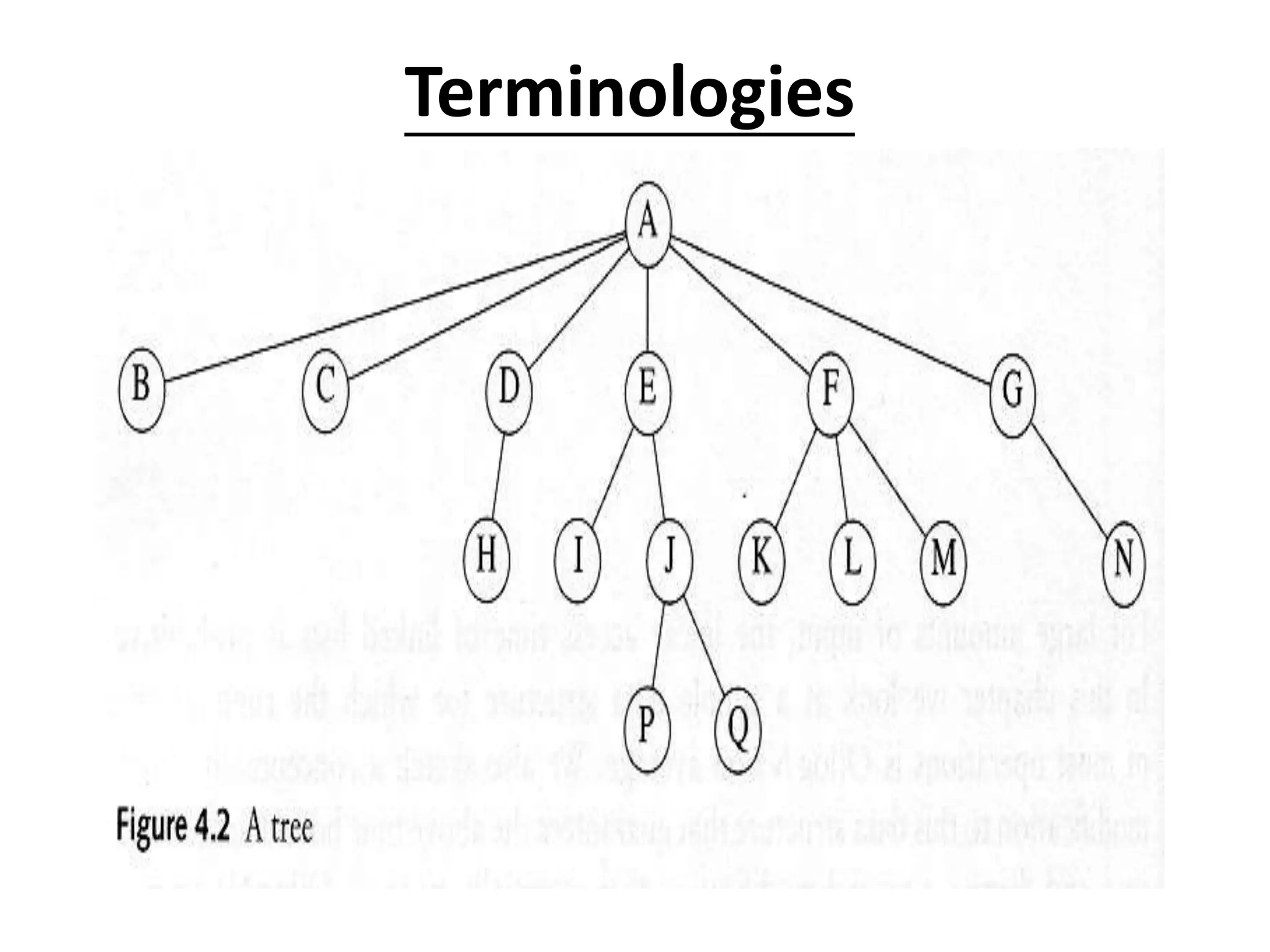
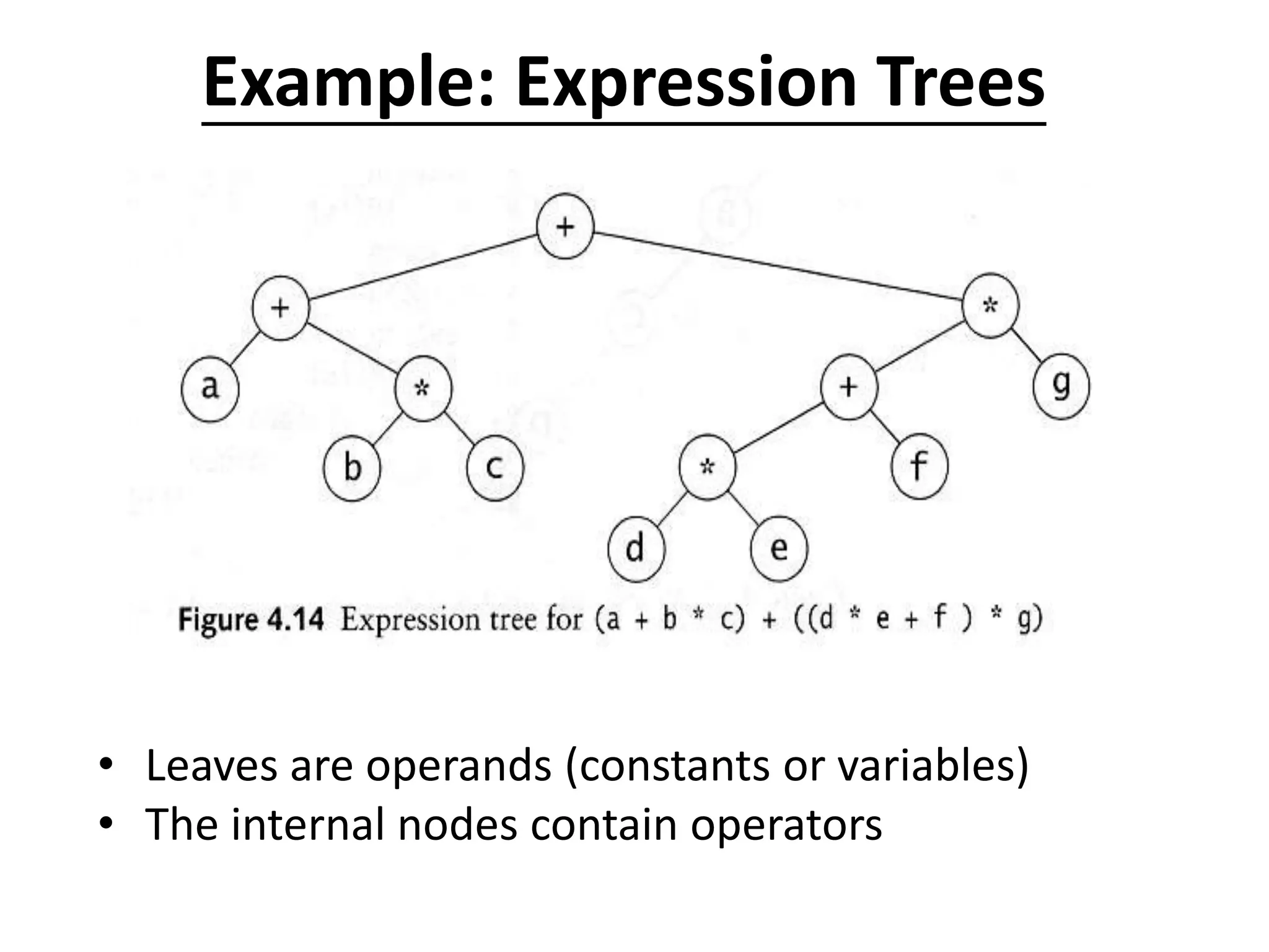
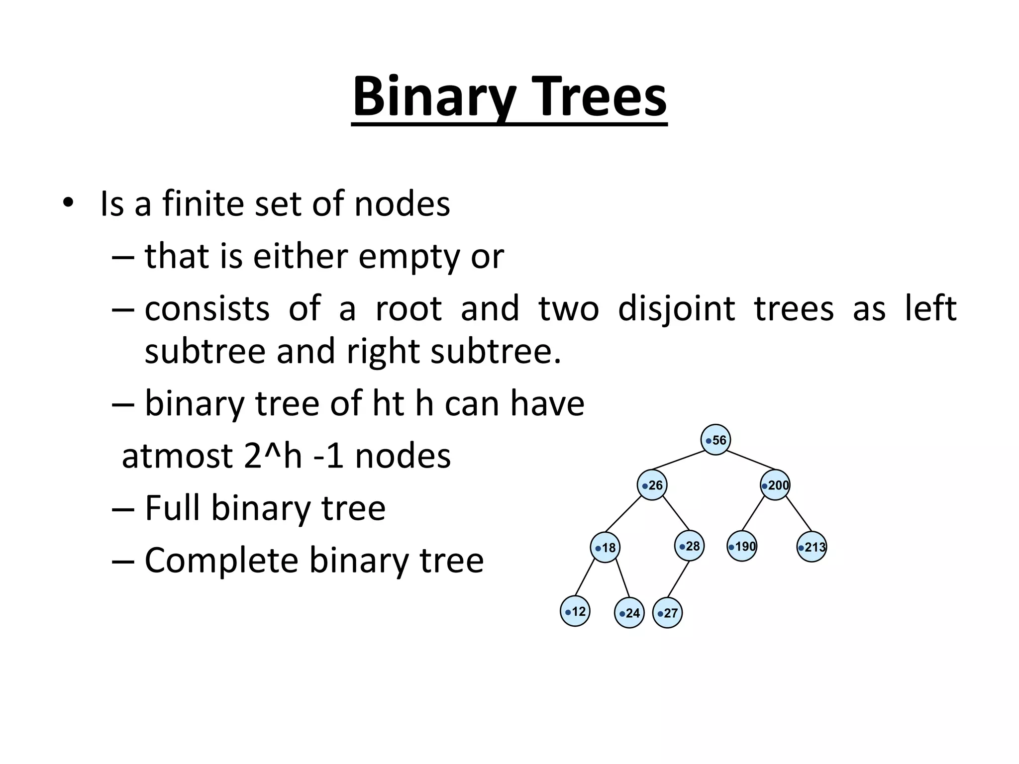
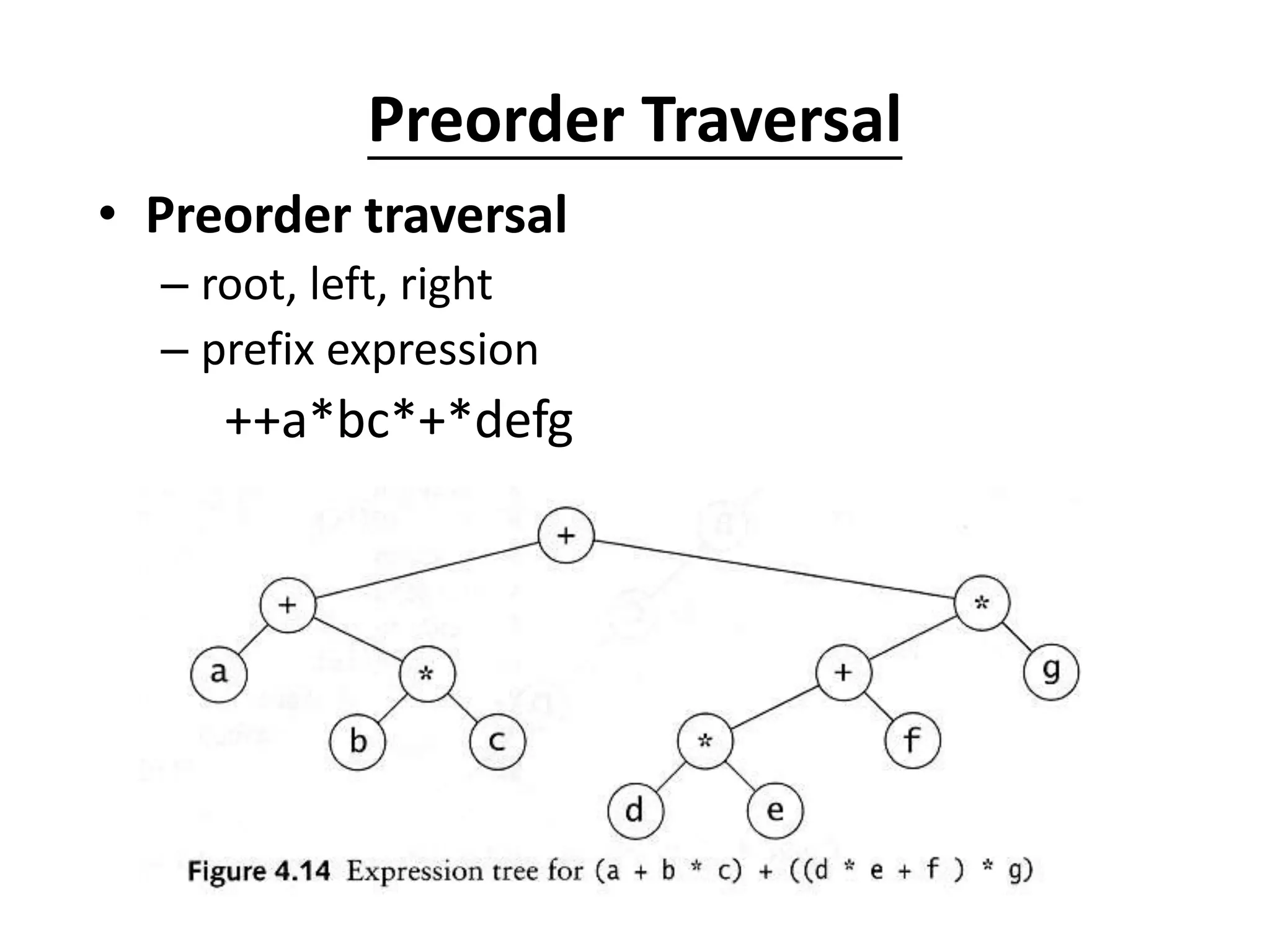
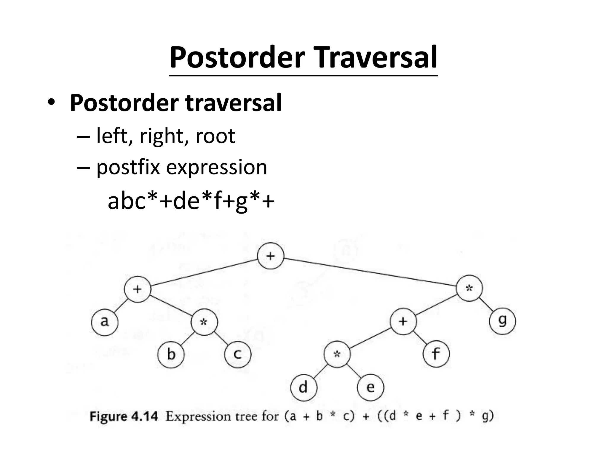
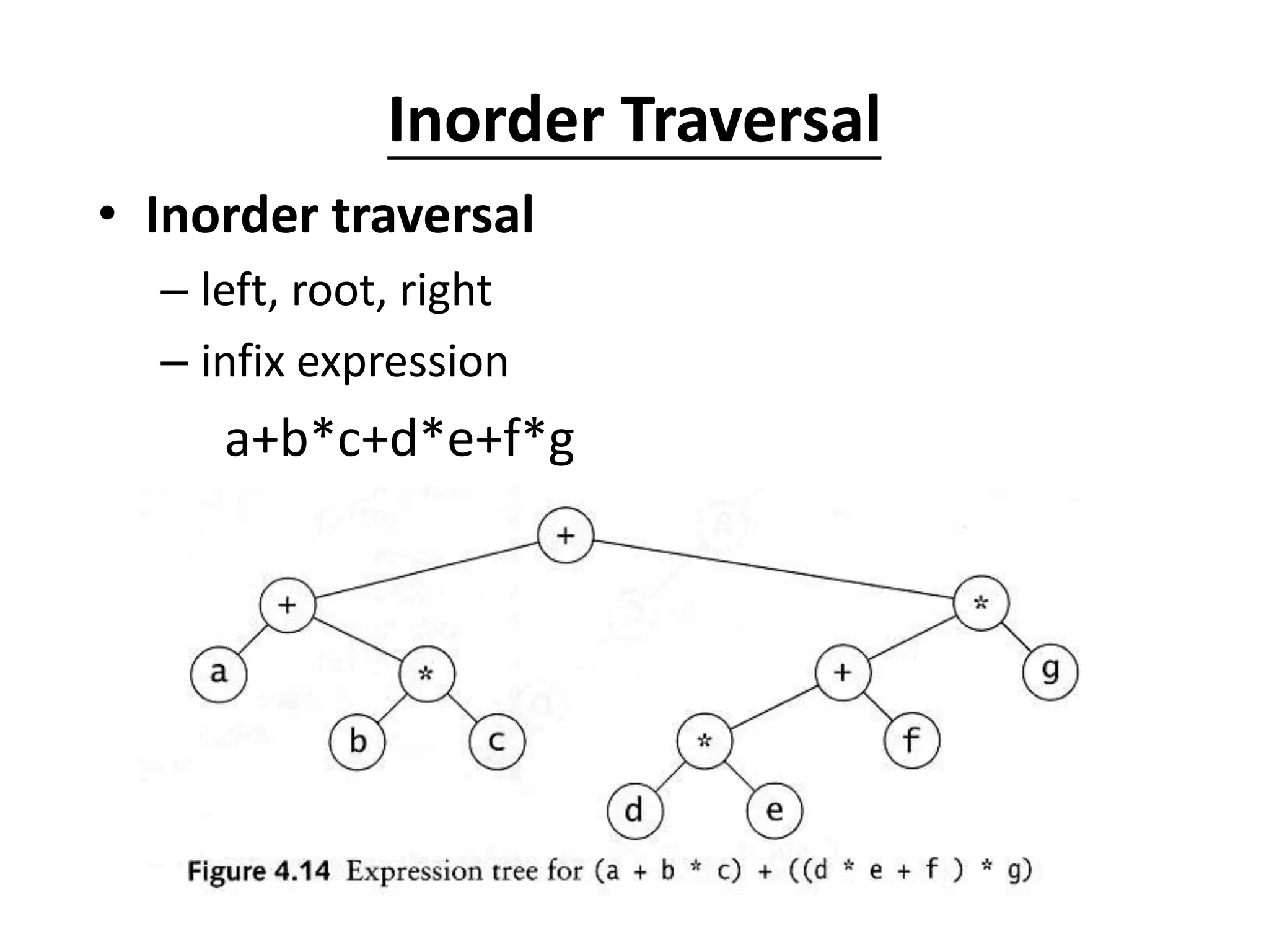
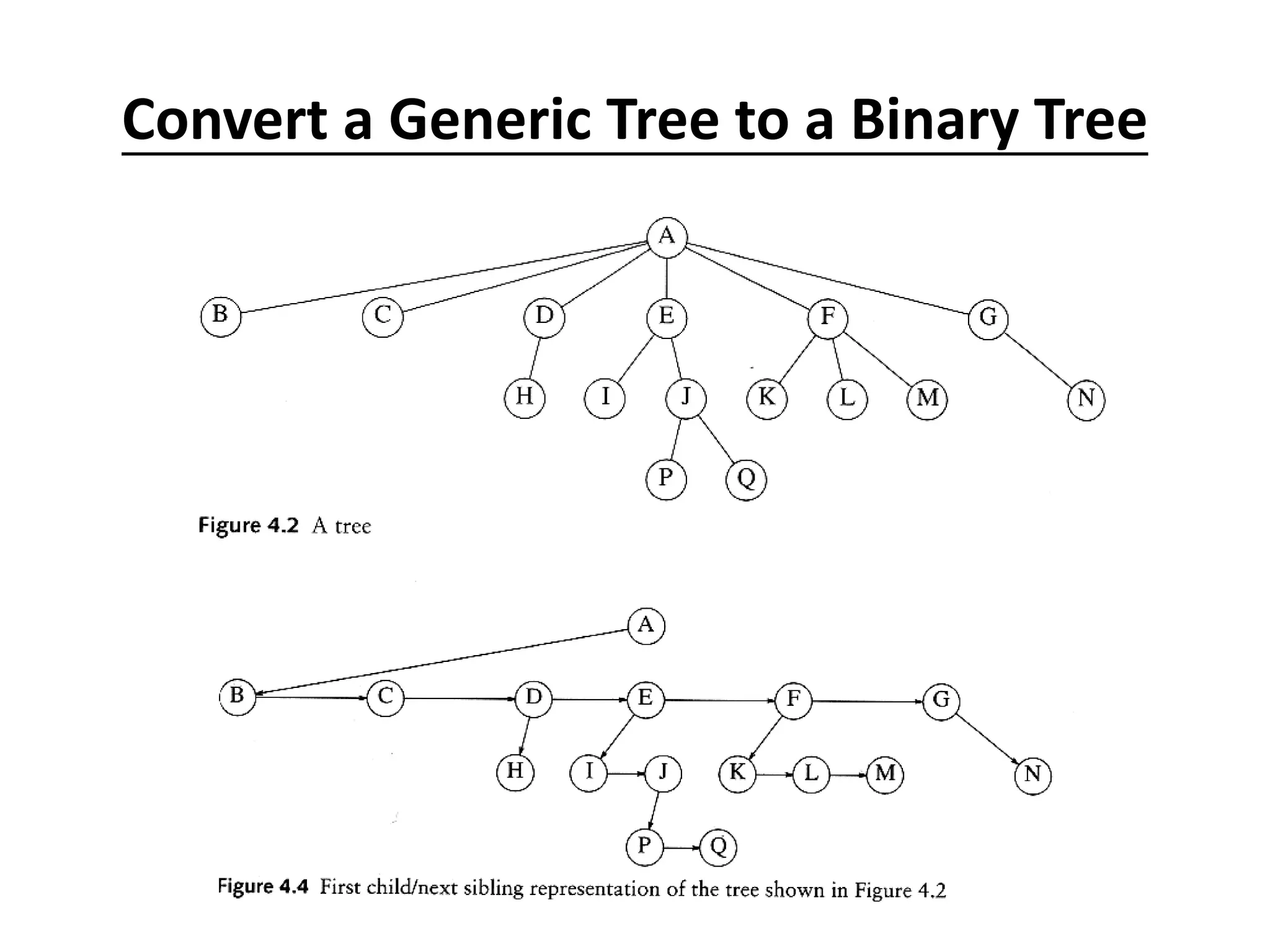
The document defines common tree terminology and describes trees and binary trees. It discusses tree traversal methods including preorder, inorder, and postorder traversal. It also covers binary search trees, including their representation, properties, and common operations like searching, insertion, deletion, finding the minimum/maximum, and finding predecessors and successors. Key operations on binary search trees like searching, insertion, and deletion run in O(h) time where h is the tree height.

1. TREES

2. Trees
• A tree is a collection of nodes
– The collection can be empty
– If not empty, a tree consists of a distinguished
node r (the root), and zero or more nonempty
subtrees T1, T2, ...., Tk, each of whose roots are
connected by a directed edge from r.

3. Terminologies
• Parent
– Immediate predecessor of a node
• Child
– Immediate successors of a node (left child,right
child)
• Leaves
– Leaves are nodes with no children
• Sibling
– nodes with same parent

4. Terminologies
• Level
– Rank in the hierarchy
• Length of a path
– number of edges on the path
• Height of a node(Depth )
– max no of nodes in a path starting from the
root node to a leaf node.
• Degree
– Max no of children that is possible for a node
• Ancestor and descendant
– If there is a path from n1 to n2
– n1 is an ancestor of n2, n2 is a descendant of
n1
– Proper ancestor and proper descendant

5. Terminologies

6. Example: Expression Trees
• Leaves are operands (constants or variables)
• The internal nodes contain operators

7. Binary Trees
• Is a finite set of nodes
– that is either empty or
– consists of a root and two disjoint trees as left
subtree and right subtree.
– binary tree of ht h can have
atmost 2^h -1 nodes
– Full binary tree
– Complete binary tree
56
26 200
18 28 190 213
12 24 27

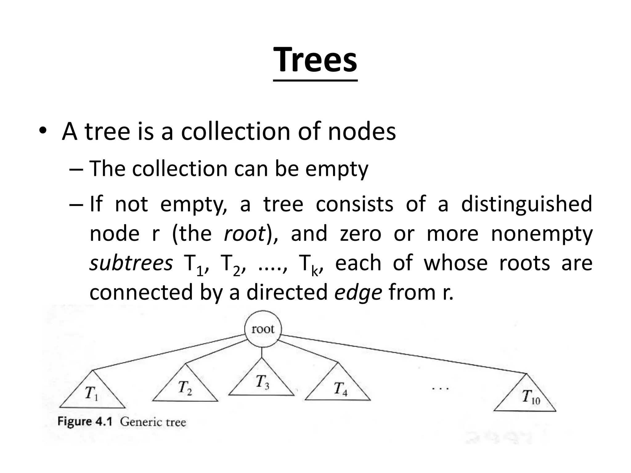
8. Binary Tree Representation
• Linear Representation
– Parent (i)=[i/2]
– Lchild (i)= 2 * i
– Rchild(i)=(2*i) +1
• Linked Representation
– three fields
• leftchild
• data
• rightchild

9. Tree Traversal
• Used to print out the data in a tree in a certain
order
• Pre-order traversal
• Post-order traversal
• In-order traversal

10. Preorder Traversal
• Preorder traversal
– root, left, right
– prefix expression
++a*bc*+*defg

11. Postorder Traversal
• Postorder traversal
– left, right, root
– postfix expression
abc*+de*f+g*+

12. Inorder Traversal
• Inorder traversal
– left, root, right
– infix expression
a+b*c+d*e+f*g

13. Convert a Generic Tree to a Binary Tree

14. Binary Search Trees
• Binary search tree
– Every node has a unique key.
– The keys in a nonempty left subtree are smaller
than the key in the root .
– The keys in a nonempty right subtree are
greater than the key in the root .
– The left and right subtrees are also binary
search trees.

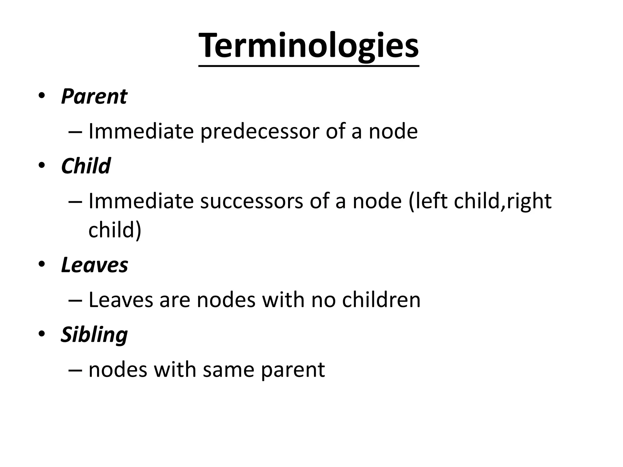
15. BST – Representation
• Represented by a linked data structure of nodes.
• root(T) points to the root of tree T.
• Each node contains fields:
– key
– left – pointer to left child: root of left subtree.
– right – pointer to right child : root of right subtree.
– p – pointer to parent. p[root[T]] = NIL (optional).

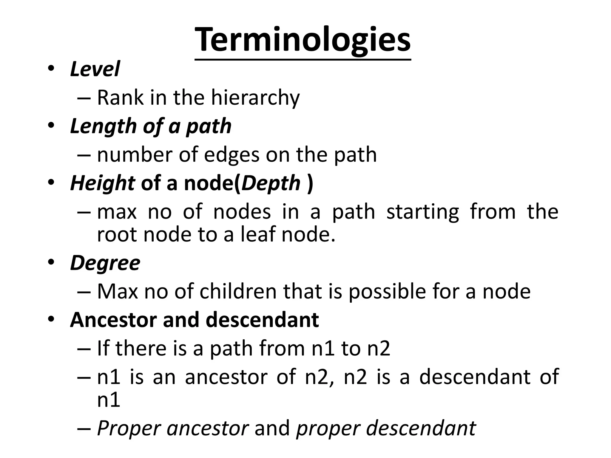
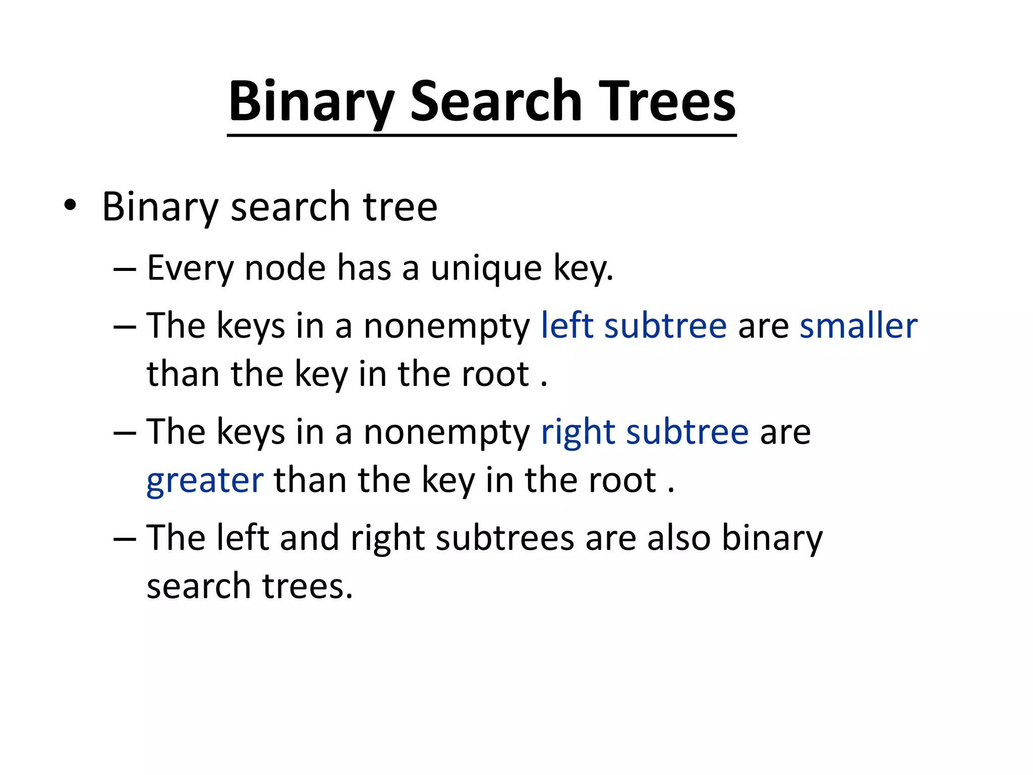
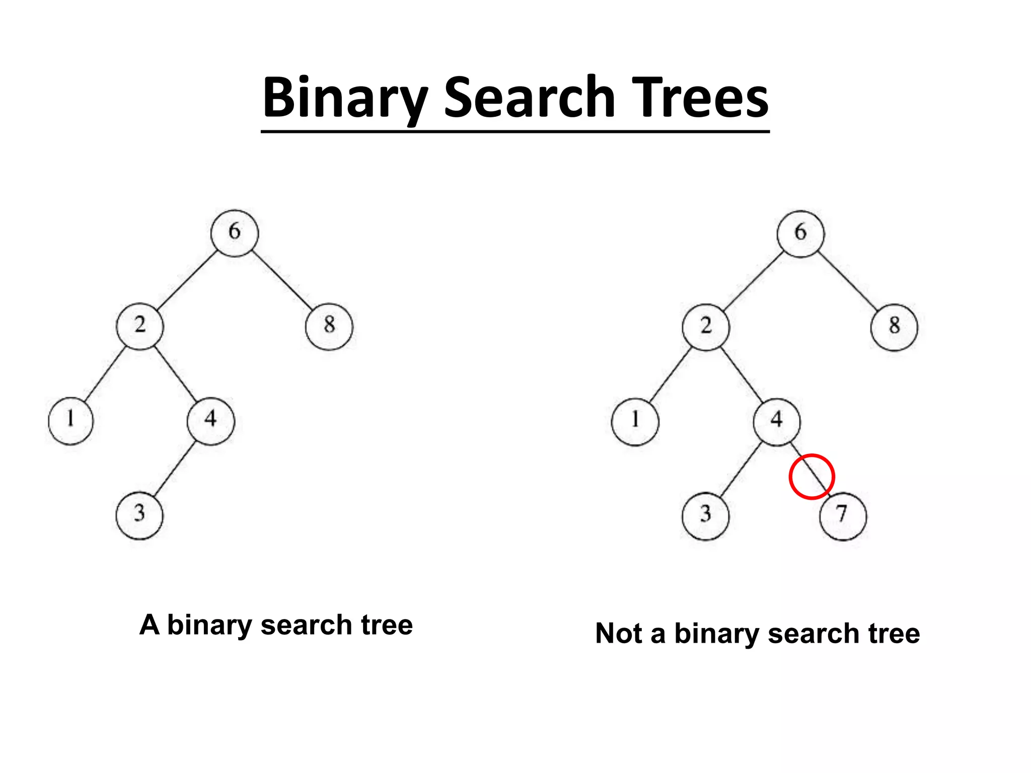
16. Binary Search Tree Property
• Stored keys must satisfy
the binary search tree
property.
–  y in left subtree of
x, then key[y] 
key[x].
–  y in right subtree
of x, then key[y] 
key[x].
56
26 200
18 28 190 213
12 24 27

17. Binary Search Trees
A binary search tree Not a binary search tree

18. Binary Search Trees
• Average depth of a node is O(log N)
• Maximum depth of a node is O(N)
The same set of keys may have different BSTs

19. Querying a Binary Search Tree
• Pseudocode
– if the tree is empty
return NULL
– else if the item in the node equals the target
return the node value
– else if the item in the node is greater than the
target
return the result of searching the left subtree
– else if the item in the node is smaller than the
target
return the result of searching the right subtree

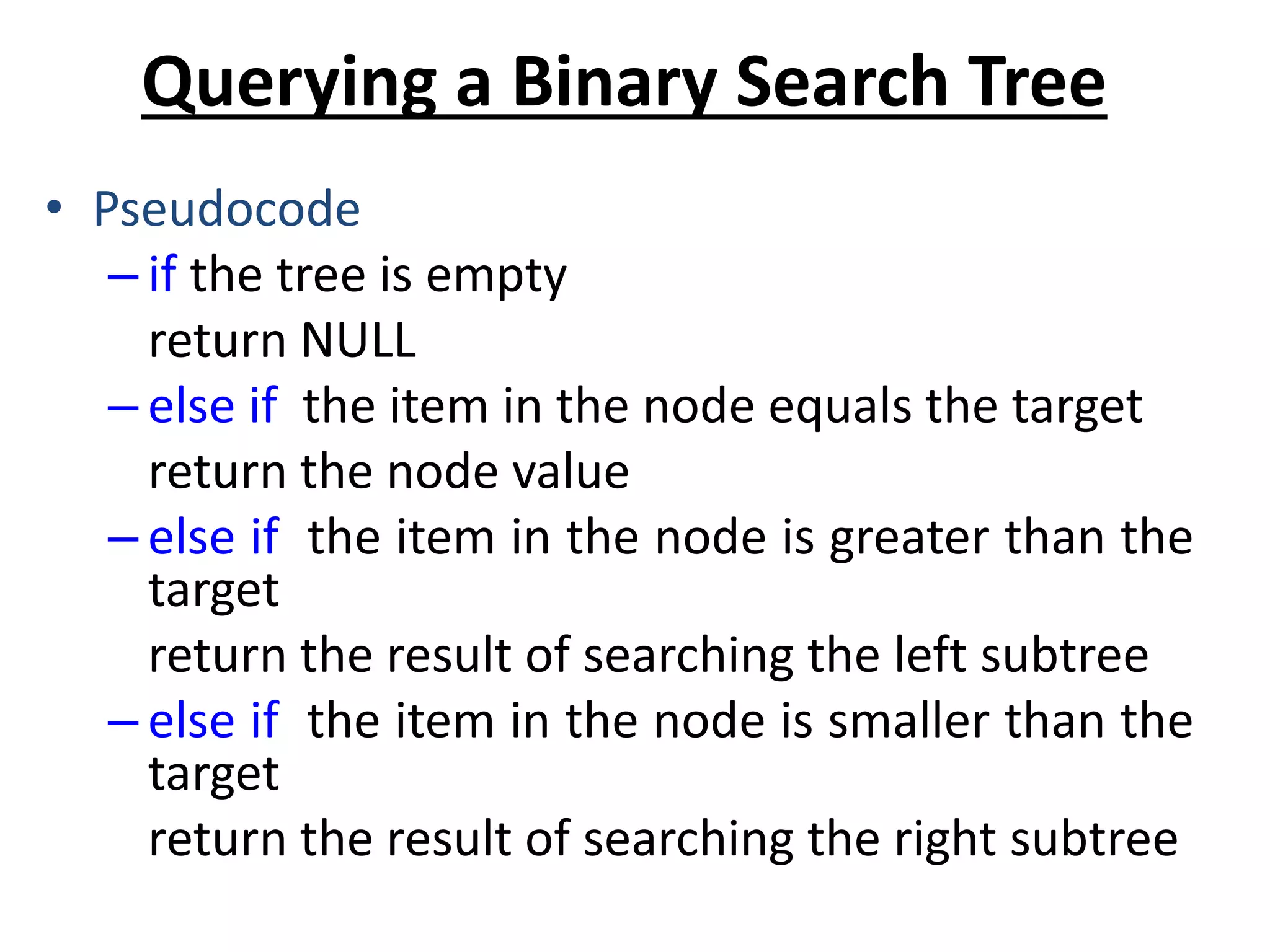
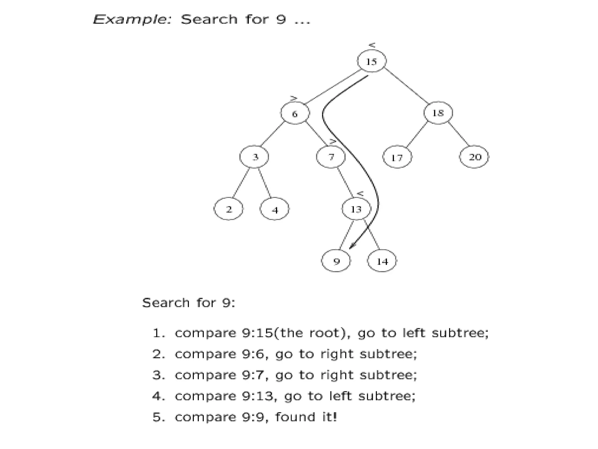
20. Tree Search
Tree-Search(x, k)
1. if x = NIL or k = key[x]
2. then return x
3. if k < key[x]
4. then return Tree-Search(left[x], k)
5. else return Tree-Search(right[x], k)
Running time: O(h)
56
26 200
18 28 190 213
12 24 27

21. Iterative Tree Search
Iterative-Tree-Search(x, k)
1. while x  NIL and k  key[x]
2. do if k < key[x]
3. then x  left[x]
4. else x  right[x]
5. return x
The iterative tree search is more efficient on most computers.
The recursive tree search is more straightforward.
56
26 200
18 28 190 213
12 24 27

23. Querying a Binary Search Tree
• All dynamic-set search operations can be supported in
O(h) time.
• h = (lg n) for a balanced binary tree (and for an
average tree built by adding nodes in random order.)
• h = (n) for an unbalanced tree that resembles a
linear chain of n nodes in the worst case.

24. Finding Min & Max
Tree-Minimum(x) Tree-Maximum(x)
1. while left[x]  NIL 1. while right[x]  NIL
2. do x  left[x] 2. do x  right[x]
3. return x 3. return x
The binary-search-tree property guarantees that:
» The minimum is located at the left-most node.
» The maximum is located at the right-most node.

25. Predecessor and Successor
• Successor of node x is the node y such that key[y] is the
smallest key greater than key[x].
• The successor of the largest key is NIL.
• Two cases:
– If node x has a non-empty right subtree, then x’s successor is
the minimum in the right subtree of x.
– If node x has an empty right subtree, then:
• As long as we move to the left up the tree (move up
through right children), we are visiting smaller keys.
• x’s successor y is the node that x is the predecessor of (x is
the maximum in y’s left subtree).
• In other words, x’s successor y, is the lowest ancestor of x
whose left child is also an ancestor of x.

26. Pseudo-code for Successor
Tree-Successor(x)
1. if right[x]  NIL
2. then return Tree-Minimum(right[x])
3. y  p[x]
4. while y  NIL and x = right[y]
5. do x  y
6. y  p[y]
7. return y
Code for predecessor is symmetric.
Running time: O(h)
56
26 200
18 28 190 213
12 24 27

27. 27
Predecessor
Def: predecessor (x ) = y, such that key [y] is the
biggest key < key [x]
E.g.: predecessor (15) =
predecessor (9) =
predecessor (7) =
Case 1: left (x) is non empty
predecessor (x ) = the maximum in left (x)
Case 2: left (x) is empty
go up the tree until the current node is a right child:
predecessor (x ) is the parent of the current node
if you cannot go further (and you reached the root):
x is the smallest element
3
2 4
6
7
13
15
18
17 20
9
13
7
6 x
y

28. if tree is empty
create a root node with the new key
else
compare key with the top node
if key = node key
replace the node with the new value
else if key > node key
compare key with the right subtree:
if subtree is empty create a leaf node
else add key in right subtree
else key < node key
compare key with the left subtree:
if the subtree is empty create a leaf node
else add key to the left subtree
BST Insertion

29. 9
7
5
4 6 8
 Case 1: The Tree is Empty
 Set the root to a new node containing the item
 Case 2: The Tree is Not Empty
 Call a recursive helper method to insert the item
10 10 > 7
10 > 9
10
BST Insertion

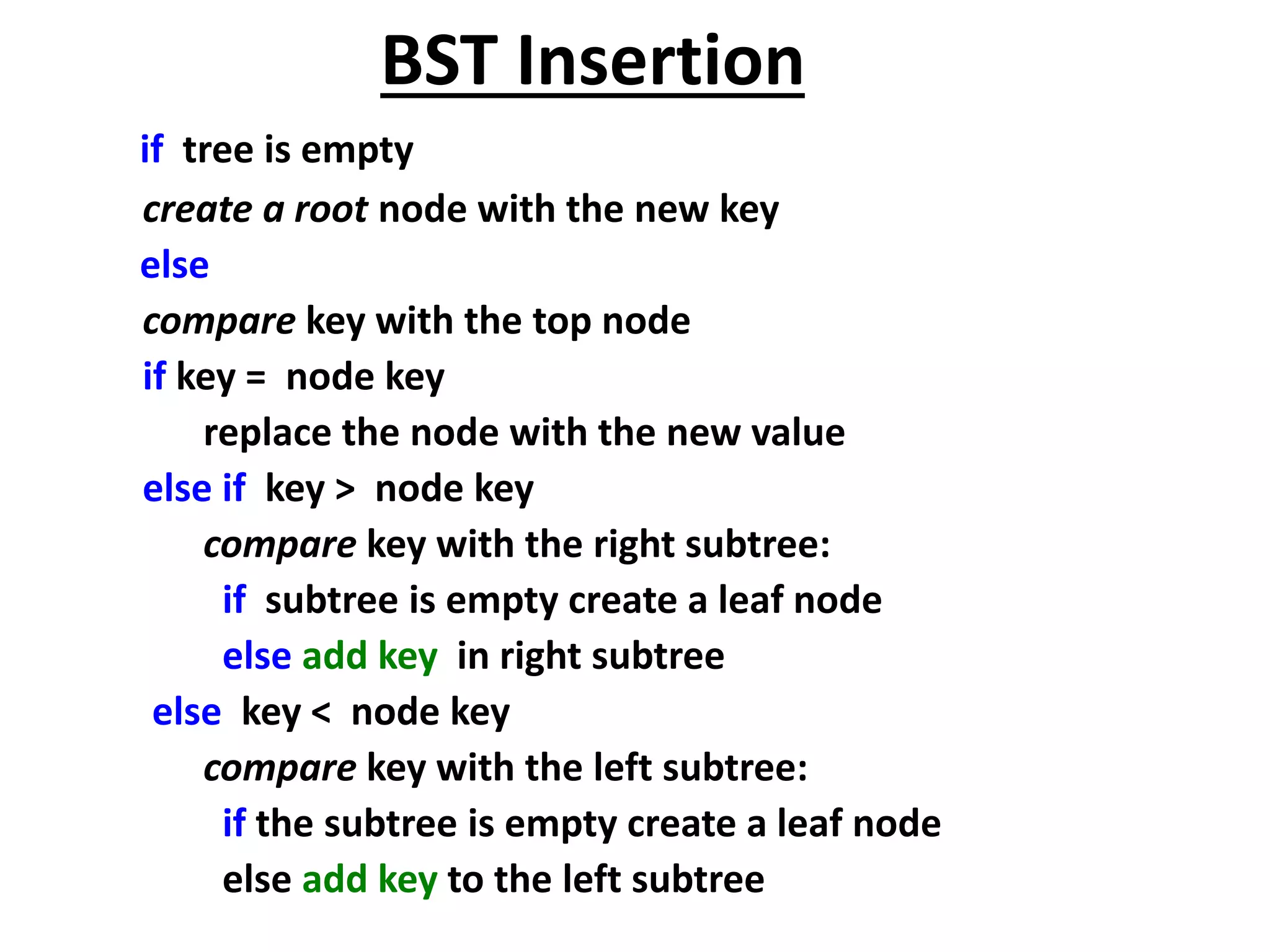
30. BST Insertion – Pseudocode
Tree-Insert(T, z)
y  NIL
x  root[T]
while x  NIL
do y  x
if key[z] < key[x]
then x  left[x]
else x  right[x]
p[z]  y
if y = NIL
then root[t]  z
else if key[z] < key[y]
then left[y]  z
else right[y]  z
• Ensure the binary-
search-tree property
holds after change.
• Insertion is easier than
deletion.
56
26 200
18 28 190 213
12 24 27

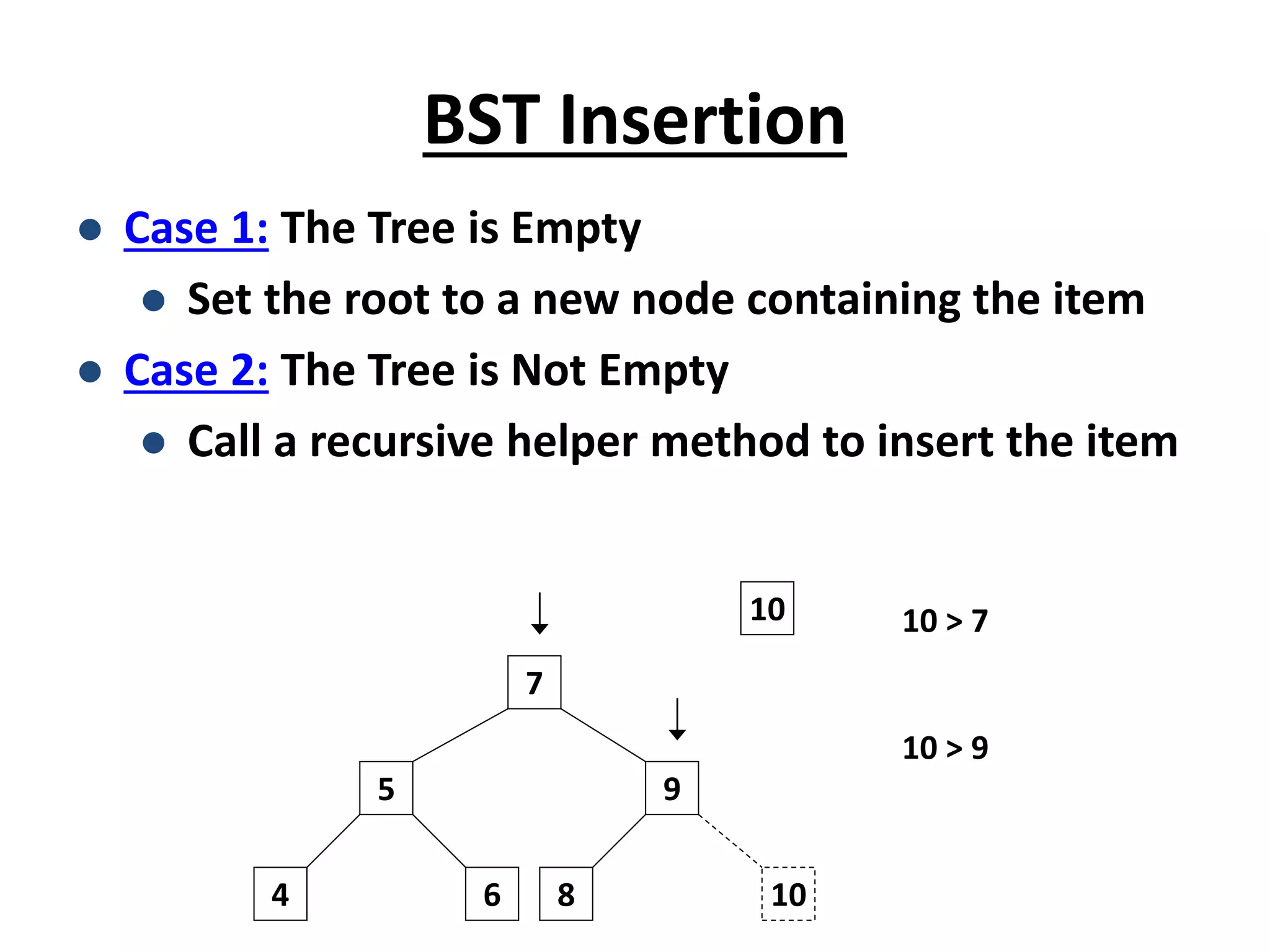
31. Analysis of Insertion
• Initialization: O(1)
• While loop in lines 3-7
searches for place to
insert z, maintaining
parent y.
This takes O(h) time.
• Lines 8-13 insert the
value: O(1)
 TOTAL: O(h) time to
insert a node.
Tree-Insert(T, z)
1. y  NIL
2. x  root[T]
3. while x  NIL
4. do y  x
5. if key[z] < key[x]
6. then x  left[x]
7. else x  right[x]
8. p[z]  y
9. if y = NIL
10. then root[t]  z
11. else if key[z] < key[y]
12. then left[y]  z
13. else right[y]  z

32. I ->if the tree is empty return false
II ->Attempt to locate the node containing the target
using the binary search algorithm
if the target is not found return false
else the target is found, so remove its node:
Case 1: if the node has 2 empty subtrees
-replace the link in the parent with null
Case 2: if the node has a left and a right subtree
- replace the node's value with the max value in
the left subtree
- delete the max node in the left subtree
BST Deletion

33. Case 3: if the node has no left child
-link the parent of the node to the right
(non- empty) subtree
Case 4: if the node has no right child
- link the parent of the target to the left
(non-empty) subtree
BST Deletion

34. 9
7
5
6
4 8 10
9
7
5
6 8 10
Case 1: removing a node with 2 EMPTY SUBTREES
parent
cursor
BST Deletion
Removing 4
replace the link in the
parent with null

35. Case 2: removing a node with 2 SUBTREES
9
7
5
6 8 10
9
6
5
8 10
cursor
cursor
- replace the node's value with the max value in the
left subtree
- delete the max node in the left subtree
4
4
Removing
7
BST Deletion

36. 9
7
5
6 8 10
9
7
5
6 8 10
cursor
cursor
parent
parent
-the node has no left child:
-link the parent of the node
to the right (non-empty) subtree
Case 3: removing a node with 1 EMPTY SUBTREE
BST Deletion

37. 9
7
5
8 10
9
7
5
8 10
cursor
cursor
parent
parent
-the node has no right child:
-link the parent of the node to the
left (non-empty) subtree
Case 4: removing a node with 1 EMPTY SUBTREE
Removing 5
4 4
BST Deletion

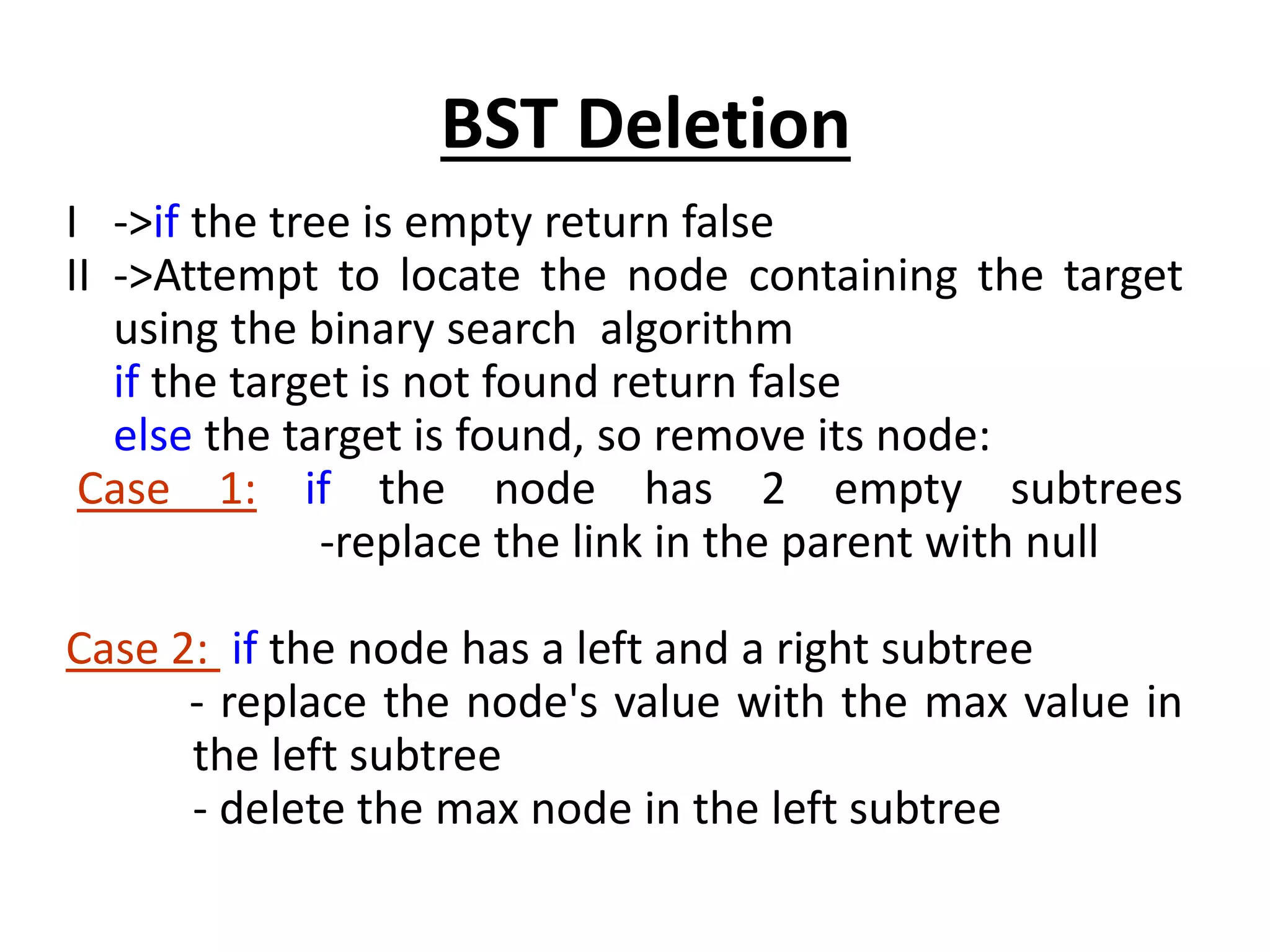
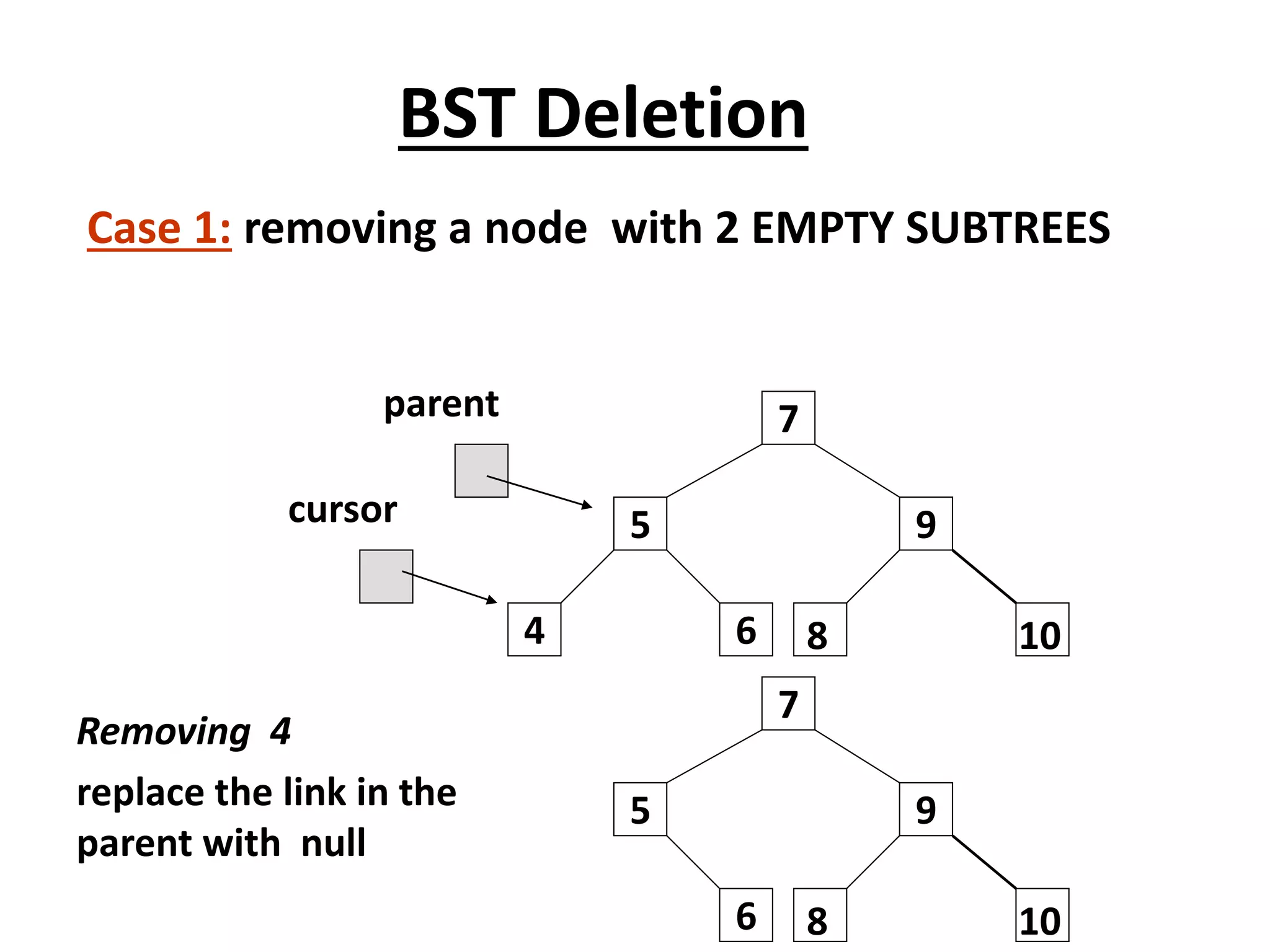
38. Deletion – Pseudocode
TREE-DELETE(T, z)
1. if left[z] = NIL or right[z] = NIL
2. then y ← z
3. else y ← TREE-SUCCESSOR(z)
4. if left[y]  NIL
5. then x ← left[y]
6. else x ← right[y]
7. if x  NIL
8. then p[x] ← p[y]
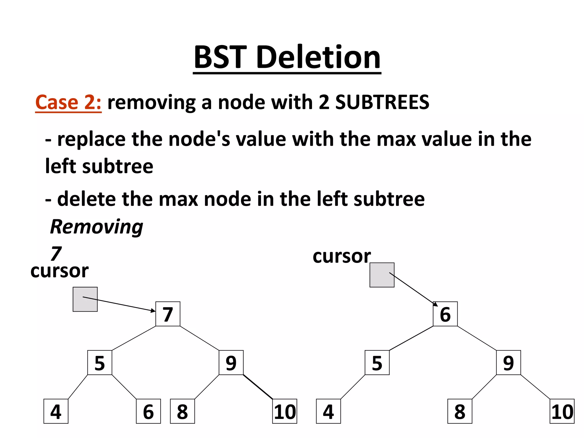
z has one child
z has 2 children
15
16
20
18 23
6
5
12
3
7
10 13
y
x

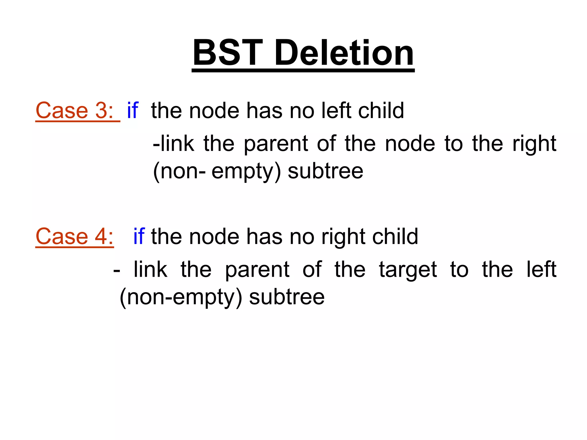
39. Deletion – Pseudocode
TREE-DELETE(T, z)
9. if p[y] = NIL
10. then root[T] ← x
11. else if y = left[p[y]]
12. then left[p[y]] ← x
13. else right[p[y]] ← x
14. if y  z
15. then key[z] ← key[y]
16. copy y’s satellite data into z
17. return y
15
16
20
18 23
6
5
12
3
7
10 13
y
x
Running time: O(h)