Download as PDF, PPTX
![2. Software and documentation.
WEB:
OFICIAL WEB: http://www.r-project.org/index.html
QUICK-R:
http://www.statmethods.net/index.html
BOOKS:
Introductory Statistics with R (Statistics and Computing), P. Dalgaard
[available as manual at R project web]
The R Book, MJ. Crawley
R itself: help() and example()](https://image.slidesharecdn.com/10098418-111109221018-phpapp01/85/Introduction2R-6-320.jpg)
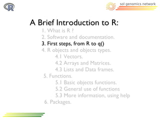
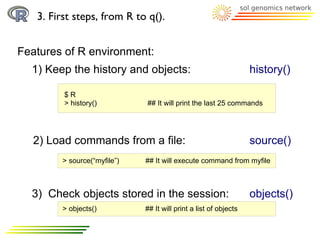
![3. First steps, from R to q().
Two ways to run R:
1) Interactively: q()
$R
> “any R command, as functions, objects ...”
> q() “to exit”
2) Command line
$ R [options] [< infile] [> outfile]
or: R CMD command [arguments]
$ R –vanilla < myRcommands.txt > myRresults.txt](https://image.slidesharecdn.com/10098418-111109221018-phpapp01/85/Introduction2R-8-320.jpg)
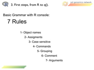
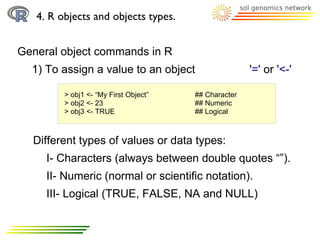
![3. First steps, from R to q().
Basic Grammar with R console:
1) Objects are defined with names.
This names can be composed by alphanumeric
characters, [a-z,0-9], dots '.' and underlines '-'.
Names should start with [a-z] or '.' plus [a-z]
>x
> x_23.test
2) '=' or '<-' signs are used to assign a value to an object
> x <- 100
> y <- 25](https://image.slidesharecdn.com/10098418-111109221018-phpapp01/85/Introduction2R-10-320.jpg)
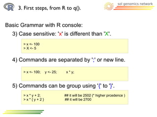
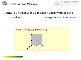
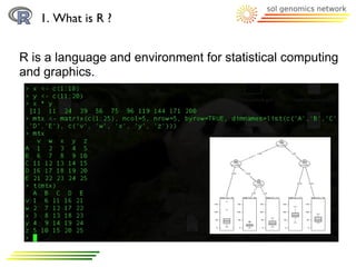
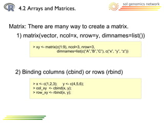
![4.2 Arrays and Matrices.
Array: Arrays are indexed
> xyz <- array(c(1:27), dim=c(3, 3, 3))
> xyz
,,1 First dimension
[,1] [,2] [,3] Second dimension
[1,] 1 4 7
[2,] 2 5 8
[3,] 3 6 9
,,2
[,1] [,2] [,3]
[1,] 10 13 16
[2,] 11 14 17
[3,] 12 15 18
,,3
[,1] [,2] [,3]
[1,] 19 22 25
[2,] 20 23 26
[3,] 21 24 27
Third dimension](https://image.slidesharecdn.com/10098418-111109221018-phpapp01/85/Introduction2R-24-320.jpg)
![4.2 Arrays and Matrices.
Array: Arrays are indexed, so each element is accessible
throught these indexes
> xyz <- array(c(1:27), dim=c(3, 3, 3))
> xyz
> xyz[2,2,2] ## a single numeric element
> xyz[2,2, ] ## a vector (1 dimension array)
> xyz[2, , ] ## a 2 dimension array](https://image.slidesharecdn.com/10098418-111109221018-phpapp01/85/Introduction2R-25-320.jpg)
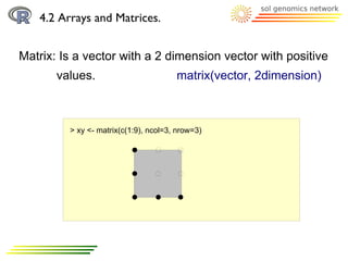
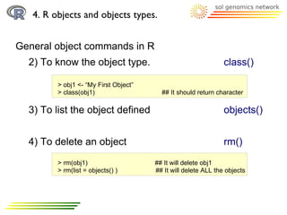
![4.2 Arrays and Matrices.
Matrix: It has indexes too
> xy <- matrix(c(1:9), ncol=3, nrow=3)
> xy
> xy[2,2] ## a single numeric element
> xy[2, ] ## a vector (1 dimension array)
Matrix: Indexes can be replaced by names
> xy <- matrix(c(1:9), ncol=3, nrow=3,
dimnames=list(c(“A”,”B”,”C”), c(“x”, “y”, “z”)))
xyz
A147
B258
C369](https://image.slidesharecdn.com/10098418-111109221018-phpapp01/85/Introduction2R-27-320.jpg)
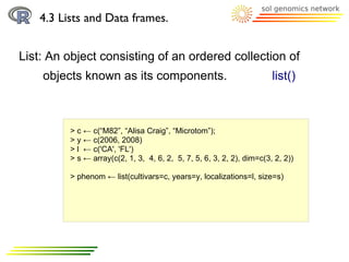
![4.3 Lists and Data frames.
List: Objects in the list are indexed and also can be
accessible using their names
> phenom ← list(cultivars=c, years=y, localizations=l, size=s)
>phenom[ [ 1 ] ]
>phenom$cultivars](https://image.slidesharecdn.com/10098418-111109221018-phpapp01/85/Introduction2R-34-320.jpg)
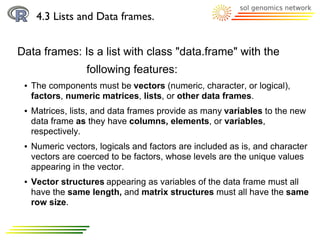
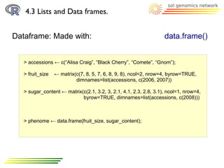
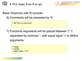
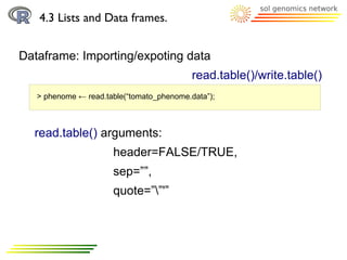
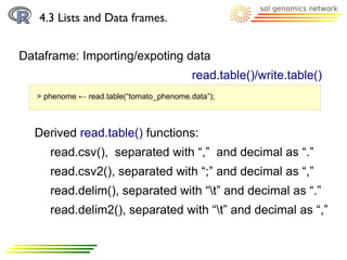
![4.3 Lists and Data frames.
Dataframe: Accessing to the data attach()/detach()
summary()
> phenome ← data.frame(fruit_size, sugar_content);
## As a matrix:
> phenome[1,] ## for a row
> phenome[,1] ## for a column
> phenome[1,1] ## for a single data
## Based in the column names
> phenome$X2007
## To divide/join the data.frame in its columns use attach/detach function
>attach(phenome)
> X2007
>summary(phenome) ## To know some stats about this dataframe](https://image.slidesharecdn.com/10098418-111109221018-phpapp01/85/Introduction2R-37-320.jpg)
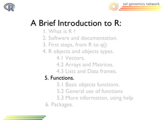
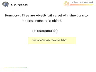
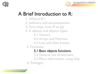
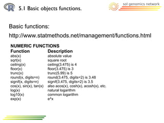
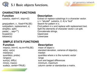

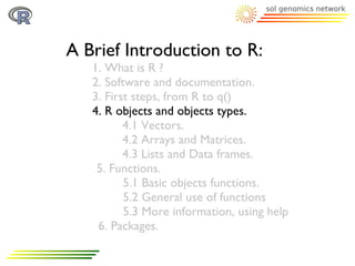
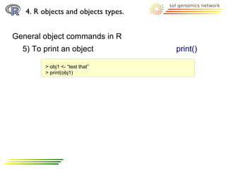
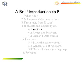
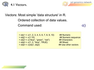
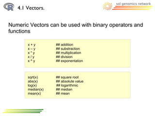
The document provides an introduction to the statistical programming language R. It describes what R is, how to get started using it interactively or via commands, and some basic grammar rules. It also covers different data types in R including vectors, arrays, matrices, and lists, as well as functions for creating, manipulating, and accessing different object types. The introduction aims to provide new users with foundational knowledge for using R.