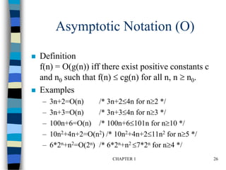
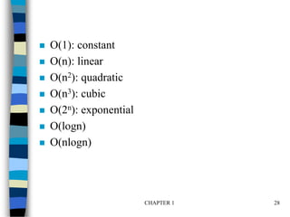
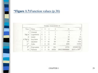
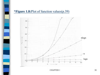
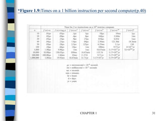
This document discusses algorithms and data structures. It begins by defining an algorithm as a set of instructions to accomplish a task and lists criteria such as being unambiguous and terminating. Data types and abstract data types are introduced. Methods for analyzing programs are covered, including time and space complexity using asymptotic notation. Examples are provided to illustrate iterative and recursive algorithms for summing lists as well as matrix operations.

1. 1
BASIC CONCEPT

2. CHAPTER 1 2
How to create programs
 Requirements
 Analysis: bottom-up vs. top-down
 Design: data objects and operations
 Refinement and Coding
 Verification
– Program Proving
– Testing
– Debugging

3. CHAPTER 1 3
Algorithm
 Definition
An algorithm is a finite set of instructions that
accomplishes a particular task.
 Criteria
– input
– output
– definiteness: clear and unambiguous
– finiteness: terminate after a finite number of steps
– effectiveness: instruction is basic enough to be carried
out

4. CHAPTER 1 4
Data Type
 Data Type
A data type is a collection of objects and a set of
operations that act on those objects.
 Abstract Data Type
An abstract data type(ADT) is a data type that is
organized in such a way that the specification of
the objects and the operations on the objects is
separated from the representation of the objects
and the implementation of the operations.

5. CHAPTER 1 5
Specification vs. Implementation
 Operation specification
– function name
– the types of arguments
– the type of the results
 Implementation independent

6. CHAPTER 1 6
*Structure 1.1:Abstract data type Natural_Number (p.17)
structure Natural_Number is
objects: an ordered subrange of the integers starting at zero and ending
at the maximum integer (INT_MAX) on the computer
functions:
for all x, y  Nat_Number; TRUE, FALSE  Boolean
and where +, -, <, and == are the usual integer operations.
Nat_No Zero ( ) ::= 0
Boolean Is_Zero(x) ::= if (x) return FALSE
else return TRUE
Nat_No Add(x, y) ::= if ((x+y) <= INT_MAX) return x+y
else return INT_MAX
Boolean Equal(x,y) ::= if (x== y) return TRUE
else return FALSE
Nat_No Successor(x) ::= if (x == INT_MAX) return x
else return x+1
Nat_No Subtract(x,y) ::= if (x<y) return 0
else return x-y
end Natural_Number ::= is defined as

7. CHAPTER 1 7
Measurements
 Criteria
– Is it correct?
– Is it readable?
– …
 Performance Analysis (machine independent)
– space complexity: storage requirement
– time complexity: computing time
 Performance Measurement (machine dependent)

8. CHAPTER 1 8
Space Complexity
S(P)=C+SP(I)
 Fixed Space Requirements (C)
Independent of the characteristics of the inputs
and outputs
– instruction space
– space for simple variables, fixed-size structured
variable, constants
 Variable Space Requirements (SP(I))
depend on the instance characteristic I
– number, size, values of inputs and outputs associated
with I
– recursive stack space, formal parameters, local
variables, return address

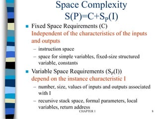
9. CHAPTER 1 9
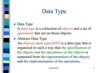
*Program 1.9: Simple arithmetic function (p.19)
float abc(float a, float b, float c)
{
return a + b + b * c + (a + b - c) / (a + b) + 4.00;
}
*Program 1.10: Iterative function for summing a list of numbers (p.20)
float sum(float list[ ], int n)
{
float tempsum = 0;
int i;
for (i = 0; i<n; i++)
tempsum += list [i];
return tempsum;
}
Sabc(I) = 0
Ssum(I) = 0
Recall: pass the address of the
first element of the array &
pass by value

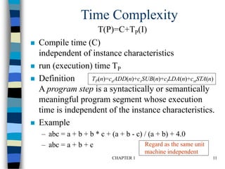
10. CHAPTER 1 10
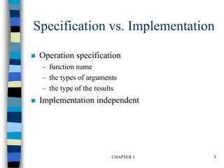
*Program 1.11: Recursive function for summing a list of numbers (p.20)
float rsum(float list[ ], int n)
{
if (n) return rsum(list, n-1) + list[n-1];
return 0;
}
*Figure 1.1: Space needed for one recursive call of Program 1.11 (p.21)
Type Name Number of bytes
parameter: float
parameter: integer
return address:(used internally)
list [ ]
n
2
2
2(unless a far address)
TOTAL per recursive call 6
Ssum(I)=Ssum(n)=6n
Assumptions:

11. CHAPTER 1 11
Time Complexity
 Compile time (C)
independent of instance characteristics
 run (execution) time TP
 Definition
A program step is a syntactically or semantically
meaningful program segment whose execution
time is independent of the instance characteristics.
 Example
– abc = a + b + b * c + (a + b - c) / (a + b) + 4.0
– abc = a + b + c Regard as the same unit
machine independent
T(P)=C+TP(I)
TP(n)=caADD(n)+csSUB(n)+clLDA(n)+cstSTA(n)

12. CHAPTER 1 12
Methods to compute the step count
 Introduce variable count into programs
 Tabular method
– Determine the total number of steps contributed by
each statement
step per execution  frequency
– add up the contribution of all statements

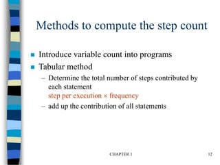
13. CHAPTER 1 13
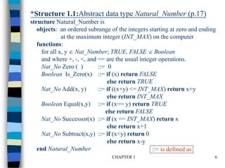
*Program 1.12: Program 1.10 with count statements (p.23)
float sum(float list[ ], int n)
{
float tempsum = 0; count++; /* for assignment */
int i;
for (i = 0; i < n; i++) {
count++; /*for the for loop */
tempsum += list[i]; count++; /* for assignment */
}
count++; /* last execution of for */
return tempsum;
count++; /* for return */
}
2n + 3 steps
Iterative summing of a list of numbers

14. CHAPTER 1 14
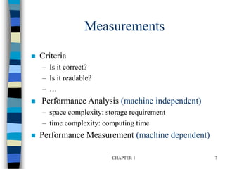
*Program 1.13: Simplified version of Program 1.12 (p.23)
float sum(float list[ ], int n)
{
float tempsum = 0;
int i;
for (i = 0; i < n; i++)
count += 2;
count += 3;
return 0;
}
2n + 3 steps

15. CHAPTER 1 15
*Program 1.14: Program 1.11 with count statements added (p.24)
float rsum(float list[ ], int n)
{
count++; /*for if conditional */
if (n) {
count++; /* for return and rsum invocation */
return rsum(list, n-1) + list[n-1];
}
count++;
return list[0];
}
2n+2
Recursive summing of a list of numbers

16. CHAPTER 1 16
*Program 1.15: Matrix addition (p.25)
void add( int a[ ] [MAX_SIZE], int b[ ] [MAX_SIZE],
int c [ ] [MAX_SIZE], int rows, int cols)
{
int i, j;
for (i = 0; i < rows; i++)
for (j= 0; j < cols; j++)
c[i][j] = a[i][j] +b[i][j];
}
Matrix addition

17. CHAPTER 1 17
*Program 1.16: Matrix addition with count statements (p.25)
void add(int a[ ][MAX_SIZE], int b[ ][MAX_SIZE],
int c[ ][MAX_SIZE], int row, int cols )
{
int i, j;
for (i = 0; i < rows; i++){
count++; /* for i for loop */
for (j = 0; j < cols; j++) {
count++; /* for j for loop */
c[i][j] = a[i][j] + b[i][j];
count++; /* for assignment statement */
}
count++; /* last time of j for loop */
}
count++; /* last time of i for loop */
}
2rows * cols + 2 rows + 1

18. CHAPTER 1 18
*Program 1.17: Simplification of Program 1.16 (p.26)
void add(int a[ ][MAX_SIZE], int b [ ][MAX_SIZE],
int c[ ][MAX_SIZE], int rows, int cols)
{
int i, j;
for( i = 0; i < rows; i++) {
for (j = 0; j < cols; j++)
count += 2;
count += 2;
}
count++;
}
2rows  cols + 2rows +1
Suggestion: Interchange the loops when rows >> cols

19. CHAPTER 1 19
*Figure 1.2: Step count table for Program 1.10 (p.26)
Statement s/e Frequency Total steps
float sum(float list[ ], int n)
{
float tempsum = 0;
int i;
for(i=0; i <n; i++)
tempsum += list[i];
return tempsum;
}
0 0 0
0 0 0
1 1 1
0 0 0
1 n+1 n+1
1 n n
1 1 1
0 0 0
Total 2n+3
Tabular Method
steps/execution
Iterative function to sum a list of numbers

20. CHAPTER 1 20
*Figure 1.3: Step count table for recursive summing function (p.27)
Statement s/e Frequency Total steps
float rsum(float list[ ], int n)
{
if (n)
return rsum(list, n-1)+list[n-1];
return list[0];
}
0 0 0
0 0 0
1 n+1 n+1
1 n n
1 1 1
0 0 0
Total 2n+2
Recursive Function to sum of a list of numbers

21. CHAPTER 1 21
*Figure 1.4: Step count table for matrix addition (p.27)
Statement s/e Frequency Total steps
Void add (int a[ ][MAX_SIZE]‧‧‧)
{
int i, j;
for (i = 0; i < row; i++)
for (j=0; j< cols; j++)
c[i][j] = a[i][j] + b[i][j];
}
0 0 0
0 0 0
0 0 0
1 rows+1 rows+1
1 rows‧(cols+1) rows‧cols+rows
1 rows‧cols rows‧cols
0 0 0
Total 2rows‧cols+2rows+1
Matrix Addition

22. CHAPTER 1 22
*Program 1.18: Printing out a matrix (p.28)
void print_matrix(int matrix[ ][MAX_SIZE], int rows, int cols)
{
int i, j;
for (i = 0; i < row; i++) {
for (j = 0; j < cols; j++)
printf(“%d”, matrix[i][j]);
printf( “n”);
}
}
Exercise 1

23. CHAPTER 1 23
*Program 1.19:Matrix multiplication function(p.28)
void mult(int a[ ][MAX_SIZE], int b[ ][MAX_SIZE], int c[ ][MAX_SIZE])
{
int i, j, k;
for (i = 0; i < MAX_SIZE; i++)
for (j = 0; j< MAX_SIZE; j++) {
c[i][j] = 0;
for (k = 0; k < MAX_SIZE; k++)
c[i][j] += a[i][k] * b[k][j];
}
}
Exercise 2

24. CHAPTER 1 24
*Program 1.20:Matrix product function(p.29)
void prod(int a[ ][MAX_SIZE], int b[ ][MAX_SIZE], int c[ ][MAX_SIZE],
int rowsa, int colsb, int colsa)
{
int i, j, k;
for (i = 0; i < rowsa; i++)
for (j = 0; j< colsb; j++) {
c[i][j] = 0;
for (k = 0; k< colsa; k++)
c[i][j] += a[i][k] * b[k][j];
}
}
Exercise 3

25. CHAPTER 1 25
*Program 1.21:Matrix transposition function (p.29)
void transpose(int a[ ][MAX_SIZE])
{
int i, j, temp;
for (i = 0; i < MAX_SIZE-1; i++)
for (j = i+1; j < MAX_SIZE; j++)
SWAP (a[i][j], a[j][i], temp);
}
Exercise 4

26. CHAPTER 1 26
Asymptotic Notation (O)
 Definition
f(n) = O(g(n)) iff there exist positive constants c
and n0 such that f(n)  cg(n) for all n, n  n0.
 Examples
– 3n+2=O(n) /* 3n+24n for n2 */
– 3n+3=O(n) /* 3n+34n for n3 */
– 100n+6=O(n) /* 100n+6101n for n10 */
– 10n2+4n+2=O(n2) /* 10n2+4n+211n2 for n5 */
– 6*2n+n2=O(2n) /* 6*2n+n2 7*2n for n4 */

27. CHAPTER 1 27
Example
 Complexity of c1n2+c2n and c3n
– for sufficiently large of value, c3n is faster than
c1n2+c2n
– for small values of n, either could be faster
• c1=1, c2=2, c3=100 --> c1n2+c2n  c3n for n  98
• c1=1, c2=2, c3=1000 --> c1n2+c2n  c3n for n  998
– break even point
• no matter what the values of c1, c2, and c3, the n
beyond which c3n is always faster than c1n2+c2n

28. CHAPTER 1 28
 O(1): constant
 O(n): linear
 O(n2): quadratic
 O(n3): cubic
 O(2n): exponential
 O(logn)
 O(nlogn)

29. CHAPTER 1 29
*Figure 1.7:Function values (p.38)

30. CHAPTER 1 30
*Figure 1.8:Plot of function values(p.39)
nlogn
n
logn

31. CHAPTER 1 31
*Figure 1.9:Times on a 1 billion instruction per second computer(p.40)