Download as PDF, PPTX


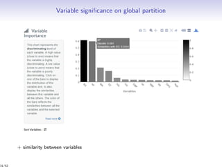
![Notations
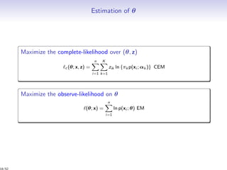
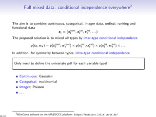
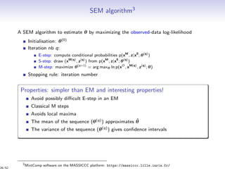
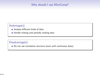
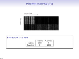
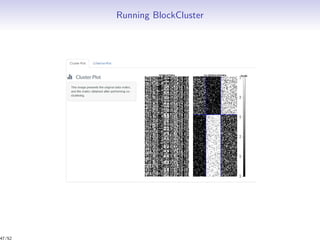
Data: n individuals: x = {x1, . . . , xn} = {xO , xM } in a space X of dimension d
Observed individuals xO
Missing individuals xM
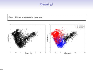
Aim: estimation of the partition z and the number of clusters K
Partition in K clusters G1, . . . , GK : z = (z1, . . . , zn), zi = (zi1, . . . , ziK )
xi ∈ Gk ⇔ zih = I{h=k}
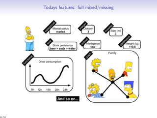
Mixed, missing, uncertain
Individuals x Partition z ⇔ Group
? 0.5 red 5 ? ? ? ⇔ ???
0.3 0.1 green 3 ? ? ? ⇔ ???
0.3 0.6 {red,green} 3 ? ? ? ⇔ ???
0.9 [0.25 0.45] red ? ? ? ? ⇔ ???
↓ ↓ ↓ ↓
continuous continuous categorical integer
12/52](https://image.slidesharecdn.com/presmassiccctechtalk-190529082243/85/Inria-Tech-Talk-La-classification-de-donnees-complexes-avec-MASSICCC-12-320.jpg)


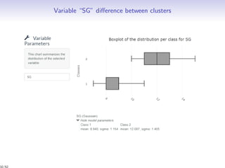

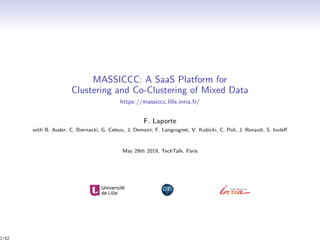
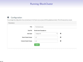
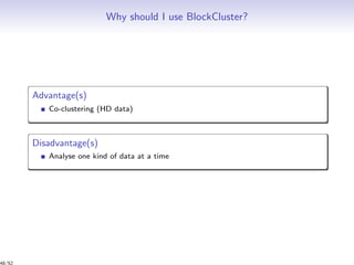
![From clustering to co-clustering
[Govaert, 2011]
38/52](https://image.slidesharecdn.com/presmassiccctechtalk-190529082243/85/Inria-Tech-Talk-La-classification-de-donnees-complexes-avec-MASSICCC-38-320.jpg)

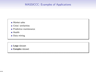
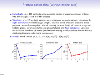
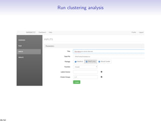
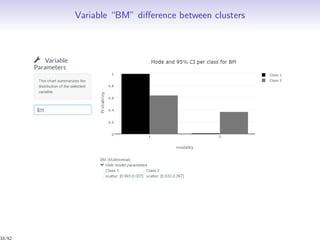
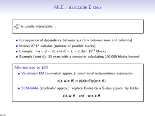
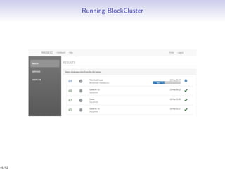
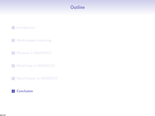
![MLE estimation: EM algorithm
Observed log-likelihood: (θ; x) = log p(x; θ)
Complete log-likelihood:
c (θ; x, z, w) = log p(x, z, w; θ)
=
i,k
zik log πk +
k,l
wjl log ρl +
i,j,k,l
zik wjl log p(xj
i ; αkl )
E-step of EM (iteration q):
Q(θ, θ(q)
) = E[ c (θ; x, z, w)|x; θ(q)
]
=
i,k
p(zi = k|x; θ(q)
)
t
(q)
ik
ln πk +
j,l
p(wi = l|x; θ(q)
)
s
(q)
jl
ln ρl
+
i,j,k,l
p(zi = k, wj = l|x; θ(q)
)
e
(q)
ijkl
ln p(xij ; αkl )
M-step of EM (iteration q): classical. For instance, for the Bernoulli case, it gives
π
(q+1)
k = i t
(q)
ik
n
, ρ
(q+1)
l =
j s
(q)
jl
d
, α
(q+1)
kl =
i,j e
(q)
ijkl xij
i,j e
(q)
ijkl
40/52](https://image.slidesharecdn.com/presmassiccctechtalk-190529082243/85/Inria-Tech-Talk-La-classification-de-donnees-complexes-avec-MASSICCC-40-320.jpg)


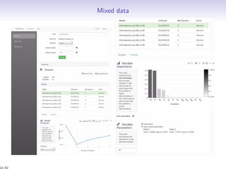
Massiccc is a software as a service (SaaS) platform designed for clustering and co-clustering of mixed data, catering to professionals and applications across various sectors such as predictive maintenance and health data mining. It offers advanced clustering techniques for dealing with complex datasets that include continuous, categorical, and missing data through various software modules like mixmod and mixtcomp. The platform aims to provide a user-friendly interface for analyzing large and intricate data sets while ensuring high-quality clustering results.