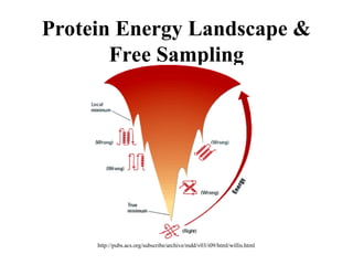
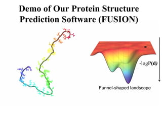
Protein Energy Landscape&
Free Sampling
http://pubs.acs.org/subscribe/archive/mdd/v03/i09/html/willis.html
4.
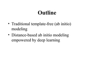
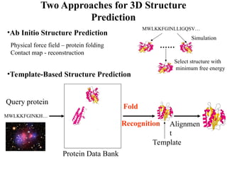
Two Approaches for3D Structure
Prediction
•Ab Initio Structure Prediction
•Template-Based Structure Prediction
Physical force field – protein folding
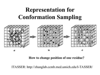
Contact map - reconstruction
MWLKKFGINLLIGQSV…
……
Select structure with
minimum free energy
MWLKKFGINKH…
Protein Data Bank
Fold
Recognition Alignmen
t
Template
Simulation
Query protein
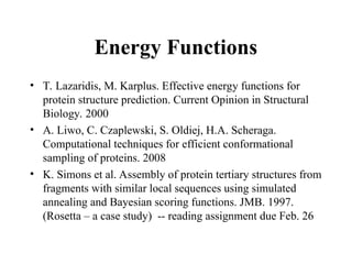
Energy Functions
• T.Lazaridis, M. Karplus. Effective energy functions for
protein structure prediction. Current Opinion in Structural
Biology. 2000
• A. Liwo, C. Czaplewski, S. Oldiej, H.A. Scheraga.
Computational techniques for efficient conformational
sampling of proteins. 2008
• K. Simons et al. Assembly of protein tertiary structures from
fragments with similar local sequences using simulated
annealing and Bayesian scoring functions. JMB. 1997.
(Rosetta – a case study) -- reading assignment due Feb. 26
8.
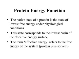
Protein Energy Function
•The native state of a protein is the state of
lowest free energy under physiological
conditions
• This state corresponds to the lowest basin of
the effective energy surface.
• The term ‘effective energy’ refers to the free
energy of the system (protein plus solvent)
9.
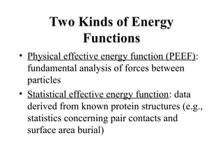
Two Kinds ofEnergy
Functions
• Physical effective energy function (PEEF):
fundamental analysis of forces between
particles
• Statistical effective energy function: data
derived from known protein structures (e.g.,
statistics concerning pair contacts and
surface area burial)
10.
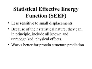
Statistical Effective Energy
Function(SEEF)
• Less sensitive to small displacements
• Because of their statistical nature, they can,
in principle, include all known and
unrecognized, physical effects.
• Works better for protein structure prediction
11.
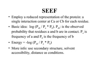
SEEF
• Employ areduced representation of the protein: a
single interaction center at Ca or Cb for each residue.
• Basic idea: log (Pab / Pa * Pb). Pab: is the observed
probability that residues a and b are in contact. Pa is
frequency of a and Pb is the frequency of b
• Energy = -log (Pab / Pa * Pb)
• More info: use secondary structure, solvent
accessibility, distance as conditions.
12.
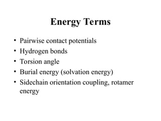
Energy Terms
• Pairwisecontact potentials
• Hydrogen bonds
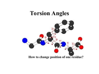
• Torsion angle
• Burial energy (solvation energy)
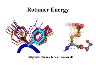
• Sidechain orientation coupling, rotamer
energy
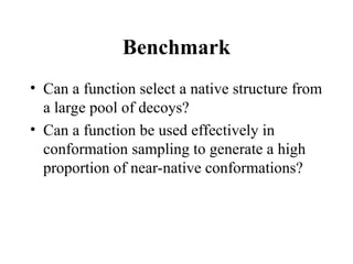
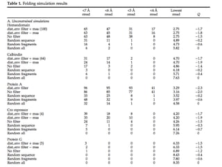
Benchmark
• Can afunction select a native structure from
a large pool of decoys?
• Can a function be used effectively in
conformation sampling to generate a high
proportion of near-native conformations?
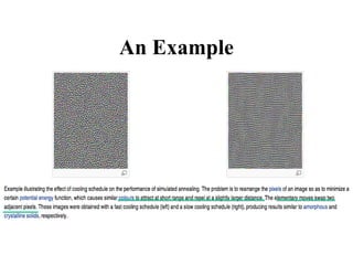
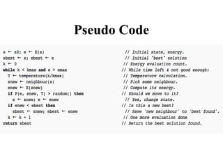
Simulated Annealing
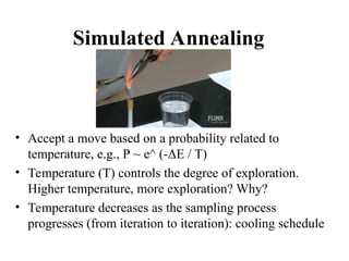
• Accepta move based on a probability related to
temperature, e.g., P ~ e^ (-ΔE / T)
• Temperature (T) controls the degree of exploration.
Higher temperature, more exploration? Why?
• Temperature decreases as the sampling process
progresses (from iteration to iteration): cooling schedule
A TFM Example:Rosetta
• K. Simons, C. Kooperberg, E. Huang, D.
Baker. Assembly of protein tertiary
structures from fragments with similar local
sequences using simulated annealing and
Bayesian scoring functions. JMB, 1997.
Rosetta: https://www.rosettacommons.org
23.
Basic Idea
• Shortsequence segments are restricted to
the local structures adopted by the most
closely related sequences in the PDB
• Use the observed local conformations of
similar local sequences to reduce sampling
space
24.
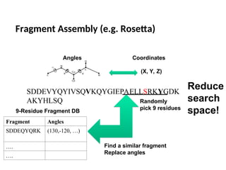
Fragment Assembly (e.g.Rosetta)
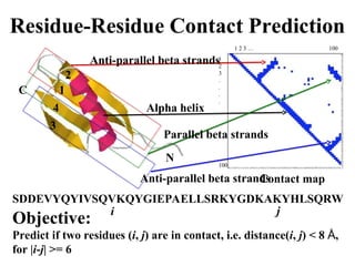
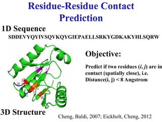
SDDEVYQYIVSQVKQYGIEPAELLSRKYGDK
AKYHLSQ
(X, Y, Z)
Angles Coordinates
Fragment Angles
SDDEQYQRK (130,-120, …)
….
….
9-Residue Fragment DB
Randomly
pick 9 residues
Find a similar fragment
Replace angles
Reduce
search
space!
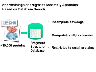
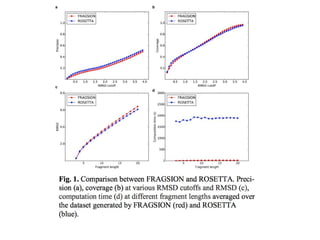
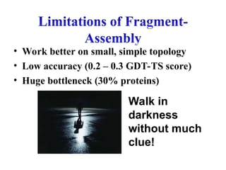
Shortcomings of FragmentAssembly Approach
Based on Database Search
• Computationally expensive
• Incomplete coverage
~80,000 proteins
• Restricted to small proteins
Fragment
Structure
Database
27.
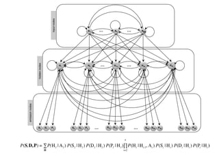
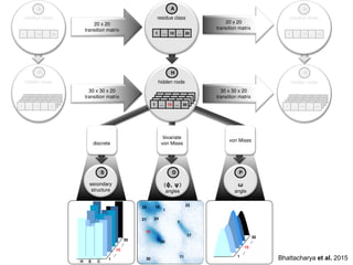
IOHMM (Input-Output Hidden
MarkovModel)
to model protein conformational space
Bhattacharya & Cheng, Bioinformatics, 2016
Bhattacharya & Cheng, Scientific Reports, 2015
hidden node
30 x30 x 20
transition matrix
30 x 30 x 20
transition matrix
residue class
1 … 10 … 20
discrete
bivariate
von Mises
von Mises
secondary
structure
(ϕ, ψ)
angles
ω
angle
1 … 15 … 30
hidden node
1 … 15 … 30
hidden node
1 … 15 … 30
20 x 20
transition matrix
20 x 20
transition matrix
residue class
1 … 10 … 20
residue class
1 … 10 … 20
H E C
1
17
20
25
30
24
1
…
15
30
…
1
…
15
30
…
21
11
19
7
15
23
Bhattacharya et al. 2015
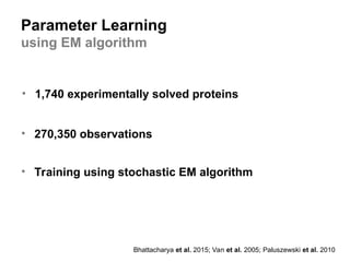
30.
Parameter Learning
using EMalgorithm
• 1,740 experimentally solved proteins
• 270,350 observations
• Training using stochastic EM algorithm
Bhattacharya et al. 2015; Van et al. 2005; Paluszewski et al. 2010
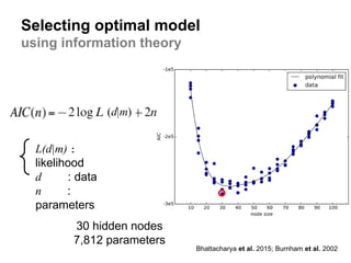
31.
Selecting optimal model
usinginformation theory
Bhattacharya et al. 2015; Burnham et al. 2002
L(d|m) :
likelihood
d : data
n :
parameters
30 hidden nodes
7,812 parameters
33.
Function of IOHMMModel of
Protein Conformation
• Sample the conformation of a (sub) sequence of any size
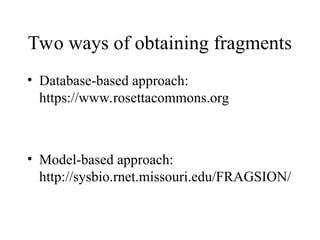
• Software: Fragsion:
http://sysbio.rnet.missouri.edu/FRAGSION/
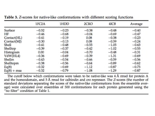
Scoring Functions ofSelecting
Local Conformations
• Knowledge-based potential functions
• Bayesian scoring function
One native assumption is P(structure) = 1 / # of structures.
36.
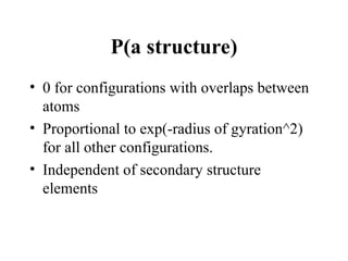
P(a structure)
• 0for configurations with overlaps between
atoms
• Proportional to exp(-radius of gyration^2)
for all other configurations.
• Independent of secondary structure
elements
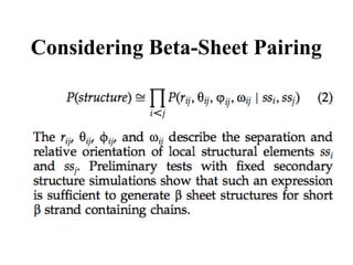
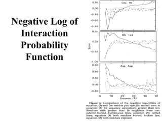
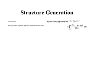
Scoring – P(Sequence|
Structure)
Ei can represent a variety of features of the local structural
environment around residue i.
(8)
40.
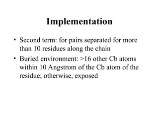
Implementation
• Second term:for pairs separated for more
than 10 residues along the chain
• Buried environment: >16 other Cb atoms
within 10 Angstrom of the Cb atom of the
residue; otherwise, exposed
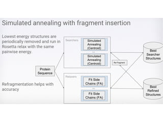
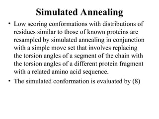
Simulated Annealing
• Lowscoring conformations with distributions of
residues similar to those of known proteins are
resampled by simulated annealing in conjunction
with a simple move set that involves replacing
the torsion angles of a segment of the chain with
the torsion angles of a different protein fragment
with a related amino acid sequence.
• The simulated conformation is evaluated by (8)
44.
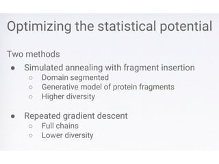
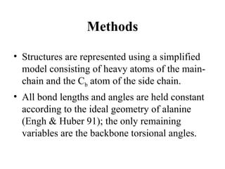
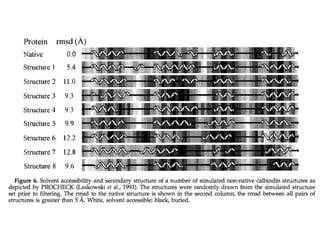
Methods
• Structures arerepresented using a simplified
model consisting of heavy atoms of the main-
chain and the Cb atom of the side chain.
• All bond lengths and angles are held constant
according to the ideal geometry of alanine
(Engh & Huber 91); the only remaining
variables are the backbone torsional angles.
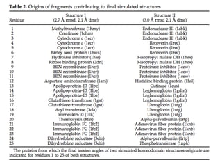
45.
Fragment Databases
• Nimers/ trimers (sequences) and their
conformations extracted from known
structures in the database
• Identify sequence neighbors: simple amino
acid frequency matching score.
46.
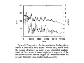
Simulation
• The startingconfiguration in all simulations was the fully extended chain.
• A move consists of substituting the torsional angles of a randomly chosen
neighbor at a randomly chosen position for those of the current
configuration.
• Moves which bring two atoms within 2.5 Angstrom are immediately
rejected; other moves are evaluated according to the Metropolis criterion
using the scoring equation.
• Simulated annealing was carried out by reducing the temperature from
2500 to 10 linearly over the course of 10,000 cycles (attempted moves).
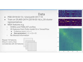
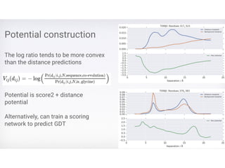
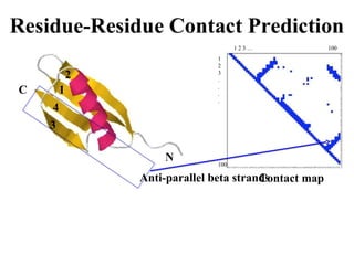
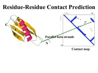
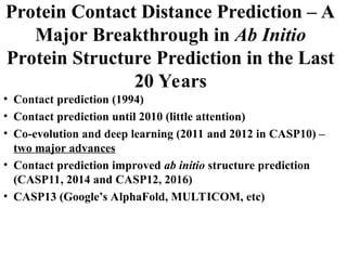
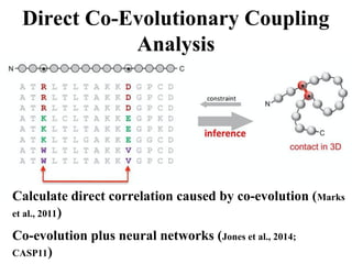
Protein Contact DistancePrediction – A
Major Breakthrough in Ab Initio
Protein Structure Prediction in the Last
20 Years
• Contact prediction (1994)
• Contact prediction until 2010 (little attention)
• Co-evolution and deep learning (2011 and 2012 in CASP10) –
two major advances
• Contact prediction improved ab initio structure prediction
(CASP11, 2014 and CASP12, 2016)
• CASP13 (Google’s AlphaFold, MULTICOM, etc)
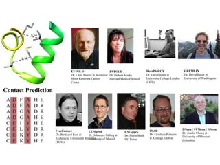
MetaPSICOV
Dr. David Jonesat
University College London
(UCL)
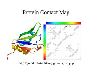
CMAppro
Dr. Pierre Baldi
UC Irvine
GREMLIN
Dr. David Baker at
University of Washington
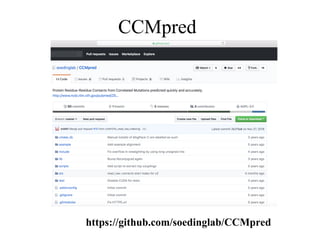
CCMpred
Dr. Johannes Söding at
University of Munich
FreeContact
Dr. Burkhard Rost at
Technische Universität München
(TUM)
DNcon / SVMcon / NNcon
Dr. Jianlin Cheng at
University of Missouri
Columbia
EVFOLD
Dr. Chris Sander at Memorial
Sloan Kettering Cancer
Center
EVFOLD
Dr. Debora Marks
Harvard Medical School
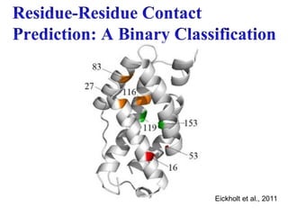
Contact Prediction
Distill
Dr. Gianluca Pollastri
U. College. Dublin
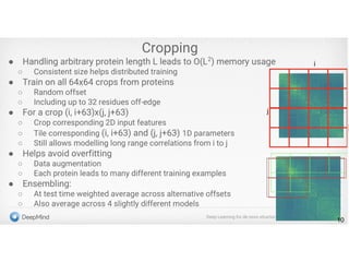
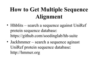
How to GetMultiple Sequence
Alignment
• Hhblits – search a sequence against UniRef
protein sequence database:
https://github.com/soedinglab/hh-suite
• Jackhmmer – search a sequence aginast
UniRef protein sequence database:
http://hmmer.org
Breakthrough II
• DeepLearning for Contact Prediction
(DNCON1) (Eickholt, Cheng, 2012)
• No. 1 in CASP10, 2012
• One of the first deep learning methods
for bioinformatics
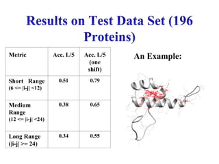
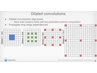
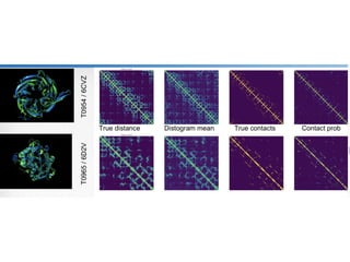
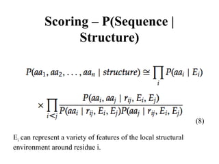
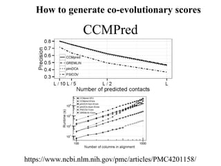
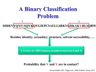
Accuracy of topL, L/5, or
L/10 predictions for various
ranges of sequence separation
(medium- and long-range):
[ TP/(TP+FP) ]
84.
Metric Acc. L/5Acc. L/5
(one
shift)
Short Range
(6 <= |i-j| <12)
0.51 0.79
Medium
Range
(12 <= |i-j| <24)
0.38 0.65
Long Range
(|i-j| >= 24)
0.34 0.55
An Example:
85.
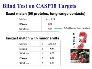
Method Acc. L/5
DNcon0.30
SVMcon 0.19
Method δ Acc. L/5
DNcon 1 0.53
SVMcon 1 0.37
DNcon 2 0.62
SVMcon 2 0.45
Exact match (96 proteins, long-range contacts)
Inexact match with minor shifts
9-fold better than random
86.
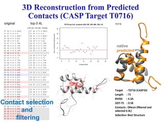
Target : T0716(CASP10)
Length : 71
RMSD : 4.3A
GDT-TS : 0.58
Contacts : DNcon (filtered and
selected 0.4L)
Selection: Best Structure
Contact selection
and
filtering
87.
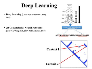
Deep Learning
• DeepLearning (CASP10; Eickholt and Cheng,
2012)
• 2D Convolutional Neural Networks
(CASP12; Wang et al., 2017; Adhikari et al., 2017)
Contact 1
Contact 2
88.
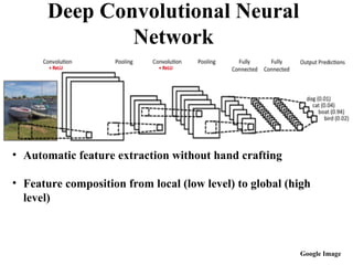
Deep Convolutional Neural
Network
•Automatic feature extraction without hand crafting
• Feature composition from local (low level) to global (high
level)
Google Image
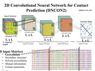
2D Convolutional NeuralNetwork for Contact
Prediction (DNCON2)
i j
• Co-evolution
• Secondary structure
• Solvent accessibility
• Mutual information
• Contact potentials
• …
D Input Matrices
Adhikari et al., 2017
L x L
L x L
L x L
L x L
L x L
L: sequence
length
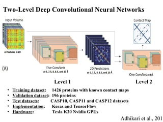
91.
Two-Level Deep ConvolutionalNeural Networks
• Training dataset: 1426 proteins with known contact maps
• Validation dataset: 196 proteins
• Test datasets: CASP10, CASP11 and CASP12 datasets
• Implementation: Keras and TensorFlow
• Hardware: Tesla K20 Nvidia GPUs
Adhikari et al., 2017
Level 1 Level 2
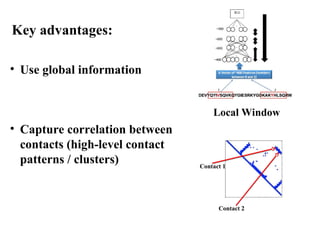
92.
• Use globalinformation
• Capture correlation between
contacts (high-level contact
patterns / clusters)
Local Window
Contact 1
Contact 2
Key advantages:
93.
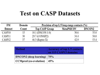
Test on CASPDatasets
Method Accuracy of top L/5 contacts
on 115 CASP13 domains
DNCON2 (deep learning) 75%
CCMpred (co-evolution) 45%
94.
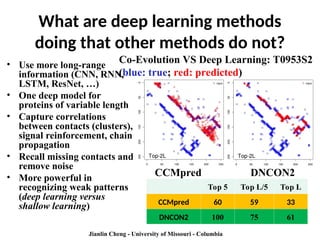
What are deeplearning methods
doing that other methods do not?
• Use more long-range
information (CNN, RNN,
LSTM, ResNet, …)
• One deep model for
proteins of variable length
• Capture correlations
between contacts (clusters),
signal reinforcement, chain
propagation
• Recall missing contacts and
remove noise
• More powerful in
recognizing weak patterns
(deep learning versus
shallow learning)
Top 5 Top L/5 Top L
CCMpred 60 59 33
DNCON2 100 75 61
Co-Evolution VS Deep Learning: T0953S2
(blue: true; red: predicted)
Jianlin Cheng - University of Missouri - Columbia
DNCON2
CCMpred
95.
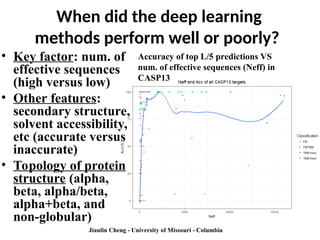
When did thedeep learning
methods perform well or poorly?
• Key factor: num. of
effective sequences
(high versus low)
• Other features:
secondary structure,
solvent accessibility,
etc (accurate versus
inaccurate)
• Topology of protein
structure (alpha,
beta, alpha/beta,
alpha+beta, and
non-globular)
Jianlin Cheng - University of Missouri - Columbia
Accuracy of top L/5 predictions VS
num. of effective sequences (Neff) in
CASP13
96.
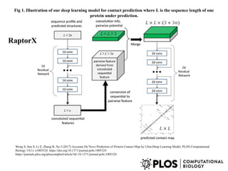
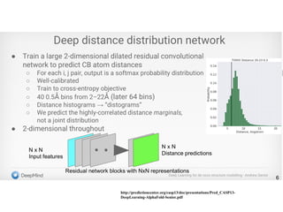
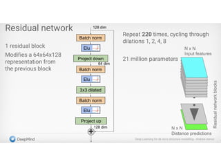
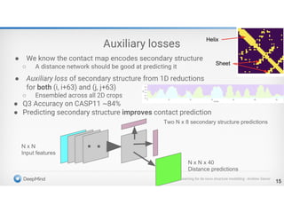
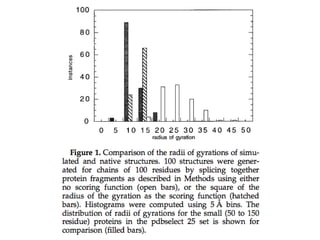
Fig 1. Illustrationof our deep learning model for contact prediction where L is the sequence length of one
protein under prediction.
Wang S, Sun S, Li Z, Zhang R, Xu J (2017) Accurate De Novo Prediction of Protein Contact Map by Ultra-Deep Learning Model. PLOS Computational
Biology 13(1): e1005324. https://doi.org/10.1371/journal.pcbi.1005324
https://journals.plos.org/ploscompbiol/article?id=10.1371/journal.pcbi.1005324
RaptorX
97.
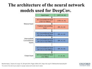
Bioinformatics, Volume 34,Issue 19, 26 April 2018, Pages 3308–3315, https://doi.org/10.1093/bioinformatics/bty341
The content of this slide may be subject to copyright: please see the slide notes for details.
The architecture of the neural network
models used for DeepCov.
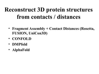
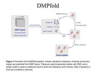
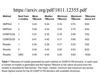
Reconstruct 3D proteinstructures
from contacts / distances
• Fragment Assembly + Contact Distances (Rosetta,
FUSION, UniCon3D)
• CONFOLD
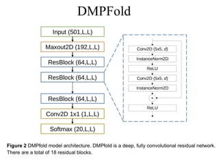
• DMPfold
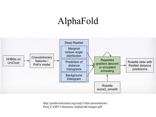
• AlphaFold
113.
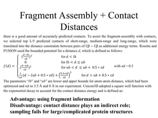
Fragment Assembly +Contact
Distances
Advantage: using fragment information
Disadvantage: contact distance plays an indirect role;
sampling fails for large/complicated protein structures
114.
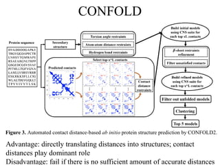
CONFOLD
Advantage: directly translatingdistances into structures; contact
distances play dominant role
Disadvantage: fail if there is no sufficient amount of accurate distances
115.
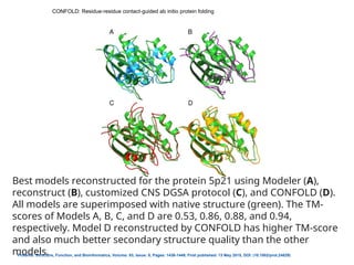
CONFOLD: Residue residuecontact guided ab initio protein folding
‐ ‐
Proteins: Structure, Function, and Bioinformatics, Volume: 83, Issue: 8, Pages: 1436-1449, First published: 13 May 2015, DOI: (10.1002/prot.24829)
Best models reconstructed for the protein 5p21 using Modeler (A),
reconstruct (B), customized CNS DGSA protocol (C), and CONFOLD (D).
All models are superimposed with native structure (green). The TM‐
scores of Models A, B, C, and D are 0.53, 0.86, 0.88, and 0.94,
respectively. Model D reconstructed by CONFOLD has higher TM‐score
and also much better secondary structure quality than the other
models.
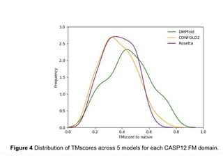
116.
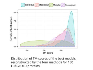
Distribution of TM‐scoresof the best models
reconstructed by the four methods for 150
FRAGFOLD proteins.
117.
CONFOLD VS EVFOLD
Bestpredicted models for the proteins RNH_ECOLI (A) and
SPTB2_HUMAN (B) using EVFOLD (purple) and CONFOLD
(orange) superimposed with native structures (green). The
TM‐scores of these models are reported in Table IV.
CONFOLD models have higher TM‐score and better
secondary structure quality than EVAFOLD.
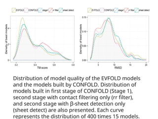
118.
Distribution of modelquality of the EVFOLD models
and the models built by CONFOLD. Distribution of
models built in first stage of CONFOLD (Stage 1),
second stage with contact filtering only (rr filter),
and second stage with β‐sheet detection only
(sheet detect) are also presented. Each curve
represents the distribution of 400 times 15 models.
119.
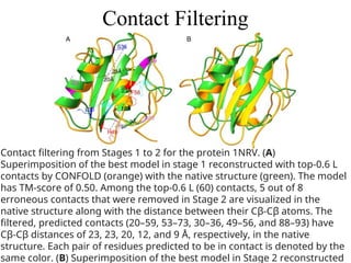
Contact Filtering
Contact filteringfrom Stages 1 to 2 for the protein 1NRV. (A)
Superimposition of the best model in stage 1 reconstructed with top‐0.6 L
contacts by CONFOLD (orange) with the native structure (green). The model
has TM‐score of 0.50. Among the top‐0.6 L (60) contacts, 5 out of 8
erroneous contacts that were removed in Stage 2 are visualized in the
native structure along with the distance between their Cβ‐Cβ atoms. The
filtered, predicted contacts (20–59, 53–73, 30–36, 49–56, and 88–93) have
Cβ‐Cβ distances of 23, 23, 20, 12, and 9 Å, respectively, in the native
structure. Each pair of residues predicted to be in contact is denoted by the
same color. (B) Superimposition of the best model in Stage 2 reconstructed
120.
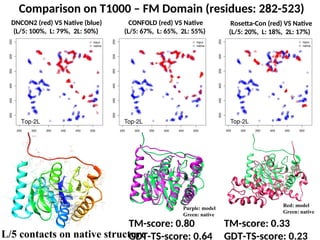
Comparison on T1000– FM Domain (residues: 282-523)
TM-score: 0.80
GDT-TS-score: 0.64
TM-score: 0.33
GDT-TS-score: 0.23
DNCON2 (red) VS Native (blue)
(L/5: 100%, L: 79%, 2L: 50%)
CONFOLD (red) VS Native
(L/5: 67%, L: 65%, 2L: 55%)
Rosetta-Con (red) VS Native
(L/5: 20%, L: 18%, 2L: 17%)
L/5 contacts on native structure
Purple: model
Green: native
Red: model
Green: native
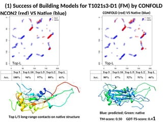
121.
(1) Success ofBuilding Models for T1021s3-D1 (FM) by CONFOLD
DNCON2 (red) VS Native (blue) CONFOLD (red) VS Native (blue)
Top L/5 long-range contacts on native structure
Blue: predicted; Green: native
TM-score: 0.50 GDT-TS-score: 0.41
Top 5 Top L/10 Top L/5 Top L/2 Top L
Acc. 100% 94% 97% 88% 61%
Top 5 Top L/10 Top L/5 Top L/2 Top L
Acc. 80% 47% 52% 51% 46%
122.
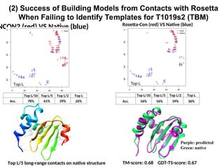
(2) Success ofBuilding Models from Contacts with Rosetta
When Failing to Identify Templates for T1019s2 (TBM)
TM-score: 0.68 GDT-TS-score: 0.67
Top L/5 long-range contacts on native structure
NCON2 (red) VS Native (blue) Rosetta-Con (red) VS Native (blue)
Top L/10 Top L/5 Top L/2 Top L
Acc. 78% 61% 39% 26%
Top L/10 Top L/5 Top L/2 Top L
Acc. 56% 56% 39% 36%
Purple: predicted
Green: native
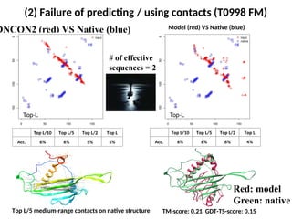
123.
(2) Failure ofpredicting / using contacts (T0998 FM)
Top L/10 Top L/5 Top L/2 Top L
Acc. 6% 6% 5% 5%
Top L/5 medium-range contacts on native structure
DNCON2 (red) VS Native (blue) Model (red) VS Native (blue)
# of effective
sequences = 2
TM-score: 0.21 GDT-TS-score: 0.15
Top L/10 Top L/5 Top L/2 Top L
Acc. 6% 6% 6% 4%
Red: model
Green: native
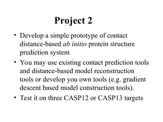
Project 2
• Developa simple prototype of contact
distance-based ab initio protein structure
prediction system
• You may use existing contact prediction tools
and distance-based model reconstruction
tools or develop you own tools (e.g. gradient
descent based model construction tools).
• Test it on three CASP12 or CASP13 targets
138.
Timeline
• March 18:discussion of the plan
• March 20: presentation of the plan
• April 3rd
, presentation of the results
• April 8th
, report due
139.
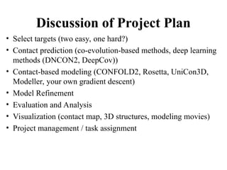
Discussion of ProjectPlan
• Select targets (two easy, one hard?)
• Contact prediction (co-evolution-based methods, deep learning
methods (DNCON2, DeepCov))
• Contact-based modeling (CONFOLD2, Rosetta, UniCon3D,
Modeller, your own gradient descent)
• Model Refinement
• Evaluation and Analysis
• Visualization (contact map, 3D structures, modeling movies)
• Project management / task assignment
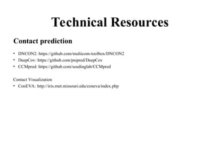
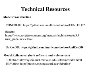
Technical Resources
Model reconstruction
ModelRefinement (both software and web servers)
CONFOLD2: https://github.com/multicom-toolbox/CONFOLD2
Rosetta:
https://www.rosettacommons.org/manuals/archive/rosetta3.4_
user_guide/index.html
UniCon3D: https://github.com/multicom-toolbox/UniCon3D
i3DRefine: http://protein.rnet.missouri.edu/i3drefine/
3DRefine: http://sysbio.rnet.missouri.edu/3Drefine/index.html
Editor's Notes
#28 glycines, prolines, β-branched residues isoleucine and valine, most frequently encountered ‘generic’ class, and each of these groups preceding prolines.
#68 amount of effort currently being spent to improve contact prediction accuracy
#86 Contact Filtering: Contact filtering was applied to predicted DNcon contacts. Contacts were divided into Long Range (LR), Short Range (SR), and Medium Range (MR). From each of these groups top contacts were selected to make the top 0.4L contacts.
The grey structure with red lines shows the predicted structure and the contacts used to fold the structure.
#112 We consider each region of genome as a bead and the entire genome is a string of beads. Then we place those beads in 3D such that the distances between beads are consistent with the 2D contact map.
#115 Best models reconstructed for the protein 5p21 using Modeler (A), reconstruct (B), customized CNS DGSA protocol (C), and CONFOLD (D). All models are superimposed with native structure (green). The TM‐scores of Models A, B, C, and D are 0.53, 0.86, 0.88, and 0.94, respectively. Model D reconstructed by CONFOLD has higher TM‐score and also much better secondary structure quality than the other models.
IF THIS IMAGE HAS BEEN PROVIDED BY OR IS OWNED BY A THIRD PARTY, AS INDICATED IN THE CAPTION LINE, THEN FURTHER PERMISSION MAY BE NEEDED BEFORE ANY FURTHER USE. PLEASE CONTACT WILEY'S PERMISSIONS DEPARTMENT ON PERMISSIONS@WILEY.COM OR USE THE RIGHTSLINK SERVICE BY CLICKING ON THE 'REQUEST PERMISSIONS' LINK ACCOMPANYING THIS ARTICLE. WILEY OR AUTHOR OWNED IMAGES MAY BE USED FOR NON-COMMERCIAL PURPOSES, SUBJECT TO PROPER CITATION OF THE ARTICLE, AUTHOR, AND PUBLISHER.


![…
…
…
…
…
…
…
[0,1]
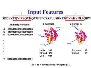
1239 Proteins for Training
Residue Pairs (|i-j| >= 6)](https://image.slidesharecdn.com/3proteintfm2019-250324085851-064cdbc0/85/Template-Free-Protein-Structure-Modeling-79-320.jpg)
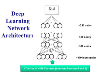
![Speed up training by
CUDAMat and GPUs
Train DNs with over 1M
parameters in about an
hour
…
…
…
…
…
…
[0,1]
…
LSDEKIINVDF KPSEERVREII](https://image.slidesharecdn.com/3proteintfm2019-250324085851-064cdbc0/85/Template-Free-Protein-Structure-Modeling-80-320.jpg)
![…
…
…
…
…
…
[0,1]
…
…
…
…
…
…
…
[0,1]
…
…
…
…
…
…
…
[0,1]
…
……
[0,1]
Final output of ensemble
is a performance weighted
sum of individual DN
outputs.
Eickholt and Cheng, Bioinformatics (2012)](https://image.slidesharecdn.com/3proteintfm2019-250324085851-064cdbc0/85/Template-Free-Protein-Structure-Modeling-81-320.jpg)
![…
…
…
…
…
…
[0,1]
…
…
…
…
…
…
…
[0,1]
…
…
…
…
…
…
…
[0,1]
…
……
[0,1]
Final output of ensemble
is a performance weighted
sum of individual DN
outputs.
Eickholt and Cheng, Bioinformatics (2012)](https://image.slidesharecdn.com/3proteintfm2019-250324085851-064cdbc0/85/Template-Free-Protein-Structure-Modeling-82-320.jpg)
![Accuracy of top L, L/5, or
L/10 predictions for various
ranges of sequence separation
(medium- and long-range):
[ TP/(TP+FP) ]](https://image.slidesharecdn.com/3proteintfm2019-250324085851-064cdbc0/85/Template-Free-Protein-Structure-Modeling-83-320.jpg)