Download free for 30 days
Sign in
Upload
Language (EN)
Support
Business
Mobile
Social Media
Marketing
Technology
Art & Photos
Career
Design
Education
Presentations & Public Speaking
Government & Nonprofit
Healthcare
Internet
Law
Leadership & Management
Automotive
Engineering
Software
Recruiting & HR
Retail
Sales
Services
Science
Small Business & Entrepreneurship
Food
Environment
Economy & Finance
Data & Analytics
Investor Relations
Sports
Spiritual
News & Politics
Travel
Self Improvement
Real Estate
Entertainment & Humor
Health & Medicine
Devices & Hardware
Lifestyle
Change Language
Language
English
Español
Português
Français
Deutsche
Cancel
Save
Submit search
EN
Uploaded by
seaiteccoop
PPTX, PDF
61 views
Ch02 Probability Concepts and Applications.pptx
Ch02 Probability Concepts and Applications.pptx
Education
◦
Read more
0
Save
Share
Embed
Embed presentation
Download
Download to read offline
1
/ 99
2
/ 99
Most read
3
/ 99
4
/ 99
5
/ 99
6
/ 99
7
/ 99
8
/ 99
Most read
9
/ 99
10
/ 99
11
/ 99
12
/ 99
13
/ 99
14
/ 99
Most read
15
/ 99
16
/ 99
17
/ 99
18
/ 99
19
/ 99
20
/ 99
21
/ 99
22
/ 99
23
/ 99
24
/ 99
25
/ 99
26
/ 99
27
/ 99
28
/ 99
29
/ 99
30
/ 99
31
/ 99
32
/ 99
33
/ 99
34
/ 99
35
/ 99
36
/ 99
37
/ 99
38
/ 99
39
/ 99
40
/ 99
41
/ 99
42
/ 99
43
/ 99
44
/ 99
45
/ 99
46
/ 99
47
/ 99
48
/ 99
49
/ 99
50
/ 99
51
/ 99
52
/ 99
53
/ 99
54
/ 99
55
/ 99
56
/ 99
57
/ 99
58
/ 99
59
/ 99
60
/ 99
61
/ 99
62
/ 99
63
/ 99
64
/ 99
65
/ 99
66
/ 99
67
/ 99
68
/ 99
69
/ 99
70
/ 99
71
/ 99
72
/ 99
73
/ 99
74
/ 99
75
/ 99
76
/ 99
77
/ 99
78
/ 99
79
/ 99
80
/ 99
81
/ 99
82
/ 99
83
/ 99
84
/ 99
85
/ 99
86
/ 99
87
/ 99
88
/ 99
89
/ 99
90
/ 99
91
/ 99
92
/ 99
93
/ 99
94
/ 99
95
/ 99
96
/ 99
97
/ 99
98
/ 99
99
/ 99
More Related Content
PPTX
Class PPT About Quantitative Business Analysis
by
MiqdadRobbani3
PDF
PPT Teching The Cass about the Quantitative
by
MiqdadRobbani3
PPTX
Bba 3274 qm week 2 probability concepts
by
Stephen Ong
PPT
Rsh qam11 ch02
by
Firas Husseini
PPT
Probability concepts-applications-1235015791722176-2
by
satysun1990
PPT
Probability Concepts Applications
by
guest44b78
PPTX
Statistical Analysis with R -II
by
Akhila Prabhakaran
PPTX
probability-120611030603-phpapp02.pptx
by
SoujanyaLk1
Class PPT About Quantitative Business Analysis
by
MiqdadRobbani3
PPT Teching The Cass about the Quantitative
by
MiqdadRobbani3
Bba 3274 qm week 2 probability concepts
by
Stephen Ong
Rsh qam11 ch02
by
Firas Husseini
Probability concepts-applications-1235015791722176-2
by
satysun1990
Probability Concepts Applications
by
guest44b78
Statistical Analysis with R -II
by
Akhila Prabhakaran
probability-120611030603-phpapp02.pptx
by
SoujanyaLk1
Similar to Ch02 Probability Concepts and Applications.pptx
PPTX
UNIT I_StatisticsandProbability1234.pptx
by
pritimalkhede
PPT
Probability concepts and procedures law of profitability
by
kamalsapkota13
PPTX
Probability basics and bayes' theorem
by
Balaji P
PDF
Probability Theory MSc BA Sem 2.pdf
by
ssuserd329601
PPT
PROBABILITY AND IT'S TYPES WITH RULES
by
Bhargavi Bhanu
PPT
Statistics: Probability
by
Sultan Mahmood
KEY
Probability Review
by
Tomoki Tsuchida
PPTX
Class 11 Basic Probability.pptx
by
CallplanetsDeveloper
PPTX
Concept of probability_Dr. NL(23-1-23).pptx
by
Anaes6
PPTX
Probability
by
Mahi Muthananickal
PPTX
Probability
by
Rushina Singhi
PPTX
Probability and probability distribution.pptx
by
abubekeremam245
PPTX
introduction of probabilityChapter5.pptx
by
epheremabera12345
PPTX
Probability & probability distribution
by
umar sheikh
PPTX
Claas 11 Basic Probability.pptx
by
CallplanetsDeveloper
PPTX
Introduction of Probability
by
rey castro
PDF
chap03--Discrete random variables probability ai and ml R2021.pdf
by
mitopof121
PPTX
Probabilty1.pptx
by
KemalAbdela2
PPTX
Discussion of Simple and Compound Probability
by
NormanAReyes
PPTX
L1-Fundamentals of Probability. gives fundamentals of statistics and probabil...
by
NishthaShah16
UNIT I_StatisticsandProbability1234.pptx
by
pritimalkhede
Probability concepts and procedures law of profitability
by
kamalsapkota13
Probability basics and bayes' theorem
by
Balaji P
Probability Theory MSc BA Sem 2.pdf
by
ssuserd329601
PROBABILITY AND IT'S TYPES WITH RULES
by
Bhargavi Bhanu
Statistics: Probability
by
Sultan Mahmood
Probability Review
by
Tomoki Tsuchida
Class 11 Basic Probability.pptx
by
CallplanetsDeveloper
Concept of probability_Dr. NL(23-1-23).pptx
by
Anaes6
Probability
by
Mahi Muthananickal
Probability
by
Rushina Singhi
Probability and probability distribution.pptx
by
abubekeremam245
introduction of probabilityChapter5.pptx
by
epheremabera12345
Probability & probability distribution
by
umar sheikh
Claas 11 Basic Probability.pptx
by
CallplanetsDeveloper
Introduction of Probability
by
rey castro
chap03--Discrete random variables probability ai and ml R2021.pdf
by
mitopof121
Probabilty1.pptx
by
KemalAbdela2
Discussion of Simple and Compound Probability
by
NormanAReyes
L1-Fundamentals of Probability. gives fundamentals of statistics and probabil...
by
NishthaShah16
Recently uploaded
PPTX
Weaving Threads: Mapping Practitioner Theses to Understand Professional Becom...
by
Samuel Mann
PPTX
INSTRUCTIONAL MATERIALS IN TEACHING SCIENCE.pptx
by
ReclaMailyn1
PDF
RPT FORM 1 English (2026 academic session) SMKTS.pdf
by
WANAHMADAZIMIBINWANA
PDF
BÀI GIẢNG POWERPOINT CHÍNH KHÓA PHIÊN BẢN AI TIẾNG ANH 6 CẢ NĂM, THEO TỪNG BÀ...
by
Nguyen Thanh Tu Collection
PPTX
bundle of care.pptx Priti Bala @ BRD med
by
pritibala13
PPTX
How to Manage Empty Location in Odoo 18 Inventory
by
Celine George
PPTX
RECTAL IRRIGATION...................pptx
by
AneetaSharma15
PDF
Geography unit 7-Population-Distribution`.pdf
by
zerihunbrook7
PPTX
VITAMINS CHAPTER NO.05 PHARMACOGNOSY D. PHARMACY
by
Ganu Gavade
PDF
GIÁO ÁN KẾ HOẠCH BÀI DẠY NĂNG LỰC SỐ MÔN TIẾNG ANH LỚP 10 CẢ NĂM - GLOBAL SUC...
by
Nguyen Thanh Tu Collection
PPTX
Nanomaterials and its types - Dr.M.Jothimuniyandi
by
Jothimuniyandi
PPTX
Exploring car engine oil and lubricants purpose and functions
by
mjb77ny
PDF
GIÁO ÁN KẾ HOẠCH BÀI DẠY NĂNG LỰC SỐ MÔN TIẾNG ANH LỚP 12 CẢ NĂM - GLOBAL SUC...
by
Nguyen Thanh Tu Collection
PPTX
The Creation Pattern Physical Health.pptx
by
Tammy Hulse
PPTX
Activity on Job position in Odoo 19 Recruitment
by
Celine George
PPTX
How to Manage Scheduling Activities in Odoo 18 CRM
by
Celine George
DOCX
COMMUNITY HEALTH NURSING OSCE CHECKLIST.docx
by
Geetha S R
PDF
BÀI GIẢNG POWERPOINT CHÍNH KHÓA PHIÊN BẢN AI TIẾNG ANH 6 CẢ NĂM, THEO TỪNG BÀ...
by
Nguyen Thanh Tu Collection
PDF
Problem Solving Agents in Artificial Intelligence with Examples and Water Jug...
by
ARTHIDEVARANIP
PDF
To synthesis and submit Benzamide synthesis.pdf
by
Pradeep Swarnkar
Weaving Threads: Mapping Practitioner Theses to Understand Professional Becom...
by
Samuel Mann
INSTRUCTIONAL MATERIALS IN TEACHING SCIENCE.pptx
by
ReclaMailyn1
RPT FORM 1 English (2026 academic session) SMKTS.pdf
by
WANAHMADAZIMIBINWANA
BÀI GIẢNG POWERPOINT CHÍNH KHÓA PHIÊN BẢN AI TIẾNG ANH 6 CẢ NĂM, THEO TỪNG BÀ...
by
Nguyen Thanh Tu Collection
bundle of care.pptx Priti Bala @ BRD med
by
pritibala13
How to Manage Empty Location in Odoo 18 Inventory
by
Celine George
RECTAL IRRIGATION...................pptx
by
AneetaSharma15
Geography unit 7-Population-Distribution`.pdf
by
zerihunbrook7
VITAMINS CHAPTER NO.05 PHARMACOGNOSY D. PHARMACY
by
Ganu Gavade
GIÁO ÁN KẾ HOẠCH BÀI DẠY NĂNG LỰC SỐ MÔN TIẾNG ANH LỚP 10 CẢ NĂM - GLOBAL SUC...
by
Nguyen Thanh Tu Collection
Nanomaterials and its types - Dr.M.Jothimuniyandi
by
Jothimuniyandi
Exploring car engine oil and lubricants purpose and functions
by
mjb77ny
GIÁO ÁN KẾ HOẠCH BÀI DẠY NĂNG LỰC SỐ MÔN TIẾNG ANH LỚP 12 CẢ NĂM - GLOBAL SUC...
by
Nguyen Thanh Tu Collection
The Creation Pattern Physical Health.pptx
by
Tammy Hulse
Activity on Job position in Odoo 19 Recruitment
by
Celine George
How to Manage Scheduling Activities in Odoo 18 CRM
by
Celine George
COMMUNITY HEALTH NURSING OSCE CHECKLIST.docx
by
Geetha S R
BÀI GIẢNG POWERPOINT CHÍNH KHÓA PHIÊN BẢN AI TIẾNG ANH 6 CẢ NĂM, THEO TỪNG BÀ...
by
Nguyen Thanh Tu Collection
Problem Solving Agents in Artificial Intelligence with Examples and Water Jug...
by
ARTHIDEVARANIP
To synthesis and submit Benzamide synthesis.pdf
by
Pradeep Swarnkar
Ch02 Probability Concepts and Applications.pptx
1.
Chapter 2 To accompany Quantitative
Analysis for Management, Eleventh Edition, by Render, Stair, and Hanna Power Point slides created by Brian Peterson Probability Concepts and Applications
2.
Copyright ©2012 Pearson
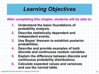
Education, Inc. publishing as Prentice Hall 2-2 Learning Objectives 1. Understand the basic foundations of probability analysis. 2. Describe statistically dependent and independent events. 3. Use Bayes’ theorem to establish posterior probabilities. 4. Describe and provide examples of both discrete and continuous random variables. 5. Explain the difference between discrete and continuous probability distributions. 6. Calculate expected values and variances and use the normal table. After completing this chapter, students will be able to:
3.
Copyright ©2012 Pearson
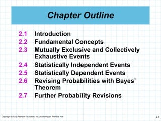
Education, Inc. publishing as Prentice Hall 2-3 Chapter Outline 2.1 Introduction 2.2 Fundamental Concepts 2.3 Mutually Exclusive and Collectively Exhaustive Events 2.4 Statistically Independent Events 2.5 Statistically Dependent Events 2.6 Revising Probabilities with Bayes’ Theorem 2.7 Further Probability Revisions
4.
Copyright ©2012 Pearson
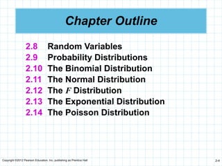
Education, Inc. publishing as Prentice Hall 2-4 Chapter Outline 2.8 Random Variables 2.9 Probability Distributions 2.10 The Binomial Distribution 2.11 The Normal Distribution 2.12 The F Distribution 2.13 The Exponential Distribution 2.14 The Poisson Distribution
5.
Copyright ©2012 Pearson
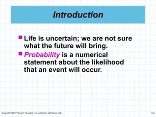
Education, Inc. publishing as Prentice Hall 2-5 Introduction Life is uncertain; we are not sure what the future will bring. Probability is a numerical statement about the likelihood that an event will occur.
6.
Copyright ©2012 Pearson
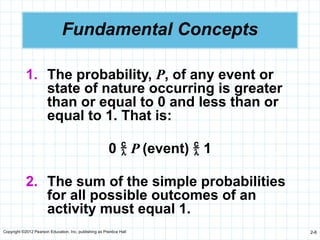
Education, Inc. publishing as Prentice Hall 2-6 Fundamental Concepts 1. The probability, P, of any event or state of nature occurring is greater than or equal to 0 and less than or equal to 1. That is: 0 P (event) 1 2. The sum of the simple probabilities for all possible outcomes of an activity must equal 1.
7.
Copyright ©2012 Pearson
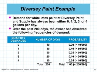
Education, Inc. publishing as Prentice Hall 2-7 Diversey Paint Example Demand for white latex paint at Diversey Paint and Supply has always been either 0, 1, 2, 3, or 4 gallons per day. Over the past 200 days, the owner has observed the following frequencies of demand: QUANTITY DEMANDED NUMBER OF DAYS PROBABILITY 0 40 0.20 (= 40/200) 1 80 0.40 (= 80/200) 2 50 0.25 (= 50/200) 3 20 0.10 (= 20/200) 4 10 0.05 (= 10/200) Total 200 Total 1.00 (= 200/200)
8.
Copyright ©2012 Pearson
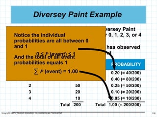
Education, Inc. publishing as Prentice Hall 2-8 Diversey Paint Example Demand for white latex paint at Diversey Paint and Supply has always been either 0, 1, 2, 3, or 4 gallons per day Over the past 200 days, the owner has observed the following frequencies of demand QUANTITY DEMANDED NUMBER OF DAYS PROBABILITY 0 40 0.20 (= 40/200) 1 80 0.40 (= 80/200) 2 50 0.25 (= 50/200) 3 20 0.10 (= 20/200) 4 10 0.05 (= 10/200) Total 200 Total 1.00 (= 200/200) Notice the individual probabilities are all between 0 and 1 0 ≤ P (event) ≤ 1 And the total of all event probabilities equals 1 ∑ P (event) = 1.00
9.
Copyright ©2012 Pearson
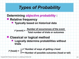
Education, Inc. publishing as Prentice Hall 2-9 Determining objective probability : Relative frequency Typically based on historical data Types of Probability P (event) = Number of occurrences of the event Total number of trials or outcomes Classical or logical method Logically determine probabilities without trials P (head) = 1 2 Number of ways of getting a head Number of possible outcomes (head or tail)
10.
Copyright ©2012 Pearson
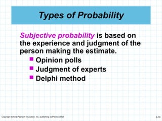
Education, Inc. publishing as Prentice Hall 2-10 Types of Probability Subjective probability is based on the experience and judgment of the person making the estimate. Opinion polls Judgment of experts Delphi method
11.
Copyright ©2012 Pearson
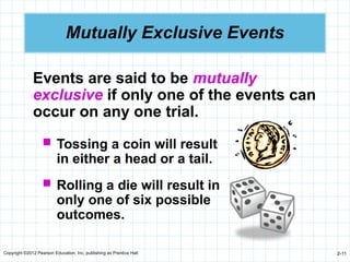
Education, Inc. publishing as Prentice Hall 2-11 Mutually Exclusive Events Events are said to be mutually exclusive if only one of the events can occur on any one trial. Tossing a coin will result in either a head or a tail. Rolling a die will result in only one of six possible outcomes.
12.
Copyright ©2012 Pearson
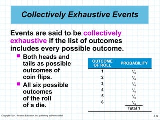
Education, Inc. publishing as Prentice Hall 2-12 Collectively Exhaustive Events Events are said to be collectively exhaustive if the list of outcomes includes every possible outcome. Both heads and tails as possible outcomes of coin flips. All six possible outcomes of the roll of a die. OUTCOME OF ROLL PROBABILITY 1 1 /6 2 1 /6 3 1 /6 4 1 /6 5 1 /6 6 1 /6 Total 1
13.
Copyright ©2012 Pearson
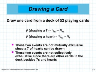
Education, Inc. publishing as Prentice Hall 2-13 Drawing a Card Draw one card from a deck of 52 playing cards P (drawing a 7) = 4 /52 = 1 /13 P (drawing a heart) = 13 /52 = 1 /4 These two events are not mutually exclusive since a 7 of hearts can be drawn These two events are not collectively exhaustive since there are other cards in the deck besides 7s and hearts
14.
Copyright ©2012 Pearson
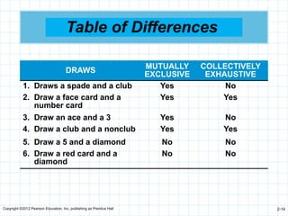
Education, Inc. publishing as Prentice Hall 2-14 Table of Differences DRAWS MUTUALLY EXCLUSIVE COLLECTIVELY EXHAUSTIVE 1. Draws a spade and a club Yes No 2. Draw a face card and a number card Yes Yes 3. Draw an ace and a 3 Yes No 4. Draw a club and a nonclub Yes Yes 5. Draw a 5 and a diamond No No 6. Draw a red card and a diamond No No
15.
Copyright ©2012 Pearson
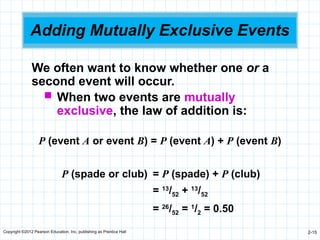
Education, Inc. publishing as Prentice Hall 2-15 Adding Mutually Exclusive Events We often want to know whether one or a second event will occur. When two events are mutually exclusive, the law of addition is: P (event A or event B) = P (event A) + P (event B) P (spade or club) = P (spade) + P (club) = 13 /52 + 13 /52 = 26 /52 = 1 /2 = 0.50
16.
Copyright ©2012 Pearson
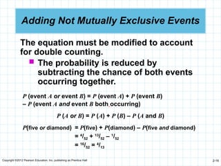
Education, Inc. publishing as Prentice Hall 2-16 Adding Not Mutually Exclusive Events P (event A or event B) = P (event A) + P (event B) – P (event A and event B both occurring) P (A or B) = P (A) + P (B) – P (A and B) P(five or diamond) = P(five) + P(diamond) – P(five and diamond) = 4 /52 + 13 /52 – 1 /52 = 16 /52 = 4 /13 The equation must be modified to account for double counting. The probability is reduced by subtracting the chance of both events occurring together.
17.
Copyright ©2012 Pearson
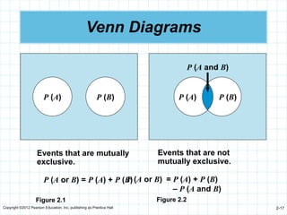
Education, Inc. publishing as Prentice Hall 2-17 Venn Diagrams P (A) P (B) Events that are mutually exclusive. P (A or B) = P (A) + P (B) Figure 2.1 Events that are not mutually exclusive. P (A or B) = P (A) + P (B) – P (A and B) Figure 2.2 P (A) P (B) P (A and B)
18.
Copyright ©2012 Pearson
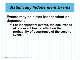
Education, Inc. publishing as Prentice Hall 2-18 Statistically Independent Events Events may be either independent or dependent. For independent events, the occurrence of one event has no effect on the probability of occurrence of the second event.
19.
Copyright ©2012 Pearson
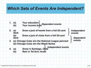
Education, Inc. publishing as Prentice Hall 2-19 Which Sets of Events Are Independent? 1. (a) Your education (b) Your income level 2. (a) Draw a jack of hearts from a full 52-card deck (b) Draw a jack of clubs from a full 52-card deck 3. (a) Chicago Cubs win the National League pennant (b) Chicago Cubs win the World Series 4. (a) Snow in Santiago, Chile (b) Rain in Tel Aviv, Israel Dependent events Dependent events Independent events Independent events
20.
Copyright ©2012 Pearson
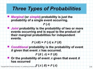
Education, Inc. publishing as Prentice Hall 2-20 Three Types of Probabilities Marginal (or simple) probability is just the probability of a single event occurring. P (A) Joint probability is the probability of two or more events occurring and is equal to the product of their marginal probabilities for independent events. P (AB) = P (A) x P (B) Conditional probability is the probability of event B given that event A has occurred. P (B | A) = P (B) Or the probability of event A given that event B has occurred P (A | B) = P (A)
21.
Copyright ©2012 Pearson
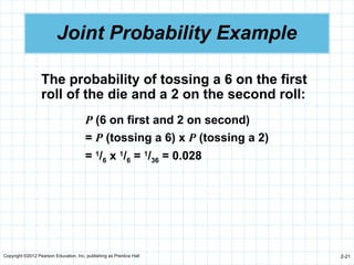
Education, Inc. publishing as Prentice Hall 2-21 Joint Probability Example The probability of tossing a 6 on the first roll of the die and a 2 on the second roll: P (6 on first and 2 on second) = P (tossing a 6) x P (tossing a 2) = 1 /6 x 1 /6 = 1 /36 = 0.028
22.
Copyright ©2012 Pearson
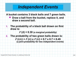
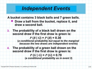
Education, Inc. publishing as Prentice Hall 2-22 Independent Events 1. The probability of a black ball drawn on first draw is: P (B) = 0.30 (a marginal probability) 2. The probability of two green balls drawn is: P (GG) = P (G) x P (G) = 0.7 x 0.7 = 0.49 (a joint probability for two independent events) A bucket contains 3 black balls and 7 green balls. Draw a ball from the bucket, replace it, and draw a second ball.
23.
Copyright ©2012 Pearson
Education, Inc. publishing as Prentice Hall 2-23 Independent Events 3. The probability of a black ball drawn on the second draw if the first draw is green is: P (B | G) = P (B) = 0.30 (a conditional probability but equal to the marginal because the two draws are independent events) 4. The probability of a green ball drawn on the second draw if the first draw is green is: P (G | G) = P (G) = 0.70 (a conditional probability as in event 3) A bucket contains 3 black balls and 7 green balls. Draw a ball from the bucket, replace it, and draw a second ball.
24.
Copyright ©2012 Pearson
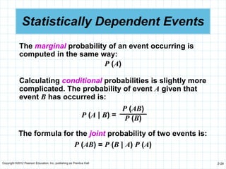
Education, Inc. publishing as Prentice Hall 2-24 Statistically Dependent Events The marginal probability of an event occurring is computed in the same way: P (A) The formula for the joint probability of two events is: P (AB) = P (B | A) P (A) P (A | B) = P (AB) P (B) Calculating conditional probabilities is slightly more complicated. The probability of event A given that event B has occurred is:
25.
Copyright ©2012 Pearson
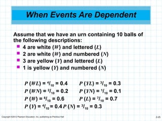
Education, Inc. publishing as Prentice Hall 2-25 When Events Are Dependent Assume that we have an urn containing 10 balls of the following descriptions: 4 are white (W) and lettered (L) 2 are white (W) and numbered (N) 3 are yellow (Y) and lettered (L) 1 is yellow (Y) and numbered (N) P (WL) = 4 /10 = 0.4 P (YL) = 3 /10 = 0.3 P (WN) = 2 /10 = 0.2 P (YN) = 1 /10 = 0.1 P (W) = 6 /10 = 0.6 P (L) = 7 /10 = 0.7 P (Y) = 4 /10 = 0.4P (N) = 3 /10 = 0.3
26.
Copyright ©2012 Pearson
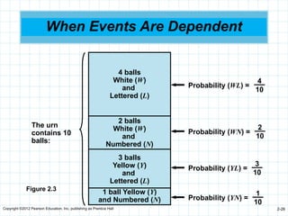
Education, Inc. publishing as Prentice Hall 2-26 When Events Are Dependent 4 balls White (W) and Lettered (L) 2 balls White (W) and Numbered (N) 3 balls Yellow (Y) and Lettered (L) 1 ball Yellow (Y) and Numbered (N) Probability (WL) = 4 10 Probability (YN) = 1 10 Probability (YL) = 3 10 Probability (WN) = 2 10 The urn contains 10 balls: Figure 2.3
27.
Copyright ©2012 Pearson
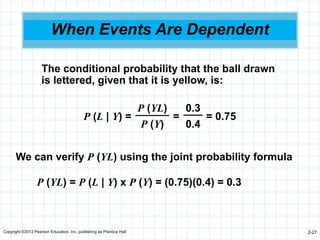
Education, Inc. publishing as Prentice Hall 2-27 When Events Are Dependent The conditional probability that the ball drawn is lettered, given that it is yellow, is: P (L | Y) = = = 0.75 P (YL) P (Y) 0.3 0.4 We can verify P (YL) using the joint probability formula P (YL) = P (L | Y) x P (Y) = (0.75)(0.4) = 0.3
28.
Copyright ©2012 Pearson
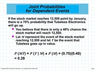
Education, Inc. publishing as Prentice Hall 2-28 Joint Probabilities for Dependent Events P (MT) = P (T | M) x P (M) = (0.70)(0.40) = 0.28 If the stock market reaches 12,500 point by January, there is a 70% probability that Tubeless Electronics will go up. You believe that there is only a 40% chance the stock market will reach 12,500. Let M represent the event of the stock market reaching 12,500 and let T be the event that Tubeless goes up in value.
29.
Copyright ©2012 Pearson
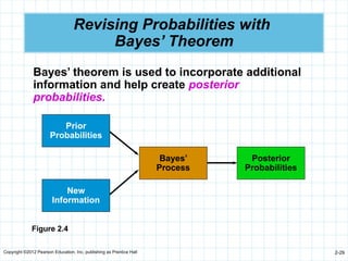
Education, Inc. publishing as Prentice Hall 2-29 Posterior Probabilities Bayes’ Process Revising Probabilities with Bayes’ Theorem Bayes’ theorem is used to incorporate additional information and help create posterior probabilities. Prior Probabilities New Information Figure 2.4
30.
Copyright ©2012 Pearson
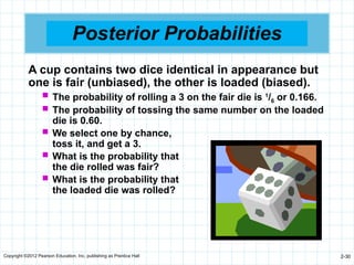
Education, Inc. publishing as Prentice Hall 2-30 Posterior Probabilities A cup contains two dice identical in appearance but one is fair (unbiased), the other is loaded (biased). The probability of rolling a 3 on the fair die is 1 /6 or 0.166. The probability of tossing the same number on the loaded die is 0.60. We select one by chance, toss it, and get a 3. What is the probability that the die rolled was fair? What is the probability that the loaded die was rolled?
31.
Copyright ©2012 Pearson
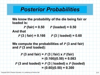
Education, Inc. publishing as Prentice Hall 2-31 Posterior Probabilities We know the probability of the die being fair or loaded is: P (fair) = 0.50 P (loaded) = 0.50 And that P (3 | fair) = 0.166 P (3 | loaded) = 0.60 We compute the probabilities of P (3 and fair) and P (3 and loaded): P (3 and fair) = P (3 | fair) x P (fair) = (0.166)(0.50) = 0.083 P (3 and loaded) = P (3 | loaded) x P (loaded) = (0.60)(0.50) = 0.300
32.
Copyright ©2012 Pearson
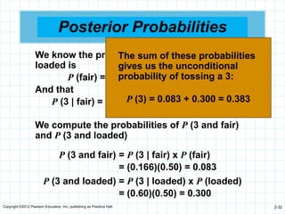
Education, Inc. publishing as Prentice Hall 2-32 Posterior Probabilities We know the probability of the die being fair or loaded is P (fair) = 0.50 P (loaded) = 0.50 And that P (3 | fair) = 0.166 P (3 | loaded) = 0.60 We compute the probabilities of P (3 and fair) and P (3 and loaded) P (3 and fair) = P (3 | fair) x P (fair) = (0.166)(0.50) = 0.083 P (3 and loaded) = P (3 | loaded) x P (loaded) = (0.60)(0.50) = 0.300 The sum of these probabilities gives us the unconditional probability of tossing a 3: P (3) = 0.083 + 0.300 = 0.383
33.
Copyright ©2012 Pearson
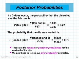
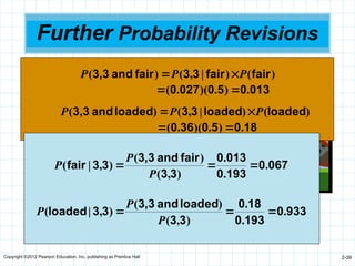
Education, Inc. publishing as Prentice Hall 2-33 Posterior Probabilities P (loaded | 3) = = = 0.78 P (loaded and 3) P (3) 0.300 0.383 The probability that the die was loaded is: P (fair | 3) = = = 0.22 P (fair and 3) P (3) 0.083 0.383 If a 3 does occur, the probability that the die rolled was the fair one is: These are the revised or posterior probabilities for the next roll of the die. We use these to revise our prior probability estimates.
34.
Copyright ©2012 Pearson
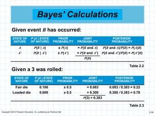
Education, Inc. publishing as Prentice Hall 2-34 Bayes’ Calculations Given event B has occurred: STATE OF NATURE P (B | STATE OF NATURE) PRIOR PROBABILITY JOINT PROBABILITY POSTERIOR PROBABILITY A P(B | A) x P(A) = P(B and A) P(B and A)/P(B) = P(A|B) A’ P(B | A’) x P(A’) = P(B and A’) P(B and A’)/P(B) = P(A’|B) P(B) Table 2.2 Given a 3 was rolled: STATE OF NATURE P (B | STATE OF NATURE) PRIOR PROBABILITY JOINT PROBABILITY POSTERIOR PROBABILITY Fair die 0.166 x 0.5 = 0.083 0.083 / 0.383 = 0.22 Loaded die 0.600 x 0.5 = 0.300 0.300 / 0.383 = 0.78 P(3) = 0.383 Table 2.3
35.
Copyright ©2012 Pearson
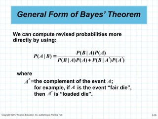
Education, Inc. publishing as Prentice Hall 2-35 General Form of Bayes’ Theorem ) ( ) | ( ) ( ) | ( ) ( ) | ( ) | ( A P A B P A P A B P A P A B P B A P We can compute revised probabilities more directly by using: where the complement of the event ; for example, if is the event “fair die”, then is “loaded die”. A A A = ¢ A
36.
Copyright ©2012 Pearson
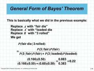
Education, Inc. publishing as Prentice Hall 2-36 General Form of Bayes’ Theorem This is basically what we did in the previous example: Replace with “fair die” Replace with “loaded die Replace with “3 rolled” We get A A B ) | ( rolled 3 die fair P ) ( ) | ( ) ( ) | ( ) ( ) | ( loaded loaded 3 fair fair 3 fair fair 3 P P P P P P 22 0 383 0 083 0 50 0 60 0 50 0 166 0 50 0 166 0 . . . ) . )( . ( ) . )( . ( ) . )( . (
37.
Copyright ©2012 Pearson
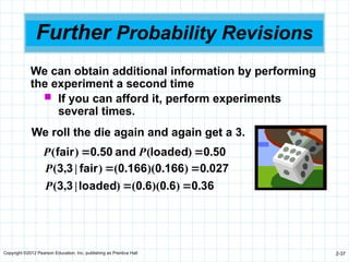
Education, Inc. publishing as Prentice Hall 2-37 Further Probability Revisions We can obtain additional information by performing the experiment a second time If you can afford it, perform experiments several times. We roll the die again and again get a 3. 50 0 loaded and 50 0 fair . ) ( . ) ( P P 36 0 6 0 6 0 loaded 3 3 027 0 166 0 166 0 fair 3 3 . ) . )( . ( ) | , ( . ) . )( . ( ) | , ( P P
38.
Copyright ©2012 Pearson
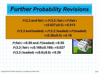
Education, Inc. publishing as Prentice Hall 2-38 Further Probability Revisions We can obtain additional information by performing the experiment a second time If you can afford it, perform experiments several times We roll the die again and again get a 3 50 0 loaded and 50 0 fair . ) ( . ) ( P P 36 0 6 0 6 0 loaded 3 3 027 0 166 0 166 0 fair 3 3 . ) . )( . ( ) | , ( . ) . )( . ( ) | , ( P P ) ( ) | , ( ) ( fair fair 3 3 fair and 3,3 P P P 013 0 5 0 027 0 . ) . )( . ( ) ( ) | , ( ) ( loaded loaded 3 3 loaded and 3,3 P P P 18 0 5 0 36 0 . ) . )( . (
39.
Copyright ©2012 Pearson
Education, Inc. publishing as Prentice Hall 2-39 Further Probability Revisions We can obtain additional information by performing the experiment a second time If you can afford it, perform experiments several times We roll the die again and again get a 3 50 . 0 ) loaded ( and 50 . 0 ) fair ( P P 36 . 0 ) 6 . 0 )( 6 . 0 ( ) loaded | 3 , 3 ( 027 . 0 ) 166 . 0 )( 166 . 0 ( ) fair | 3 , 3 ( P P ) ( ) | , ( ) ( fair fair 3 3 fair and 3,3 P P P 013 0 5 0 027 0 . ) . )( . ( ) ( ) | , ( ) ( loaded loaded 3 3 loaded and 3,3 P P P 18 0 5 0 36 0 . ) . )( . ( 067 0 193 0 013 0 3 3 fair and 3,3 3 3 fair . . . ) , ( ) ( ) , | ( P P P 933 0 193 0 18 0 3 3 loaded and 3,3 3 3 loaded . . . ) , ( ) ( ) , | ( P P P
40.
Copyright ©2012 Pearson
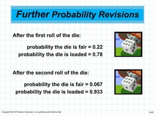
Education, Inc. publishing as Prentice Hall 2-40 Further Probability Revisions After the first roll of the die: probability the die is fair = 0.22 probability the die is loaded = 0.78 After the second roll of the die: probability the die is fair = 0.067 probability the die is loaded = 0.933
41.
Copyright ©2012 Pearson
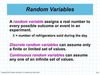
Education, Inc. publishing as Prentice Hall 2-41 Random Variables Discrete random variables can assume only a finite or limited set of values. Continuous random variables can assume any one of an infinite set of values. A random variable assigns a real number to every possible outcome or event in an experiment. X = number of refrigerators sold during the day
42.
Copyright ©2012 Pearson
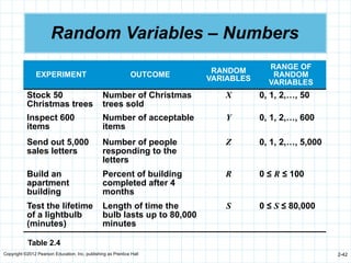
Education, Inc. publishing as Prentice Hall 2-42 Random Variables – Numbers EXPERIMENT OUTCOME RANDOM VARIABLES RANGE OF RANDOM VARIABLES Stock 50 Christmas trees Number of Christmas trees sold X 0, 1, 2,…, 50 Inspect 600 items Number of acceptable items Y 0, 1, 2,…, 600 Send out 5,000 sales letters Number of people responding to the letters Z 0, 1, 2,…, 5,000 Build an apartment building Percent of building completed after 4 months R 0 ≤ R ≤ 100 Test the lifetime of a lightbulb (minutes) Length of time the bulb lasts up to 80,000 minutes S 0 ≤ S ≤ 80,000 Table 2.4
43.
Copyright ©2012 Pearson
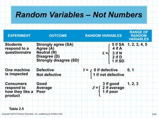
Education, Inc. publishing as Prentice Hall 2-43 Random Variables – Not Numbers EXPERIMENT OUTCOME RANDOM VARIABLES RANGE OF RANDOM VARIABLES Students respond to a questionnaire Strongly agree (SA) Agree (A) Neutral (N) Disagree (D) Strongly disagree (SD) 5 if SA 4 if A.. X = 3 if N.. 2 if D.. 1 if SD 1, 2, 3, 4, 5 One machine is inspected Defective Not defective Y = 0 if defective 1 if not defective 0, 1 Consumers respond to how they like a product Good Average Poor 3 if good…. Z = 2 if average 1 if poor….. 1, 2, 3 Table 2.5
44.
Copyright ©2012 Pearson
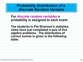
Education, Inc. publishing as Prentice Hall 2-44 Probability Distribution of a Discrete Random Variable The students in Pat Shannon’s statistics class have just completed a quiz of five algebra problems. The distribution of correct scores is given in the following table: For discrete random variables a probability is assigned to each event.
45.
Copyright ©2012 Pearson
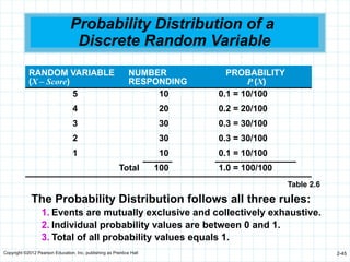
Education, Inc. publishing as Prentice Hall 2-45 Probability Distribution of a Discrete Random Variable RANDOM VARIABLE (X – Score) NUMBER RESPONDING PROBABILITY P (X) 5 10 0.1 = 10/100 4 20 0.2 = 20/100 3 30 0.3 = 30/100 2 30 0.3 = 30/100 1 10 0.1 = 10/100 Total 100 1.0 = 100/100 The Probability Distribution follows all three rules: 1. Events are mutually exclusive and collectively exhaustive. 2. Individual probability values are between 0 and 1. 3. Total of all probability values equals 1. Table 2.6
46.
Copyright ©2012 Pearson
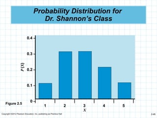
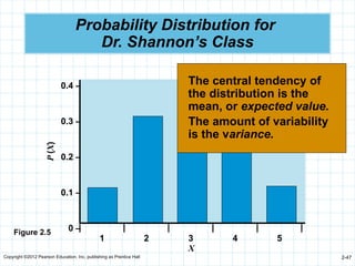
Education, Inc. publishing as Prentice Hall 2-46 Probability Distribution for Dr. Shannon’s Class P (X) 0.4 – 0.3 – 0.2 – 0.1 – 0 – | | | | | | 1 2 3 4 5 X Figure 2.5
47.
Copyright ©2012 Pearson
Education, Inc. publishing as Prentice Hall 2-47 Probability Distribution for Dr. Shannon’s Class P (X) 0.4 – 0.3 – 0.2 – 0.1 – 0 – | | | | | | 1 2 3 4 5 X Figure 2.5 The central tendency of the distribution is the mean, or expected value. The amount of variability is the variance.
48.
Copyright ©2012 Pearson
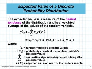
Education, Inc. publishing as Prentice Hall 2-48 Expected Value of a Discrete Probability Distribution n i i i X P X X E 1 ) ( ... ) ( 2 2 1 1 n n X P X X P X X P X The expected value is a measure of the central tendency of the distribution and is a weighted average of the values of the random variable. where i X ) ( i X P n i 1 ) (X E = random variable’s possible values = probability of each of the random variable’s possible values = summation sign indicating we are adding all n possible values = expected value or mean of the random sample
49.
Copyright ©2012 Pearson
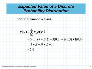
Education, Inc. publishing as Prentice Hall 2-49 Expected Value of a Discrete Probability Distribution n i i i X P X X E 1 9 . 2 1 . 6 . 9 . 8 . 5 . ) 1 . 0 ( 1 ) 3 . 0 ( 2 ) 3 . 0 ( 3 ) 2 . 0 ( 4 ) 1 . 0 ( 5 For Dr. Shannon’s class:
50.
Copyright ©2012 Pearson
Education, Inc. publishing as Prentice Hall 2-50 Variance of a Discrete Probability Distribution For a discrete probability distribution the variance can be computed by ) ( )] ( [ n i i i X P X E X 1 2 2 Variance σ where i X ) (X E ) ( i X P = random variable’s possible values = expected value of the random variable = difference between each value of the random variable and the expected mean = probability of each possible value of the random variable )] ( [ X E Xi
51.
Copyright ©2012 Pearson
Education, Inc. publishing as Prentice Hall 2-51 Variance of a Discrete Probability Distribution For Dr. Shannon’s class: ) ( )] ( [ variance 5 1 2 i i i X P X E X ) . ( ) . ( ) . ( ) . ( variance 2 0 9 2 4 1 0 9 2 5 2 2 ) . ( ) . ( ) . ( ) . ( 3 0 9 2 2 3 0 9 2 3 2 2 ) . ( ) . ( 1 0 9 2 1 2 29 1 361 0 243 0 003 0 242 0 441 0 . . . . . .
52.
Copyright ©2012 Pearson
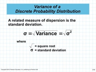
Education, Inc. publishing as Prentice Hall 2-52 Variance of a Discrete Probability Distribution A related measure of dispersion is the standard deviation. 2 σ Variance σ where σ = square root = standard deviation
53.
Copyright ©2012 Pearson
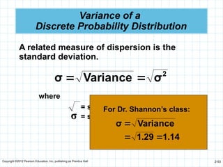
Education, Inc. publishing as Prentice Hall 2-53 Variance of a Discrete Probability Distribution A related measure of dispersion is the standard deviation. 2 σ Variance σ where σ = square root = standard deviation For Dr. Shannon’s class: Variance σ 14 1 29 1 . .
54.
Copyright ©2012 Pearson
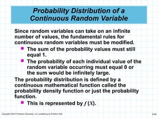
Education, Inc. publishing as Prentice Hall 2-54 Probability Distribution of a Continuous Random Variable Since random variables can take on an infinite number of values, the fundamental rules for continuous random variables must be modified. The sum of the probability values must still equal 1. The probability of each individual value of the random variable occurring must equal 0 or the sum would be infinitely large. The probability distribution is defined by a continuous mathematical function called the probability density function or just the probability function. This is represented by f (X).
55.
Copyright ©2012 Pearson
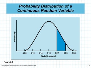
Education, Inc. publishing as Prentice Hall 2-55 Probability Distribution of a Continuous Random Variable Probability | | | | | | | 5.06 5.10 5.14 5.18 5.22 5.26 5.30 Weight (grams) Figure 2.6
56.
Copyright ©2012 Pearson
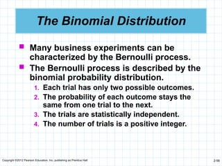
Education, Inc. publishing as Prentice Hall 2-56 The Binomial Distribution Many business experiments can be characterized by the Bernoulli process. The Bernoulli process is described by the binomial probability distribution. 1. Each trial has only two possible outcomes. 2. The probability of each outcome stays the same from one trial to the next. 3. The trials are statistically independent. 4. The number of trials is a positive integer.
57.
Copyright ©2012 Pearson
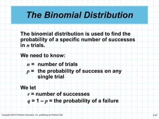
Education, Inc. publishing as Prentice Hall 2-57 The Binomial Distribution The binomial distribution is used to find the probability of a specific number of successes in n trials. We need to know: n = number of trials p = the probability of success on any single trial We let r = number of successes q = 1 – p = the probability of a failure
58.
Copyright ©2012 Pearson
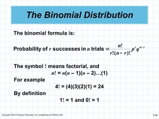
Education, Inc. publishing as Prentice Hall 2-58 The Binomial Distribution The binomial formula is: r n r q p r n r n n r )! ( ! ! trials in successes of y Probabilit The symbol ! means factorial, and n! = n(n – 1)(n – 2)…(1) For example 4! = (4)(3)(2)(1) = 24 By definition 1! = 1 and 0! = 1
59.
Copyright ©2012 Pearson
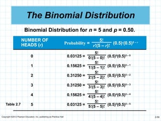
Education, Inc. publishing as Prentice Hall 2-59 The Binomial Distribution NUMBER OF HEADS (r) Probability = (0.5)r (0.5)5 – r 5! r!(5 – r)! 0 0.03125 = (0.5)0 (0.5)5 – 0 1 0.15625 = (0.5)1 (0.5)5 – 1 2 0.31250 = (0.5)2 (0.5)5 – 2 3 0.31250 = (0.5)3 (0.5)5 – 3 4 0.15625 = (0.5)4 (0.5)5 – 4 5 0.03125 = (0.5)5 (0.5)5 – 5 5! 0!(5 – 0)! 5! 1!(5 – 1)! 5! 2!(5 – 2)! 5! 3!(5 – 3)! 5! 4!(5 – 4)! 5! 5!(5 – 5)! Table 2.7 Binomial Distribution for n = 5 and p = 0.50.
60.
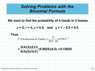
Copyright ©2012 Pearson
Education, Inc. publishing as Prentice Hall 2-60 Solving Problems with the Binomial Formula We want to find the probability of 4 heads in 5 tosses. n = 5, r = 4, p = 0.5, and q = 1 – 0.5 = 0.5 Thus 4 5 4 5 . 0 5 . 0 )! 4 5 ( ! 4 ! 5 ) trials 5 in successes 4 ( P 15625 0 5 0 0625 0 1 1 2 3 4 1 2 3 4 5 . ) . )( . ( ) ! )( )( )( ( ) )( )( )( (
61.
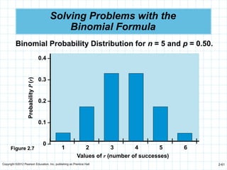
Copyright ©2012 Pearson
Education, Inc. publishing as Prentice Hall 2-61 Solving Problems with the Binomial Formula Probability P (r) | | | | | | | 1 2 3 4 5 6 Values of r (number of successes) 0.4 – 0.3 – 0.2 – 0.1 – 0 – Figure 2.7 Binomial Probability Distribution for n = 5 and p = 0.50.
62.
Copyright ©2012 Pearson
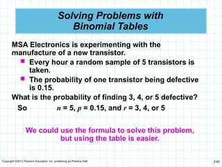
Education, Inc. publishing as Prentice Hall 2-62 Solving Problems with Binomial Tables MSA Electronics is experimenting with the manufacture of a new transistor. Every hour a random sample of 5 transistors is taken. The probability of one transistor being defective is 0.15. What is the probability of finding 3, 4, or 5 defective? n = 5, p = 0.15, and r = 3, 4, or 5 So We could use the formula to solve this problem, but using the table is easier.
63.
Copyright ©2012 Pearson
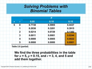
Education, Inc. publishing as Prentice Hall 2-63 Solving Problems with Binomial Tables P n r 0.05 0.10 0.15 5 0 0.7738 0.5905 0.4437 1 0.2036 0.3281 0.3915 2 0.0214 0.0729 0.1382 3 0.0011 0.0081 0.0244 4 0.0000 0.0005 0.0022 5 0.0000 0.0000 0.0001 Table 2.8 (partial) We find the three probabilities in the table for n = 5, p = 0.15, and r = 3, 4, and 5 and add them together.
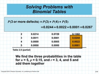
64.
Copyright ©2012 Pearson
Education, Inc. publishing as Prentice Hall 2-64 Table 2.8 (partial) We find the three probabilities in the table for n = 5, p = 0.15, and r = 3, 4, and 5 and add them together Solving Problems with Binomial Tables P n r 0.05 0.10 0.15 5 0 0.7738 0.5905 0.4437 1 0.2036 0.3281 0.3915 2 0.0214 0.0729 0.1382 3 0.0011 0.0081 0.0244 4 0.0000 0.0005 0.0022 5 0.0000 0.0000 0.0001 ) ( ) ( ) ( ) ( 5 4 3 defects more or 3 P P P P 0267 0 0001 0 0022 0 0244 0 . . . .
65.
Copyright ©2012 Pearson
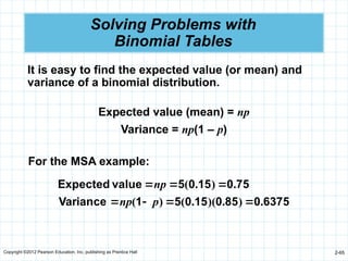
Education, Inc. publishing as Prentice Hall 2-65 Solving Problems with Binomial Tables It is easy to find the expected value (or mean) and variance of a binomial distribution. Expected value (mean) = np Variance = np(1 – p) For the MSA example: 6375 0 85 0 15 0 5 1 Variance 75 0 15 0 5 value Expected . ) . )( . ( ) ( . ) . ( p np np
66.
Copyright ©2012 Pearson
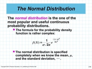
Education, Inc. publishing as Prentice Hall 2-66 The Normal Distribution The normal distribution is the one of the most popular and useful continuous probability distributions. The formula for the probability density function is rather complex: 2 2 2 2 1 ) ( ) ( x e X f The normal distribution is specified completely when we know the mean, µ, and the standard deviation, .
67.
Copyright ©2012 Pearson
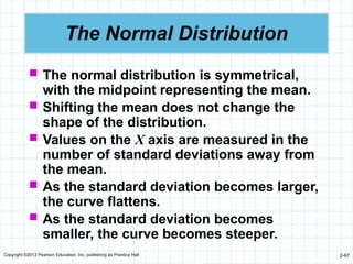
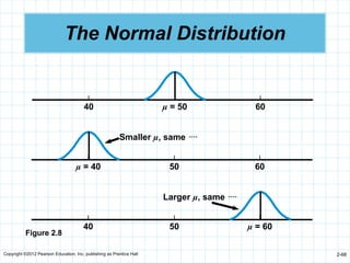
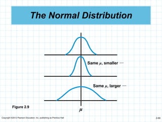
Education, Inc. publishing as Prentice Hall 2-67 The Normal Distribution The normal distribution is symmetrical, with the midpoint representing the mean. Shifting the mean does not change the shape of the distribution. Values on the X axis are measured in the number of standard deviations away from the mean. As the standard deviation becomes larger, the curve flattens. As the standard deviation becomes smaller, the curve becomes steeper.
68.
Copyright ©2012 Pearson
Education, Inc. publishing as Prentice Hall 2-68 The Normal Distribution | | | 40 µ = 50 60 | | | µ = 40 50 60 Smaller µ, same | | | 40 50 µ = 60 Larger µ, same Figure 2.8
69.
Copyright ©2012 Pearson
Education, Inc. publishing as Prentice Hall 2-69 µ The Normal Distribution Figure 2.9 Same µ, smaller Same µ, larger
70.
Copyright ©2012 Pearson
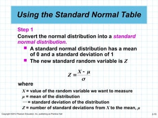
Education, Inc. publishing as Prentice Hall 2-70 Using the Standard Normal Table Step 1 Convert the normal distribution into a standard normal distribution. A standard normal distribution has a mean of 0 and a standard deviation of 1 The new standard random variable is Z X Z where X = value of the random variable we want to measure µ = mean of the distribution = standard deviation of the distribution Z = number of standard deviations from X to the mean, µ
71.
Copyright ©2012 Pearson
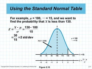
Education, Inc. publishing as Prentice Hall 2-71 Using the Standard Normal Table For example, µ = 100, = 15, and we want to find the probability that X is less than 130. 15 100 130 X Z dev std 2 15 30 | | | | | | | 55 70 85 100 115 130 145 | | | | | | | –3 –2 –1 0 1 2 3 X = IQ X Z µ = 100 = 15 P(X < 130) Figure 2.10
72.
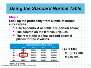
Copyright ©2012 Pearson
Education, Inc. publishing as Prentice Hall 2-72 Using the Standard Normal Table Step 2 Look up the probability from a table of normal curve areas. Use Appendix A or Table 2.9 (portion below). The column on the left has Z values. The row at the top has second decimal places for the Z values. AREA UNDER THE NORMAL CURVE Z 0.00 0.01 0.02 0.03 1.8 0.96407 0.96485 0.96562 0.96638 1.9 0.97128 0.97193 0.97257 0.97320 2.0 0.97725 0.97784 0.97831 0.97882 2.1 0.98214 0.98257 0.98300 0.98341 2.2 0.98610 0.98645 0.98679 0.98713 Table 2.9 (partial) P(X < 130) = P(Z < 2.00) = 0.97725
73.
Copyright ©2012 Pearson
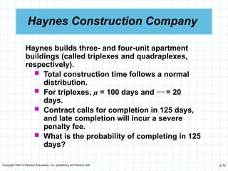
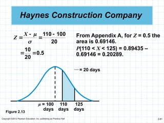
Education, Inc. publishing as Prentice Hall 2-73 Haynes Construction Company Haynes builds three- and four-unit apartment buildings (called triplexes and quadraplexes, respectively). Total construction time follows a normal distribution. For triplexes, µ = 100 days and = 20 days. Contract calls for completion in 125 days, and late completion will incur a severe penalty fee. What is the probability of completing in 125 days?
74.
Copyright ©2012 Pearson
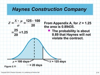
Education, Inc. publishing as Prentice Hall 2-74 Haynes Construction Company From Appendix A, for Z = 1.25 the area is 0.89435. The probability is about 0.89 that Haynes will not violate the contract. 20 100 125 X Z 25 1 20 25 . µ = 100 days X = 125 days = 20 days Figure 2.11
75.
Copyright ©2012 Pearson
Education, Inc. publishing as Prentice Hall 2-75 Haynes Construction Company Suppose that completion of a triplex in 75 days or less will earn a bonus of $5,000. What is the probability that Haynes will get the bonus?
76.
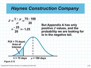
Copyright ©2012 Pearson
Education, Inc. publishing as Prentice Hall 2-76 Haynes Construction Company But Appendix A has only positive Z values, and the probability we are looking for is in the negative tail. 20 100 75 X Z 25 1 20 25 . Figure 2.12 µ = 100 days X = 75 days P(X < 75 days) Area of Interest
77.
Copyright ©2012 Pearson
Education, Inc. publishing as Prentice Hall 2-77 Haynes Construction Company Because the curve is symmetrical, we can look at the probability in the positive tail for the same distance away from the mean. 20 100 75 X Z 25 1 20 25 . µ = 100 days X = 125 days P(X > 125 days) Area of Interest
78.
Copyright ©2012 Pearson
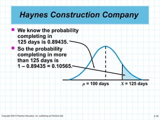
Education, Inc. publishing as Prentice Hall 2-78 Haynes Construction Company µ = 100 days X = 125 days We know the probability completing in 125 days is 0.89435. So the probability completing in more than 125 days is 1 – 0.89435 = 0.10565.
79.
Copyright ©2012 Pearson
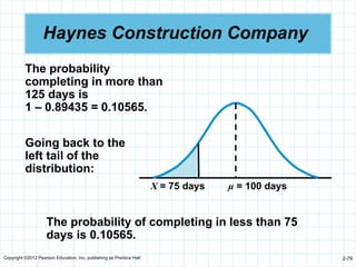
Education, Inc. publishing as Prentice Hall 2-79 Haynes Construction Company µ = 100 days X = 75 days The probability of completing in less than 75 days is 0.10565. Going back to the left tail of the distribution: The probability completing in more than 125 days is 1 – 0.89435 = 0.10565.
80.
Copyright ©2012 Pearson
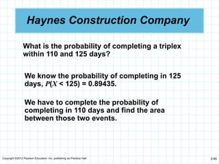
Education, Inc. publishing as Prentice Hall 2-80 Haynes Construction Company What is the probability of completing a triplex within 110 and 125 days? We know the probability of completing in 125 days, P(X < 125) = 0.89435. We have to complete the probability of completing in 110 days and find the area between those two events.
81.
Copyright ©2012 Pearson
Education, Inc. publishing as Prentice Hall 2-81 Haynes Construction Company From Appendix A, for Z = 0.5 the area is 0.69146. P(110 < X < 125) = 0.89435 – 0.69146 = 0.20289. 20 100 110 X Z 5 0 20 10 . Figure 2.13 µ = 100 days 125 days = 20 days 110 days
82.
Copyright ©2012 Pearson
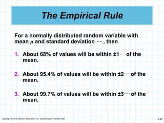
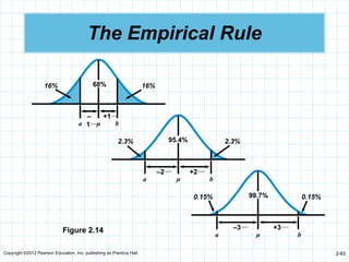
Education, Inc. publishing as Prentice Hall 2-82 The Empirical Rule For a normally distributed random variable with mean µ and standard deviation , then 1. About 68% of values will be within ±1 of the mean. 2. About 95.4% of values will be within ±2 of the mean. 3. About 99.7% of values will be within ±3 of the mean.
83.
Copyright ©2012 Pearson
Education, Inc. publishing as Prentice Hall 2-83 The Empirical Rule Figure 2.14 68% 16% 16% – 1 +1 a µ b 95.4% 2.3% 2.3% –2 +2 a µ b 99.7% 0.15% 0.15% –3 +3 a µ b
84.
Copyright ©2012 Pearson
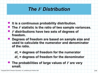
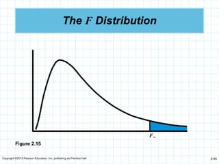
Education, Inc. publishing as Prentice Hall 2-84 The F Distribution It is a continuous probability distribution. The F statistic is the ratio of two sample variances. F distributions have two sets of degrees of freedom. Degrees of freedom are based on sample size and used to calculate the numerator and denominator of the ratio. The probabilities of large values of F are very small. df1 = degrees of freedom for the numerator df2 = degrees of freedom for the denominator
85.
Copyright ©2012 Pearson
Education, Inc. publishing as Prentice Hall 2-85 F The F Distribution Figure 2.15
86.
Copyright ©2012 Pearson
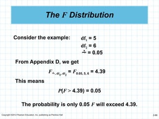
Education, Inc. publishing as Prentice Hall 2-86 The F Distribution df1 = 5 df2 = 6 = 0.05 Consider the example: From Appendix D, we get F, df1, df2 = F0.05, 5, 6 = 4.39 This means P(F > 4.39) = 0.05 The probability is only 0.05 F will exceed 4.39.
87.
Copyright ©2012 Pearson
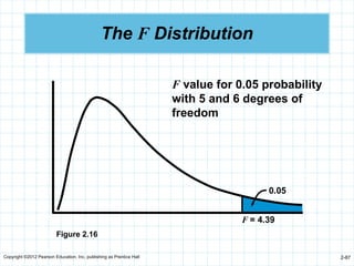
Education, Inc. publishing as Prentice Hall 2-87 The F Distribution Figure 2.16 F = 4.39 0.05 F value for 0.05 probability with 5 and 6 degrees of freedom
88.
Copyright ©2012 Pearson
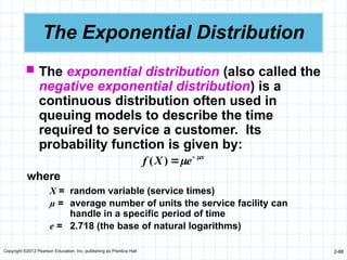
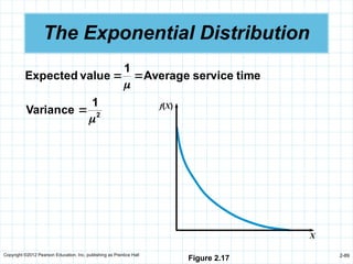
Education, Inc. publishing as Prentice Hall 2-88 The Exponential Distribution The exponential distribution (also called the negative exponential distribution) is a continuous distribution often used in queuing models to describe the time required to service a customer. Its probability function is given by: x e X f ) ( where X = random variable (service times) µ = average number of units the service facility can handle in a specific period of time e = 2.718 (the base of natural logarithms)
89.
Copyright ©2012 Pearson
Education, Inc. publishing as Prentice Hall 2-89 The Exponential Distribution time service Average 1 value Expected 2 1 Variance f(X) X Figure 2.17
90.
Copyright ©2012 Pearson
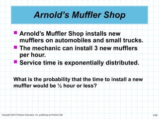
Education, Inc. publishing as Prentice Hall 2-90 Arnold’s Muffler Shop Arnold’s Muffler Shop installs new mufflers on automobiles and small trucks. The mechanic can install 3 new mufflers per hour. Service time is exponentially distributed. What is the probability that the time to install a new muffler would be ½ hour or less?
91.
Copyright ©2012 Pearson
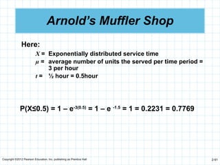
Education, Inc. publishing as Prentice Hall 2-91 Arnold’s Muffler Shop Here: X = Exponentially distributed service time µ = average number of units the served per time period = 3 per hour t = ½ hour = 0.5hour P(X≤0.5) = 1 – e-3(0.5) = 1 – e -1.5 = 1 = 0.2231 = 0.7769
92.
Copyright ©2012 Pearson
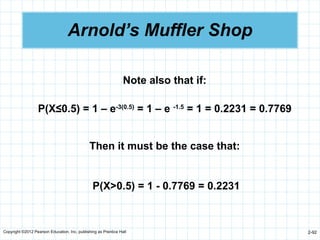
Education, Inc. publishing as Prentice Hall 2-92 Arnold’s Muffler Shop P(X≤0.5) = 1 – e-3(0.5) = 1 – e -1.5 = 1 = 0.2231 = 0.7769 Note also that if: Then it must be the case that: P(X>0.5) = 1 - 0.7769 = 0.2231
93.
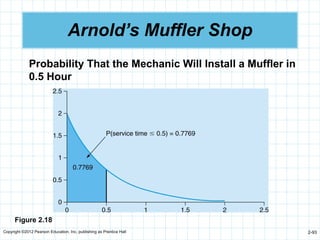
Copyright ©2012 Pearson
Education, Inc. publishing as Prentice Hall 2-93 Arnold’s Muffler Shop Probability That the Mechanic Will Install a Muffler in 0.5 Hour Figure 2.18
94.
Copyright ©2012 Pearson
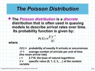
Education, Inc. publishing as Prentice Hall 2-94 The Poisson Distribution The Poisson distribution is a discrete distribution that is often used in queuing models to describe arrival rates over time. Its probability function is given by: ! ) ( X e X P x where P(X) = probability of exactly X arrivals or occurrences = average number of arrivals per unit of time (the mean arrival rate) e = 2.718, the base of natural logarithms X = specific value (0, 1, 2, 3, …) of the random variable
95.
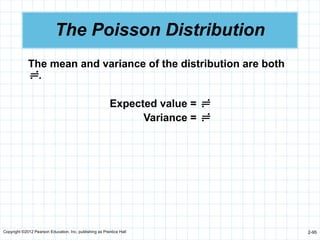
Copyright ©2012 Pearson
Education, Inc. publishing as Prentice Hall 2-95 The Poisson Distribution The mean and variance of the distribution are both . Expected value = Variance =
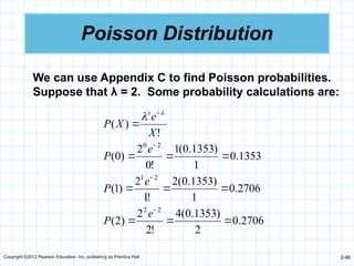
96.
Copyright ©2012 Pearson
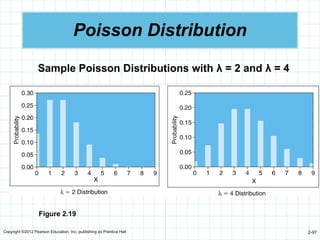
Education, Inc. publishing as Prentice Hall 2-96 Poisson Distribution We can use Appendix C to find Poisson probabilities. Suppose that λ = 2. Some probability calculations are: 2706 . 0 2 ) 1353 . 0 ( 4 ! 2 2 ) 2 ( 2706 . 0 1 ) 1353 . 0 ( 2 ! 1 2 ) 1 ( 1353 . 0 1 ) 1353 . 0 ( 1 ! 0 2 ) 0 ( ! ) ( 2 2 2 1 2 0 e P e P e P X e X P x
97.
Copyright ©2012 Pearson
Education, Inc. publishing as Prentice Hall 2-97 Poisson Distribution Figure 2.19 Sample Poisson Distributions with λ = 2 and λ = 4
98.
Copyright ©2012 Pearson
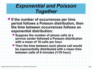
Education, Inc. publishing as Prentice Hall 2-98 Exponential and Poisson Together If the number of occurrences per time period follows a Poisson distribution, then the time between occurrences follows an exponential distribution: Suppose the number of phone calls at a service center followed a Poisson distribution with a mean of 10 calls per hour. Then the time between each phone call would be exponentially distributed with a mean time between calls of 6 minutes (1/10 hour).
99.
Copyright ©2012 Pearson
Education, Inc. publishing as Prentice Hall 2-99 Copyright All rights reserved. No part of this publication may be reproduced, stored in a retrieval system, or transmitted, in any form or by any means, electronic, mechanical, photocopying, recording, or otherwise, without the prior written permission of the publisher. Printed in the United States of America.
Download
![Copyright ©2012 Pearson Education, Inc. publishing as Prentice Hall 2-50
Variance of a
Discrete Probability Distribution
For a discrete probability distribution the
variance can be computed by
)
(
)]
(
[
n
i
i
i X
P
X
E
X
1
2
2
Variance
σ
where
i
X
)
(X
E
)
( i
X
P
= random variable’s possible values
= expected value of the random variable
= difference between each value of the random
variable and the expected mean
= probability of each possible value of the
random variable
)]
(
[ X
E
Xi ](https://image.slidesharecdn.com/ch02probabilityconceptsandapplications-250318105729-2766e8fd/85/Ch02-Probability-Concepts-and-Applications-pptx-50-320.jpg)
![Copyright ©2012 Pearson Education, Inc. publishing as Prentice Hall 2-51
Variance of a
Discrete Probability Distribution
For Dr. Shannon’s class:
)
(
)]
(
[
variance
5
1
2
i
i
i X
P
X
E
X
)
.
(
)
.
(
)
.
(
)
.
(
variance 2
0
9
2
4
1
0
9
2
5 2
2
)
.
(
)
.
(
)
.
(
)
.
( 3
0
9
2
2
3
0
9
2
3 2
2
)
.
(
)
.
( 1
0
9
2
1 2
29
1
361
0
243
0
003
0
242
0
441
0
.
.
.
.
.
.
](https://image.slidesharecdn.com/ch02probabilityconceptsandapplications-250318105729-2766e8fd/85/Ch02-Probability-Concepts-and-Applications-pptx-51-320.jpg)